
Estimating the Renovation Cost of Water, Sewage, and Gas Pipeline Networks: Multiple Regression Analysis to the Appraisal of a Reliable Cost Estimator for Urban Regeneration Works


Abstract
:1. Introduction
- What are the minimum explanatory variables needed to make a sufficiently accurate estimate of urban regeneration costs involving multiple infrastructure networks simultaneously?
- Does it make sense to differentiate cost functions according to the different urban contexts of historical centres and peripheral areas, and what factors eventually influence this differentiation?
- Build a unique cost function for those urban restructuring interventions that involve several types of infrastructure (roads and masonries; sewer, water, and gas networks);
- Establish whether it is necessary to differentiate cost functions according to the urban context, adopting different functions for historical centres and peripheral areas;
- Determine, by testing various models (linear, linear-logarithmic, logarithmic-linear, and exponential), the one that returns a more accurate estimate of costs;
- Identify the minimum number of explanatory variables that can explain the model;
- Implement the case studies conducted in Italy about the application of the MRA to estimate the renovation costs of sewer, water, and gas infrastructures [17]. This objective is interesting if contextualised concerning the not always easy execution of the works in Italian historical centres (and in those countries characterised by similar urban structures).
2. Literature Analysis
3. Methods
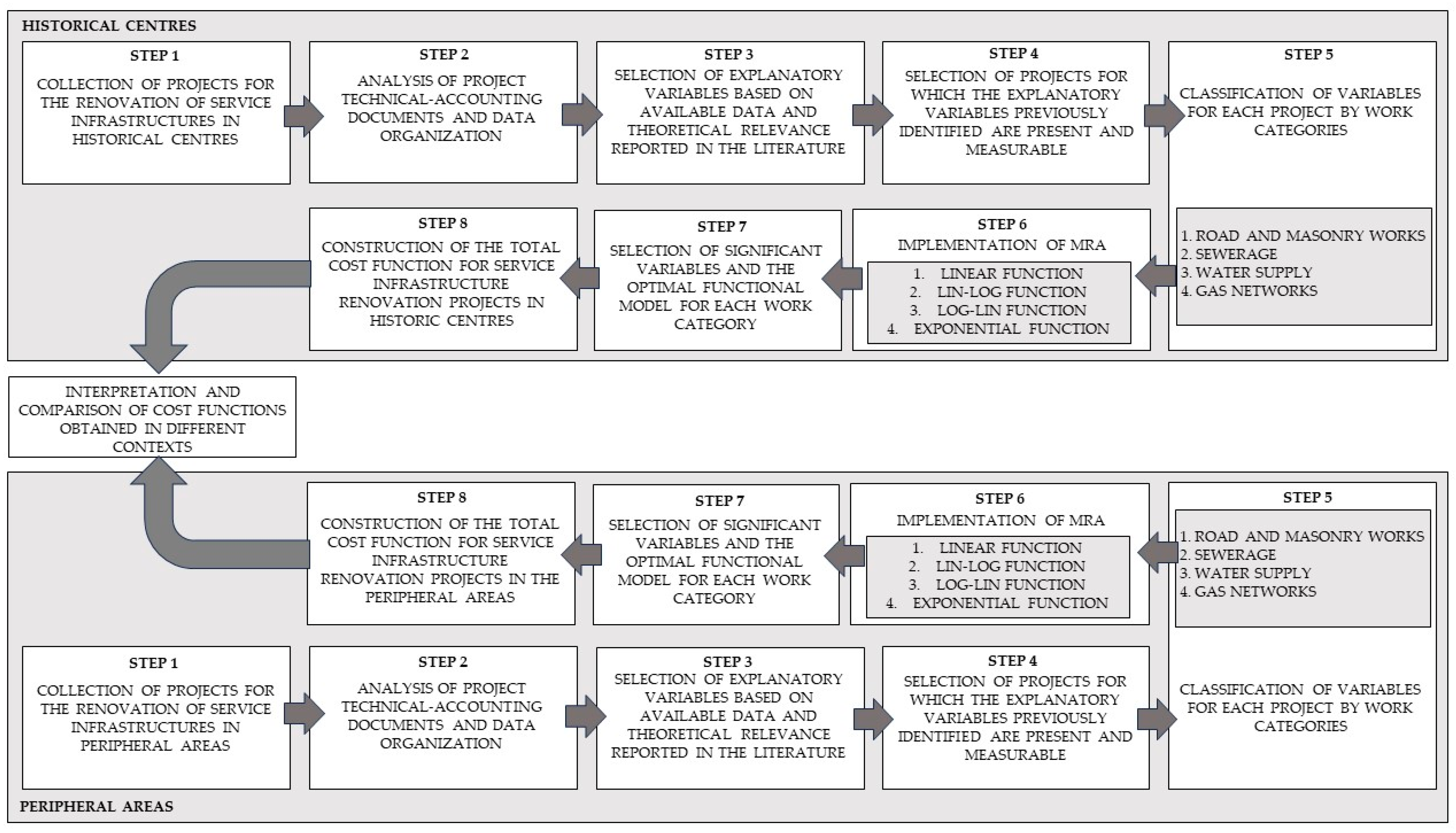
3.1. Steps of this Study
3.1.1. Step 1: Collection of Projects for the Renovation of Service Infrastructures
3.1.2. Step 2: Analysis of Project Technical-Accounting Documents and Data Organization
3.1.3. Step 3: Selection of Explanatory Variables Based on Available Data and Theoretical Relevance Reported in the Literature
3.1.4. Step 4: Selection of Projects for Which the Explanatory Variables Previously Identified Are Present and Measurable
3.1.5. Step 5: Classification of Variables for Each Project by Work Categories
3.1.6. Step 6: Implementation of Multiple Regression Analysis
3.1.7. Step 7: Selection of Significant Variables and the Optimal Functional Model for Each Work Category
3.1.8. Step 8: Construction of the Total Cost Function
3.2. The Variables That Influence the Renovation Cost
- L = length of the networks built (expressed in linear meters);
- S = renewed pavement surface (expressed in square meters);
- E = difficulty in the execution of the work (measured in dimensionless units);
- W = average width of the road section for intervention sites (expressed in linear meters);
- D = average diameter of the pipelines weighed on the length of the sections made and corrected with numerical coefficients proportional to the different costs of the materials used (expressed in millimetres);
- P = number of special pieces per pipeline linear metre (measured in dimensionless units).
3.2.1. Variables That Influence the Cost of Road and Masonry Works
- = average width of the road for the jth intervention;
- = width of the road for the ith section of the jth intervention;
- = length of the ith section of the jth intervention;
- = total length of the jth intervention.
3.2.2. Variables That Influence the Cost of Sewerage Water Supply and Gas Networks
- = average diameter of the pipeline of the jth intervention;
- = diameter of the ith segment of the pipeline of the jth intervention;
- = length of the ith segment of the jth intervention;
- = total length of the jth intervention.
- 1.8 for ductile iron pipes inserted in a reinforced concrete tunnel;
- 1.6 for synthetic resin pipes inserted in a reinforced concrete tunnel;
- 1.3 for ductile iron pipes;
- 1.25 for steel pipes;
- 1.2 for concrete pipes turbovibrocompressed;
- 1 for rigid PVC pipes;
- 1 for polyethylene pipes.
3.3. The Total Cost Function
- = total cost of the four categories of work;
- = cost of road and masonry works;
- = cost of renovation of the sewer network;
- = cost of renovation of the water network;
- = cost of renovation of the gas network.
4. Results
4.1. Application and Results in the Case of Interventions in Historical Centres
4.1.1. Road and Masonry Works
4.1.2. Sewerage
4.1.3. Water Supply
4.1.4. Gas Network
4.2. Application and Results in the Case of Interventions in Peripheral Areas
4.2.1. Road and Masonry Works
4.2.2. Sewerage
4.2.3. Water Supply
4.2.4. Gas Network
4.3. The Total Cost Function
5. Discussion
5.1. Historical Centres
5.2. Peripheral Areas
5.3. Implications of the Research
5.4. Limitations of Research and Future Prospects
6. Conclusions
Author Contributions
Funding
Data Availability Statement
Conflicts of Interest
Appendix A

| Cases | Road and Masonry Works | Sewerage | Water Supply | Gas Network | |||||||||||||||||||
|---|---|---|---|---|---|---|---|---|---|---|---|---|---|---|---|---|---|---|---|---|---|---|---|
| Costs (MEUR) | L (m) | S (m2) | E | W (m) | Costs (MEUR) | L (m) | D (mm) | W (m) | E | P | Costs (MEUR) | L (m) | D (mm) | W (m) | E | P | Costs (MEUR) | L (m) | D (mm) | W (m) | E | P | |
| 1 | 0.388 | 2143 | 4217 | 3 | 4.5 | 0.081 | 380 | 400 | 4.5 | 3 | 0.02 | 0.147 | 1363 | 162.13 | 4.5 | 3 | 0.02 | 0.041 | 400 | 110 | 4.5 | 3 | 0.02 |
| 2 | 0.405 | 3093 | 3740 | 7.7 | 3.5 | 0.263 | 944 | 400 | 3.5 | 7.7 | 0.05 | 0.165 | 1144 | 138.81 | 3.5 | 7.7 | 0.05 | 0.071 | 1005 | 78.84 | 3.5 | 7.7 | 0.05 |
| 3 | 0.461 | 2422 | 3849 | 7.7 | 3.5 | 0.187 | 649 | 400 | 3.5 | 7.7 | 0.05 | 0.143 | 996 | 135.23 | 3.5 | 7.7 | 0.05 | 0.058 | 777 | 86.94 | 3.5 | 7.7 | 0.05 |
| 4 | 3.321 | 14,307 | 23,164 | 4.7 | 4 | 1.097 | 4094 | 423.01 | 4 | 4.7 | 0.04 | 0.636 | 5550 | 136.68 | 4 | 4.7 | 0.04 | 0.325 | 4663 | 95.98 | 4 | 4.7 | 0.04 |
| 5 | 0.411 | 1782 | 4663 | 4.7 | 5 | 0.062 | 797 | 243.41 | 5 | 4.7 | 0.01 | 0.032 | 437 | 115.06 | 5 | 4.7 | 0.01 | 0.063 | 548 | 297.73 | 5 | 4.7 | 0.01 |
| 6 | 0.690 | 5572 | 6439 | 4.7 | 5 | 0.263 | 2831 | 224.24 | 5 | 4.7 | 0.02 | 0.152 | 1552 | 115.1 | 5 | 4.7 | 0.02 | 0.162 | 1189 | 301.57 | 5 | 4.7 | 0.02 |
| 7 | 0.037 | 249 | 627 | 1 | 2.5 | 0.006 | 85 | 171.76 | 2.5 | 1 | 0.01 | 0.005 | 84 | 90 | 2.5 | 1 | 0.01 | 0.005 | 80 | 100 | 2.5 | 1 | 0.01 |
| 8 | 0.040 | 319 | 817 | 1 | 4 | 0.007 | 114 | 191.4 | 4 | 1 | 0.01 | 0.006 | 100 | 90 | 4 | 1 | 0.01 | 0.007 | 105 | 100 | 4 | 1 | 0.01 |
| 9 | 0.026 | 203 | 580 | 1 | 5 | 0.003 | 60 | 125 | 5 | 1 | 0.01 | 0.004 | 73 | 90 | 5 | 1 | 0.01 | 0.004 | 70 | 100 | 5 | 1 | 0.01 |
| 10 | 0.081 | 476 | 1240 | 3 | 3.5 | 0.013 | 160 | 202.81 | 3.5 | 3 | 0.01 | 0.009 | 156 | 90 | 3.5 | 3 | 0.01 | 0.011 | 160 | 100 | 3.5 | 3 | 0.01 |
| 11 | 0.447 | 1547 | 5565 | 3 | 15 | 0.096 | 670 | 420.46 | 15 | 3 | 0.02 | 0.032 | 250 | 158.6 | 15 | 3 | 0.02 | 0.100 | 627 | 165.37 | 15 | 3 | 0.02 |
| 12 | 0.063 | 621 | 1043 | 1 | 3.5 | 0.018 | 173 | 545.9 | 3.5 | 1 | 0.01 | 0.019 | 227 | 160 | 3.5 | 1 | 0.01 | 0.018 | 221 | 125 | 3.5 | 1 | 0.01 |
| 13 | 0.264 | 2624 | 4888 | 1 | 8 | 0.111 | 739 | 458.36 | 800 | 1 | 0.01 | 0.076 | 970 | 148.66 | 8 | 1 | 0.01 | 0.080 | 915 | 174.18 | 8 | 1 | 0.01 |
| 14 | 0.501 | 2815 | 15,800 | 1 | 15 | 0.149 | 1 | 465.37 | 15 | 1 | 0.01 | 0.084 | 750 | 244.4 | 15 | 1 | 0.01 | 0.124 | 835 | 321.89 | 15 | 1 | 0.01 |
| 15 | 0.140 | 1073 | 2500 | 1 | 8 | 0.040 | 675 | 258.82 | 8 | 1 | 0.01 | 0.029 | 202 | 260 | 8 | 1 | 0.01 | 0.017 | 196 | 125 | 8 | 1 | 0.01 |
| 16 | 0.116 | 963 | 1900 | 1 | 7 | 0.023 | 468 | 206.52 | 700 | 1 | 0.01 | 0.026 | 279 | 178.24 | 7 | 1 | 0.01 | 0.021 | 216 | 187.5 | 7 | 1 | 0.01 |
| 17 | 0.119 | 1190 | 1680 | 1 | 2.5 | 0.033 | 440 | 344.03 | 2.5 | 1 | 0.01 | 0.032 | 420 | 130 | 2.5 | 1 | 0.01 | 0.025 | 330 | 117.27 | 2.5 | 1 | 0.01 |
| 18 | 0.061 | 706 | 900 | 1 | 3 | 0.018 | 240 | 383.13 | 3 | 1 | 0.01 | 0.018 | 240 | 130 | 3 | 1 | 0.01 | 0.014 | 226 | 100 | 3 | 1 | 0.01 |
| 19 | 4.910 | 30,264 | 56,073 | 4.7 | 35 | 2.057 | 15,782 | 267.48 | 3.5 | 4.7 | 0.04 | 0.720 | 7965 | 169 | 3.5 | 4.7 | 0.04 | 0.544 | 6517 | 141.61 | 3.5 | 4.7 | 0.04 |
| Cases | Road and Masonry Works | Sewerage | Water Supply | Gas Network | ||||||||||||
|---|---|---|---|---|---|---|---|---|---|---|---|---|---|---|---|---|
| Cost Effective | Cost Expected | Residuals | Residuals Percentages | Cost Effective | Cost Expected | Residuals | Residuals Percentages | Cost Effective | Cost Expected | Residuals | Residuals Percentages | Cost Effective | Cost Expected | Residuals | Residuals Percentages | |
| 1 | 0.388 | 0.346 | 0.042 | 11% | 0.081 | 0.061 | 0.020 | 24% | 0.147 | 0.146 | 0.000 | 0% | 0.041 | 0.032 | 0.010 | 24% |
| 2 | 0.405 | 0.504 | −0.099 | −24% | 0.263 | 0.250 | 0.013 | 5% | 0.165 | 0.152 | 0.014 | 8% | 0.071 | 0.068 | 0.003 | 5% |
| 3 | 0.461 | 0.464 | −0.003 | −1% | 0.187 | 0.176 | 0.011 | 6% | 0.143 | 0.130 | 0.013 | 9% | 0.058 | 0.054 | 0.004 | 7% |
| 4 | 3.321 | 2.421 | 0.901 | 27% | 1.097 | 0.960 | 0.136 | 12% | 0.636 | 0.572 | 0.064 | 10% | 0.325 | 0.369 | −0.044 | −14% |
| 5 | 0.411 | 0.393 | 0.018 | 4% | 0.062 | 0.048 | 0.014 | 23% | 0.032 | 0.034 | −0.002 | −7% | 0.063 | 0.064 | −0.001 | −1% |
| 6 | 0.690 | 0.761 | −0.070 | −10% | 0.263 | 0.256 | 0.007 | 2% | 0.152 | 0.130 | 0.022 | 15% | 0.162 | 0.143 | 0.019 | 12% |
| 7 | 0.037 | 0.032 | 0.005 | 13% | 0.006 | 0.005 | 0.001 | 21% | 0.005 | 0.005 | 0.000 | 2% | 0.005 | 0.005 | 0.000 | −1% |
| 8 | 0.040 | 0.042 | −0.002 | −5% | 0.007 | 0.009 | −0.002 | −31% | 0.006 | 0.006 | 0.000 | −5% | 0.007 | 0.007 | 0.000 | 0% |
| 9 | 0.026 | 0.028 | −0.003 | −10% | 0.003 | 0.003 | 0.000 | 16% | 0.004 | 0.004 | 0.000 | −1% | 0.004 | 0.005 | −0.001 | −19% |
| 10 | 0.081 | 0.090 | −0.009 | −11% | 0.013 | 0.013 | 0.000 | −2% | 0.009 | 0.011 | −0.002 | −27% | 0.011 | 0.011 | 0.000 | −4% |
| 11 | 0.447 | 0.358 | 0.088 | 20% | 0.096 | 0.108 | −0.011 | −12% | 0.032 | 0.030 | 0.001 | 4% | 0.100 | 0.078 | 0.022 | 22% |
| 12 | 0.063 | 0.064 | −0.001 | −2% | 0.018 | 0.021 | −0.003 | −18% | 0.019 | 0.019 | 0.000 | 1% | 0.018 | 0.017 | 0.001 | 6% |
| 13 | 0.264 | 0.291 | −0.027 | −10% | 0.111 | 0.102 | 0.009 | 8% | 0.076 | 0.077 | 0.000 | −1% | 0.080 | 0.101 | −0.021 | −26% |
| 14 | 0.501 | 0.607 | −0.106 | −21% | 0.149 | 0.117 | 0.033 | 22% | 0.084 | 0.086 | −0.002 | −2% | 0.124 | 0.134 | −0.010 | −8% |
| 15 | 0.140 | 0.135 | 0.005 | 4% | 0.040 | 0.061 | −0.021 | −52% | 0.029 | 0.030 | −0.001 | −4% | 0.017 | 0.018 | −0.001 | −5% |
| 16 | 0.116 | 0.109 | 0.007 | 6% | 0.023 | 0.026 | −0.003 | −11% | 0.026 | 0.026 | 0.000 | 1% | 0.021 | 0.023 | −0.001 | −5% |
| 17 | 0.119 | 0.110 | 0.009 | 7% | 0.033 | 0.036 | −0.003 | −9% | 0.032 | 0.028 | 0.004 | 12% | 0.025 | 0.023 | 0.002 | 7% |
| 18 | 0.061 | 0.061 | 0.000 | −1% | 0.018 | 0.022 | −0.004 | −25% | 0.018 | 0.017 | 0.001 | 6% | 0.014 | 0.015 | −0.001 | −6% |
| 19 | 4.910 | 5.604 | −0.694 | −14% | 2.057 | 2.386 | −0.330 | −16% | 0.720 | 0.968 | −0.248 | −34% | 0.544 | 0.580 | −0.036 | −7% |
| Average | 0.657 | 0.654 | 0.003 | −1% | 0.238 | 0.245 | −0.007 | −2% | 0.123 | 0.130 | −0.007 | −1% | 0.089 | 0.092 | −0.003 | −1% |
Appendix B
| Cases | Road and Masonry Works | Sewerage | Water Supply | Gas Network | |||||||||||||||||||
|---|---|---|---|---|---|---|---|---|---|---|---|---|---|---|---|---|---|---|---|---|---|---|---|
| Costs (MEUR) | L (m) | S (m2) | E | W (m) | Costs (MEUR) | L (m) | D (mm) | W (m) | E | P | Costs (MEUR) | L (m) | D (mm) | W (m) | E | P | Costs (MEUR) | L (m) | D (mm) | W (m) | E | P | |
| 1 | 6.205 | 34,864 | 70,645 | 1 | 15 | 1.702 | 13,025 | 728 | 15 | 1 | 0.02 | 1.062 | 11,520 | 288 | 15 | 1 | 0.02 | 0.839 | 10,319 | 98 | 15 | 1 | 0.02 |
| 2 | 0.879 | 4965 | 10,324 | 1 | 8 | 0.284 | 1855 | 544 | 8 | 1 | 0.01 | 0.153 | 1650 | 252 | 8 | 1 | 0.01 | 0.122 | 1460 | 110 | 8 | 1 | 0.01 |
| 3 | 0.602 | 3830 | 8534 | 3 | 5 | 0.179 | 1431 | 546 | 5 | 3 | 0.01 | 0.116 | 1270 | 182 | 5 | 3 | 0.01 | 0.090 | 1129 | 100 | 5 | 3 | 0.01 |
| 4 | 2.359 | 13,245 | 30,121 | 1 | 15 | 0.693 | 4948 | 912 | 15 | 1 | 0.01 | 0.406 | 4470 | 252 | 15 | 1 | 0.01 | 0.340 | 3827 | 100 | 15 | 1 | 0.01 |
| 5 | 0.660 | 3421 | 5310 | 1 | 7 | 0.204 | 1278 | 408 | 7 | 1 | 0.01 | 0.146 | 1130 | 208 | 7 | 1 | 0.01 | 0.080 | 1013 | 100 | 7 | 1 | 0.01 |
| 6 | 0.876 | 5023 | 9534 | 1 | 8 | 0.305 | 1877 | 684 | 8 | 1 | 0.01 | 0.158 | 1655 | 221 | 8 | 1 | 0.01 | 0.121 | 1491 | 100 | 8 | 1 | 0.01 |
| 7 | 0.159 | 974 | 1921 | 4.7 | 4.5 | 0.021 | 363.89 | 455 | 4.5 | 4.7 | 0.01 | 0.023 | 320 | 140 | 4.5 | 4.7 | 0.01 | 0.030 | 290.1 | 108 | 4.5 | 4.7 | 0.01 |
| 8 | 2.549 | 14,232 | 29,136 | 1 | 15 | 0.664 | 5317 | 452 | 15 | 1 | 0.01 | 0.418 | 4720 | 306 | 15 | 1 | 0.01 | 0.341 | 4195 | 100 | 15 | 1 | 0.01 |
| 9 | 0.871 | 5023 | 10,943 | 3 | 7 | 0.250 | 1877 | 753 | 7 | 3 | 0.01 | 0.156 | 1645 | 182 | 7 | 3 | 0.01 | 0.179 | 1501 | 423 | 7 | 3 | 0.01 |
| 10 | 0.651 | 3954 | 8412 | 3 | 7 | 0.148 | 1477 | 340 | 7 | 3 | 0.01 | 0.125 | 1315 | 160 | 7 | 3 | 0.01 | 0.099 | 1162 | 101 | 7 | 3 | 0.01 |
| 11 | 1.009 | 5491 | 9986 | 1 | 15 | 0.417 | 2051 | 629 | 15 | 1 | 0.02 | 0.190 | 1784 | 221 | 15 | 1 | 0.02 | 0.180 | 1656 | 195 | 15 | 1 | 0.02 |
| 12 | 0.459 | 2965 | 6098 | 3 | 5 | 0.110 | 1108 | 283 | 5 | 3 | 0.01 | 0.088 | 965 | 176 | 5 | 3 | 0.01 | 0.070 | 892 | 108 | 5 | 3 | 0.01 |
| 13 | 0.509 | 3129 | 6012 | 1 | 8 | 0.220 | 1169 | 628 | 8 | 1 | 0.01 | 0.115 | 1130 | 104 | 8 | 1 | 0.01 | 0.080 | 830 | 86 | 8 | 1 | 0.01 |
| 14 | 8.549 | 48,656 | 80,121 | 1 | 8 | 2.405 | 18,178 | 397 | 8 | 1 | 0.04 | 1.499 | 16,120 | 389 | 8 | 1 | 0.04 | 1.120 | ##### | 100 | 8 | 1 | 0.04 |
| 15 | 5.660 | 32,054 | 55,012 | 1 | 8 | 1.653 | 11,975 | 618 | 8 | 1 | 0.02 | 0.966 | 10,632 | 317 | 8 | 1 | 0.02 | 0.749 | 9447 | 100 | 8 | 1 | 0.02 |
| 16 | 0.428 | 3021 | 6121 | 3 | 4.5 | 0.122 | 1129 | 570 | 4.5 | 3 | 0.01 | 0.093 | 1020 | 140 | 4.5 | 3 | 0.01 | 0.080 | 872 | 101 | 4.5 | 3 | 0.01 |
| 17 | 2.700 | 15,643 | 20,121 | 3 | 5 | 0.784 | 5844 | 298 | 5 | 3 | 0.02 | 0.487 | 5213 | 182 | 5 | 3 | 0.02 | 0.369 | 4586 | 136 | 5 | 3 | 0.02 |
| 18 | 0.940 | 5543 | 10,412 | 1 | 8 | 0.351 | 2071 | 794 | 8 | 1 | 0.01 | 0.163 | 1750 | 208 | 8 | 1 | 0.01 | 0.160 | 1722 | 90 | 8 | 1 | 0.01 |
| 19 | 0.809 | 4879 | 9812 | 1 | 7 | 0.298 | 1823 | 605 | 7 | 1 | 0.01 | 0.153 | 1576 | 229 | 7 | 1 | 0.01 | 0.121 | 1480 | 108 | 7 | 1 | 0.01 |
| 20 | 0.459 | 2987 | 6121 | 3 | 4.5 | 0.141 | 1116 | 524 | 4.5 | 3 | 0.01 | 0.091 | 992 | 170 | 4.5 | 3 | 0.01 | 0.080 | 879 | 100 | 4.5 | 3 | 0.01 |
| Cases | Road and Masonry Works | Sewerage | Water Supply | Gas Network | ||||||||||||
|---|---|---|---|---|---|---|---|---|---|---|---|---|---|---|---|---|
| Cost Effective | Cost Expected | Residuals | Residuals Percentages | Cost Effective | Cost Expected | Residuals | Residuals Percentages | Actual Cost | Cost Expected | Residuals | Residuals Percentages | Cost Effective | Cost Expected | Residuals | Residuals Percentages | |
| 1 | 6.205 | 6.195 | 0.010 | 0% | 1.702 | 1.718 | −0.016 | −1% | 1.062 | 1.050 | 0.012 | 1% | 0.839 | 0.832 | 0.007 | 1% |
| 2 | 0.879 | 0.854 | 0.025 | 3% | 0.284 | 0.288 | −0.004 | −1% | 0.153 | 0.161 | −0.008 | −5% | 0.122 | 0.128 | −0.006 | −5% |
| 3 | 0.602 | 0.625 | −0.023 | −4% | 0.179 | 0.184 | −0.005 | −3% | 0.116 | 0.117 | −0.001 | −1% | 0.090 | 0.093 | −0.003 | −3% |
| 4 | 2.359 | 2.380 | −0.021 | −1% | 0.693 | 0.703 | −0.010 | −1% | 0.406 | 0.409 | −0.003 | −1% | 0.340 | 0.329 | 0.011 | 3% |
| 5 | 0.660 | 0.572 | 0.088 | 13% | 0.204 | 0.202 | 0.002 | 1% | 0.146 | 0.115 | 0.031 | 21% | 0.080 | 0.089 | −0.010 | −12% |
| 6 | 0.876 | 0.864 | 0.012 | 1% | 0.305 | 0.308 | −0.003 | −1% | 0.158 | 0.161 | −0.003 | −2% | 0.121 | 0.129 | −0.008 | −7% |
| 7 | 0.159 | 0.117 | 0.043 | 27% | 0.021 | 0.000 | 0.021 | 100% | 0.023 | 0.025 | −0.002 | −9% | 0.030 | 0.028 | 0.002 | 8% |
| 8 | 2.549 | 2.555 | −0.005 | 0% | 0.664 | 0.689 | −0.024 | −4% | 0.418 | 0.431 | −0.012 | −3% | 0.341 | 0.358 | −0.017 | −5% |
| 9 | 0.871 | 0.855 | 0.017 | 2% | 0.250 | 0.264 | −0.014 | −6% | 0.156 | 0.150 | 0.006 | 4% | 0.179 | 0.179 | 0.000 | 0% |
| 10 | 0.651 | 0.666 | −0.015 | −2% | 0.148 | 0.163 | −0.016 | −11% | 0.125 | 0.121 | 0.004 | 3% | 0.099 | 0.101 | −0.002 | −2% |
| 11 | 1.009 | 1.012 | −0.003 | 0% | 0.417 | 0.398 | 0.019 | 4% | 0.190 | 0.195 | −0.005 | −3% | 0.180 | 0.177 | 0.003 | 2% |
| 12 | 0.459 | 0.473 | −0.013 | −3% | 0.110 | 0.112 | −0.002 | −2% | 0.088 | 0.090 | −0.003 | −3% | 0.070 | 0.076 | −0.005 | −8% |
| 13 | 0.509 | 0.530 | −0.021 | −4% | 0.220 | 0.217 | 0.004 | 2% | 0.115 | 0.115 | 0.000 | 0% | 0.080 | 0.076 | 0.004 | 5% |
| 14 | 8.549 | 8.563 | −0.014 | 0% | 2.405 | 2.441 | −0.036 | −1% | 1.499 | 1.499 | 0.000 | 0% | 1.120 | 1.126 | −0.006 | −1% |
| 15 | 5.660 | 5.633 | 0.026 | 0% | 1.653 | 1.579 | 0.074 | 4% | 0.966 | 0.972 | −0.007 | −1% | 0.749 | 0.746 | 0.004 | 0% |
| 16 | 0.428 | 0.478 | −0.049 | −12% | 0.122 | 0.151 | −0.029 | −24% | 0.093 | 0.095 | −0.002 | −2% | 0.080 | 0.072 | 0.008 | 10% |
| 17 | 2.700 | 2.710 | −0.009 | 0% | 0.784 | 0.754 | 0.030 | 4% | 0.487 | 0.486 | 0.001 | 0% | 0.369 | 0.367 | 0.003 | 1% |
| 18 | 0.940 | 0.956 | −0.015 | −2% | 0.351 | 0.346 | 0.005 | 1% | 0.163 | 0.170 | −0.006 | −4% | 0.160 | 0.145 | 0.014 | 9% |
| 19 | 0.809 | 0.829 | −0.020 | −2% | 0.298 | 0.292 | 0.007 | 2% | 0.153 | 0.154 | −0.001 | 0% | 0.121 | 0.127 | −0.006 | −5% |
| 20 | 0.459 | 0.472 | −0.013 | −3% | 0.141 | 0.144 | −0.003 | −2% | 0.091 | 0.093 | −0.001 | −1% | 0.080 | 0.072 | 0.008 | 9% |
| Average | 1.867 | 1.867 | 0.000 | 1% | 0.548 | 0.548 | 0.000 | 3% | 0.330 | 0.330 | 0.000 | 0% | 0.262 | 0.262 | 0.000 | 0% |
References
- Kaddoura, K.; Zayed, T. Criticality model to prioritize pipeline rehabilitation decisions. In Proceedings of the Pipelines 2018: Condition Assessment, Construction, and Rehabilitation, Toronto, ON, Canada, 15–18 July 2018. [Google Scholar] [CrossRef]
- Wang, J.; Ulibarri, N.; Scott, T.A.; Davis, S.J. Environmental justice, infrastructure provisioning, and environmental impact assessment: Evidence from the California Environmental Quality Act. Environ. Sci. Policy 2023, 146, 66–75. [Google Scholar] [CrossRef]
- Globa, S.B.; Vasiljev, E.P.; Berezovaya, V.V.; Zyablikov, D.V. Risks and Financial Barriers to the Implementation of Sustainable Infrastructure Investment Projects in the Housing Sector. In Smart Green Innovations in Industry 4.0 for Climate Change Risk Management, 1st ed.; Popkova, E.G., Ed.; Springer International Publishing: Cham, Switzerland, 2023; pp. 239–245. [Google Scholar] [CrossRef]
- Brouwer, R.; Sharmin, D.F.; Elliott, S.; Liu, J.; Khan, M.R. Costs and benefits of improving water and sanitation in slums and non-slum neighborhoods in Dhaka, a fast-growing mega-city. Ecol. Econ. 2023, 207, 107763. [Google Scholar] [CrossRef]
- VanDerslice, J. Drinking water infrastructure and environmental disparities: Evidence and methodological considerations. Am. J. Public Health 2011, 101, S109–S114. [Google Scholar] [CrossRef] [PubMed]
- Quaranta, E.; Fuchs, S.; Liefting, H.J.; Schellart, A.; Pistocchi, A. Costs and benefits of combined sewer overflow management strategies at the European scale. J. Environ. Manag. 2022, 318, 115629. [Google Scholar] [CrossRef]
- Iqbal, H.; Tesfamariam, S.; Haider, H.; Sadiq, R. Inspection and maintenance of oil & gas pipelines: A review of policies. Struct. Infrastruct. Eng. 2017, 13, 794–815. [Google Scholar] [CrossRef]
- Hunt, D.V.; Jefferson, I.; Rogers, C.D. Assessing the sustainability of underground space usage—A toolkit for testing possible urban futures. J. Mt. Sci. 2011, 8, 211–222. [Google Scholar] [CrossRef]
- Alyami, S.H.; Abd El Aal, A.K.; Alqahtany, A.; Aldossary, N.A.; Jamil, R.; Almohassen, A.; Alzenifeer, B.M.; Kamh, H.M.; Fenais, A.S.; Alsalem, A.H. Developing a Holistic Resilience Framework for Critical Infrastructure Networks of Buildings and Communities in Saudi Arabia. Buildings 2023, 13, 179. [Google Scholar] [CrossRef]
- Heinimann, H.R.; Hatfield, K. Infrastructure resilience assessment, management and governance–state and perspectives. In Resilience and Risk; Springer: Berlin/Heidelberg, Germany, 2017; pp. 147–187. [Google Scholar] [CrossRef]
- Pericault, Y.; Viklander, M.; Hedström, A. Modelling the long-term sustainability impacts of coordination policies for urban infrastructure rehabilitation. Water Res. 2023, 236, 119912. [Google Scholar] [CrossRef]
- Carra, M.; Caselli, B.; Rossetti, S.; Zazzi, M. Widespread Urban Regeneration of Existing Residential Areas in European Medium-Sized Cities—A Framework to Locate Redevelopment Interventions. Sustainability 2023, 15, 13162. [Google Scholar] [CrossRef]
- Najafi, M.; Kulandaivel, G. Pipeline condition prediction using neural network models. In Proceedings of the Pipelines 2005: Optimizing Pipeline Design, Operations, and Maintenance in Today’s Economy, Houston, TX, USA, 21–24 August 2005. [Google Scholar] [CrossRef]
- Chughtai, F.; Zayed, T. Infrastructure condition prediction models for sustainable sewer pipelines. J. Perform. Constr. Facil. 2008, 22, 333–341. [Google Scholar] [CrossRef]
- Marchionni, V.; Lopes, N.; Mamouros, L.; Covas, D. Modelling sewer systems costs with multiple linear regression. Water Resour. Manag. 2014, 28, 4415–4431. [Google Scholar] [CrossRef]
- Lowe, D.J.; Emsley, M.W.; Harding, A. Harding, Predicting construction cost using multiple regression techniques. J. Constr. Eng. Manag. 2006, 132, 750–758. [Google Scholar] [CrossRef]
- Macchiaroli, M.; Dolores, L.; Nicodemo, L.; De Mare, G. Energy Efficiency in the Management of the Integrated Water Service. A Case Study on the White Certificates Incentive System. In Computational Science and Its Applications—ICCSA 2021. ICCSA 2021; Lecture Notes in Computer Science; Gervasi, O., Murgante, B., Misra, S., Garau, C., Blečić, I., Taniar, D., Apduhan, B.O., Rocha, A.M.A.C., Tarantino, E., Torre, C.M., Eds.; Springer: Cham, Switzerland, 2021; Volume 12956, pp. 202–217. [Google Scholar] [CrossRef]
- De Mare, G. Riurbanizzazione dei centri storici. Un modello per la classificazione dei dati, la stima preventiva e la verifica della congruità dei costi. In La Selezione dei Progetti e il Controllo dei Costi Nella Riqualificazione Urbana e Territoriale; Stanghellini, S., Ed.; Alinea Editrice: Firenze, Italy, 2004; pp. 243–268. ISBN 88-8125-837-4. [Google Scholar]
- Kim, G.H.; An, S.H.; Kang, K.I. Comparison of construction cost estimating models based on regression analysis, neural networks, and case-based reasoning. Build. Environ. 2004, 39, 1235–1242. [Google Scholar] [CrossRef]
- Skitmore, R.M.; Ng, S.T. Forecast models for actual construction time and cost. Build. Environ. 2003, 38, 1075–1083. [Google Scholar] [CrossRef]
- Trost, S.M.; Oberlender, G.D. Predicting accuracy of early cost estimates using factor analysis and multivariate regression. J. Constr. Eng. Manag. 2003, 129, 198–204. [Google Scholar] [CrossRef]
- Tam, C.M.; Fang, C.F. Comparative cost analysis of using high-performance concrete in tall building construction by artificial neural networks. ACI Struct. J. 1999, 96, 927–936. [Google Scholar]
- De Mare, G.; Di Piazza, F. The role of public-private partnerships in school building projects: Critical elements in the Italian model for implementing project financing. In Computational Science and Its Applications—ICCSA 2015. ICCSA 2015; Lecture Notes in Computer Science; Springer: Cham, Switzerland, 2015; Volume 9156, pp. 624–634. [Google Scholar] [CrossRef]
- Kwok, T.Y.; Yeung, D.Y. Constructive algorithmics for structure learning in feedforward neural networks for regression problems. IEEE Trans. Neural Netw. 1997, 8, 630–645. [Google Scholar] [CrossRef] [PubMed]
- Chen, D.; Burrell, P. Case-based reasoning system and artificial neural networks: A review. Neural Comput. Appl. 2001, 10, 264–276. [Google Scholar] [CrossRef]
- Riesbeck, C.; Schank, R. Inside Case-Based Reasoning; Lawrence Erlbaum Associate Publishers: Hillsdale, NY, USA, 1989. [Google Scholar]
- Petruseva, S.; Zileska-Pancovska, V.; Žujo, V.; Brkan-Vejzović, A. Construction costs forecasting: Comparison of the accuracy of linear regression and support vector machine models. Teh. Vjesn. 2017, 24, 1431–1438. [Google Scholar] [CrossRef]
- Mahamid, I. Early cost estimating for road construction projects using multiple regression techniques. AJCEB 2011, 11, 87–101. [Google Scholar] [CrossRef]
- Matel, E.; Vahdatikhaki, F.; Hosseinyalamdary, S.; Evers, T.; Voordijk, H. An artificial neural network approach for cost estimation of engineering services. Int. J. Constr. Manag. 2022, 22, 1274–1287. [Google Scholar] [CrossRef]
- Günaydın, H.M.; Doğan, S.Z. A neural network approach for early cost estimation of structural systems of buildings. Int. J. Constr. Manag. 2004, 22, 595–602. [Google Scholar] [CrossRef]
- Kim, H.J.; Seo, Y.C.; Hyun, C.T. A hybrid conceptual cost estimating model for large building projects. Autom. Constr. 2012, 25, 72–81. [Google Scholar] [CrossRef]
- Mahamid, I.; Bruland, A. Preliminary cost estimating models for road construction activities. In Proceedings of the FIG Congress 2010—Facing the Challenges—Building the Capacity, Sydney, Australia, 11–16 April 2010; Available online: https://citeseerx.ist.psu.edu/viewdoc/download?doi=10.1.1.603.1945&rep=rep1&type=pdf (accessed on 2 February 2023).
- Han, S.H.; Kim, D.Y.; Kim, H. Two-staged Early Cost Estimation for Highway Construction Projects. In Proceedings of the 25th International Symposium on Automation and Robotics in Construction ISARC-2008, Vilnius, Lithuania, 26–29 June 2008; Available online: https://citeseerx.ist.psu.edu/viewdoc/download?doi=10.1.1.1068.2640&rep=rep1&type=pdf (accessed on 2 February 2023).
- Sodikov, J. Cost estimation of highway projects in developing countries: Artificial neural network approach. J. East. Asia Soc. Transp. Stud. 2005, 6, 1036–1047. [Google Scholar] [CrossRef]
- Bell, L.C.; Bozai, G.A. Preliminary cost estimating for highway construction projects. Trans. Am. Assoc. Cost Eng. AACE 1987, 6, 1-C6. [Google Scholar]
- Marchionni, V.; Cabral, M.; Amado, C.; Covas, D. Estimating water supply infrastructure cost using regression technique. J. Water Resour. Plan. Manag. 2016, 142, 04016003. [Google Scholar] [CrossRef]
- Kasaplı, K. Artificial Neural Networks Usage for Cost Estimating on the Water Supply Networks. Master’s Thesis, İstanbul Technical University, İstanbul, Turkey, 2014; pp. 75–80. [Google Scholar]
- Walski, T.M. Planning-level capital cost estimates for pumping. J. Water Resour. Plan. Manag. 2012, 138, 307–310. [Google Scholar] [CrossRef]
- Fuchs-Hanusch, D.; Kornberger, B.; Friedl, F.; Scheucher, R.; Kainz, H. Whole of life cost calculations for water supply pipes. Water Asset Manag. Int. 2012, 8, 19–24. [Google Scholar]
- Swamee, P.K.; Sharma, A.K. Design of Water Supply Pipe Networks; John Wiley & Sons: Hoboken, NJ, USA, 2008; pp. 79–95. [Google Scholar]
- Clark, R.M.; Sivaganesan, M.; Selvakumar, A.; Sethi, V. Cost models for water supply distribution systems. J. Water Resour. Plan. Manag. 2002, 128, 312–321. [Google Scholar] [CrossRef]
- Sueri, M.; Erdal, M. Early Estimation of Sewerage Line Costs with Regression Analysis. Gazi Univ. J. Sci. 2022, 35, 822–832. [Google Scholar] [CrossRef]
- Rui, Z.H.; Metz, P.A.; Reynolds, D.B.; Chen, G.; Zhou, X.Y. Historical pipeline construction cost analysis. Int. J. Oil Gas Coal Technol. 2011, 4, 244–263. [Google Scholar] [CrossRef]
- Rui, Z.H.; Metz, P.A.; Chen, G. An analysis of inaccuracy in pipeline construction cost estimation. Int. J. Oil Gas Coal Technol. 2012, 5, 29–46. [Google Scholar] [CrossRef]
- Kaiser, M.J.; Liu, M. Cost factors and statistical evaluation of gas transmission pipeline construction and compressor-station cost in the USA, 2014–2019. Int. J. Oil Gas Coal Technol. 2021, 26, 422–452. [Google Scholar] [CrossRef]
- El-Kholy, A.M.; Tahwia, A.M.; Elsayed, M.M. Prediction of simulated cost contingency for steel reinforcement in building projects: ANN versus regression-based models. Int. J. Constr. Manag. 2022, 22, 1675–1689. [Google Scholar] [CrossRef]
- Alshamrani, O.S. Construction cost prediction model for conventional and sustainable college buildings in North America. J. Taibah Univ. Sci. 2017, 11, 315–323. [Google Scholar] [CrossRef]
- Asadi, S.; Amiri, S.S.; Mottahedi, M. On the development of multi-linear regression analysis to assess energy consumption in the early stages of building design. Energy Build. 2014, 85, 246–255. [Google Scholar] [CrossRef]
- Cho, H.G.; Kim, K.G.; Kim, J.Y.; Kim, G.H. A comparison of construction cost estimation using multiple regression analysis and neural network in elementary school project. J. Korea Inst. Build. Constr. 2013, 13, 66–74. [Google Scholar] [CrossRef]
- Chan, S.L.; Park, M. Project cost estimation using principal component regression. Constr. Manag. Econ. 2005, 23, 295–304. [Google Scholar] [CrossRef]
- Nuti, C.; Rasulo, A.; Vanzi, I. Seismic safety of network structures and infrastructures. Struct. Infrastruct. Eng. 2010, 6, 95–110. [Google Scholar] [CrossRef]
- Al-Thani, S.M.; Furlan, R. An Integrated Design Strategy for the Urban Regeneration of West Bay, Business District of Doha (State of Qatar). Designs 2020, 4, 55. [Google Scholar] [CrossRef]
- UNI EN 545:2100; Ductile Iron Pipes, Fittings and Accessories and Their Assemblies for Water Pipes—Requirements and Test Methods. Ente Italiano di Normazione: Milano, Italy, 2010.
- UNI EN 10221; Plastic Piping Systems for Water Distribution, and for Drainage and Sewerage under Pressure—Polyethylene (PE). Ente Italiano di Normazione: Milano, Italy, 1997.
- UNI EN 10224:2006; Unalloyed Steel Pipes and Fittings for Conveying Water and Other Aqueous. Ente Italiano di Normazione: Milano, Italy, 2006.
- UNI EN ISO 1452:2010; Plastic Piping Systems for Water Supply and Underground and Above-Ground Pressure Sewers and Drains—Unplasticized Polyvinyl Chloride (PVC-U). Ente Italiano di Normazione: Milano, Italy, 2010.
- De Mare, G.; Granata, M.F.; Forte, F. Investing in sports facilities: The Italian situation toward an Olympic perspective confidence intervals for the financial analysis of pools. In Computational Science and Its Applications—ICCSA 2015. ICCSA 2015; Lecture Notes in Computer Science; Gervasi, O., Murgante, B., Misra, S., Garau, C., Blečić, I., Taniar, D., Apduhan, B.O., Rocha, A.M.A.C., Tarantino, E., Torre, C.M., Eds.; Springer: Cham, Switzerland, 2015; Volume 9157, pp. 77–87. [Google Scholar] [CrossRef]
- Dolores, L.; Macchiaroli, M.; De Mare, G. Financial Impacts of the Energy Transition in Housing. Sustainability 2022, 14, 4876. [Google Scholar] [CrossRef]
- Macchiaroli, M.; Dolores, L.; De Mare, G.; Nicodemo, L. Tax Policies for Housing Energy Efficiency in Italy: A Risk Analysis Model for Energy Service Companies. Buildings 2023, 13, 582. [Google Scholar] [CrossRef]
- Liu, Y.; Shen, L.; Ren, Y.; Zhou, T. Regeneration towards suitability: A decision-making framework for determining urban regeneration mode and strategies. Habitat Int. 2023, 138, 102870. [Google Scholar] [CrossRef]
- Fasolino, I.; Grimaldi, M.; Zarra, T.; Naddeo, V. Implementation of Integrated Nuisances Action Plan. Chem. Eng. Trans. 2016, 54, 19–24. [Google Scholar] [CrossRef]
- Li, M.; Feng, X.; Han, Y.; Liu, X. Mobile augmented reality-based visualization framework for lifecycle O&M support of urban underground pipe networks. Tunn. Undergr. Space Technol. 2023, 136, 105069. [Google Scholar] [CrossRef]


| References | Infrastructure Type | Research Aim | Methods Used | Main Variables Used |
|---|---|---|---|---|
| Mahamid (2011) [28] | Road | To develop early cost-estimating models for road construction projects | MRA | Earthwork (cut, fill, and topping), base coarse pavement, curb stone, retaining wall concrete, sidewalk concrete, road marking, road length *, road width *. |
| Mahamid and Bruland (2010) [32] | Road | Estimation of the (total, per linear meter and per square meter) road construction cost | Linear MRA | Road length *, road width *, road surface thickness, road surface thickness after compaction, asphalt transport distance, and road surface area *. |
| Han et al. (2008) [33] | Road | Two-phase construction cost estimating model for schematic planning and preliminary design | CBA, RQB, CART and MRA models | Location, project type, contract type, construction period, total length of road *, road width *, total length of bridge, total length of tunnel. |
| Sodikov (2005) [34] | Road | To develop a more accurate estimating technique for highway projects | ANN and MRA | Predominant work activity, work duration, pavement width *, shoulder width, ground rise fall, average site clear/grub, earthwork volume, surface class category asphalt or concrete, base material. |
| Bell e Bozai (1987) [35] | Road | Estimation of long-term highway construction costs | MRA | Project length *, geographic zone, bid opening date, pay item number, material quantity, and pay item description. |
| Marchionni et al. (2016) [36] | Water | Definition and validation of reference cost functions for different types of water supply system assets | Linear MRA | Number of units, tank capacity, tank height, hydraulic power, pipe length *, trench width. Excavation depth, pipe material *, pipe diameter *. |
| Kasaplı (2014) [37] | Water | Estimation of the cost of construction of a potable water network comparing ANN and MRA | ANN and MRA | All available project data (physical and technological data). |
| Walski (2012) [38] | Water | Review of cost functions | Cost functions | Design type, design flow, design head, pumping power, flow rate, manometric head. |
| Fuchs-Hanusch et al. (2012) [39] | Water | Long-term cost estimation for maintenance and replacement of pipelines | Multivariate probabilistic model | Estimated years in which breaks occur (probability), pipe failure, water leaks, and road deterioration. |
| Swamee e Sharma (2008) [40] | Water | Determination of life cycle costs | Cost function | All available project data (physical and technological data). |
| Clark et al. (2002) [41] | Water | Presentation of equations that can be used to estimate the cost of building, expanding, rehabilitating, and repairing drinking water systems | Cost function | Type of activity, materials *, conditions (difficulty) of installation *, pipe diameter *, utility interference, traffic control. |
| Sueri ed Erdal (2022) [42] | Sewerage | To develop cost estimation models for sewerage networks | MRA | Pipe diameter *, line length *, excavation depth, manhole quantity, excavation quantity, backfill quantity, type *, shoring type, and excavation class. |
| Marchionni et al. (2014) [15] | Sewerage | Definition and validation of cost functions for various sewer system assets | MRA | Trench width, width of pavement removal and replacement *, depth above the top of the pipe, pipe diameter *, excavation depth, ratio of the length of pavement, and the total length of the pipes in the system. |
| Rui et al. (2011) [43] | Gas | To provide a reference for the cost of building the pipeline | cost analysis, cost function, learning curve | Pipeline diameter *, pipeline length *, pipeline capacity, year of completion, locations of pipelines. |
| Rui et al. (2012) [44] | Gas | To study the cost overruns of pipeline projects | MRA, statistical methods | Materials, labour, pipeline diameter, pipeline length, pipeline location, and year of completion. |
| Kaiser e Liu (2021) [45] | Gas | Estimation of pipeline construction costs | MRA, statistical methods | Route length * and line diameter *. |
| Cases | 1 | 2 | 3 | 4 | 5 | 6 | 7 | 8 | |||||||||||||||||||
| Sewerage | Lj | 380 | 944 | 649 | 4094 | 797 | 28 | 85 | 114 | ||||||||||||||||||
| Di,j | 250 | 250 | 250 | 250 | 400 | 500 | 600 | 200 | 250 | 315 | 400 | 500 | 200 | 250 | 315 | 400 | 500 | 160 | 200 | 160 | 200 | 250 | |||||
| Li,j | 380 | 944 | 649 | 3279 | 657 | 19 | 140 | 467 | 213 | 30 | 56 | 31 | 1654 | 756 | 108 | 201 | 112 | 60 | 25 | 62 | 22 | 30 | |||||
| Water supply | Lj | 1363 | 1144 | 996 | 5550 | 437 | 1552 | 84 | 100 | ||||||||||||||||||
| Di,j | 60 | 100 | 60 | 80 | 60 | 80 | 60 | 80 | 75 | 90 | 110 | 140 | 180 | 75 | 90 | 110 | 140 | 180 | 90 | 90 | |||||||
| Li,j | 338 | 1025 | 165 | 979 | 242 | 754 | 1129 | 4421 | 60 | 91 | 103 | 167 | 16 | 214 | 323 | 365 | 591 | 59 | 84 | 100 | |||||||
| Gas network | Lj | 400 | 1005 | 777 | 4663 | 548 | 1189 | 80 | 105 | ||||||||||||||||||
| Di,j | 110 | 63 | 110 | 63 | 110 | 63 | 90 | 110 | 114 | 168 | 273 | 323 | 88 | 114 | 168 | 273 | 323 | 406 | 80 | 80 | |||||||
| Li,j | 400 | 667 | 339 | 381 | 396 | 30 | 3199 | 1434 | 115 | 89 | 173 | 171 | 1 | 244 | 189 | 369 | 362 | 23 | 80 | 105 | |||||||
| Cases | 9 | 10 | 11 | 12 | 13 | 14 | |||||||||||||||||||||
| Sewerage | Lj | 60 | 160 | 670 | 173 | 739 | 1230 | ||||||||||||||||||||
| Di,j | 125 | 160 | 200 | 250 | 800 | 600 | 500 | 400 | 315 | 250 | 200 | 160 | 200 | 400 | 500 | 800 | 500 | 200 | 125 | 800 | 600 | 500 | 400 | 200 | |||
| Li,j | 60 | 75 | 40 | 45 | 120 | 60 | 100 | 63 | 37 | 165 | 40 | 85 | 8 | 54 | 111 | 99 | 263 | 326 | 51 | 15 | 300 | 300 | 60 | 555 | |||
| Water supply | Lj | 73 | 156 | 250 | 227 | 970 | 750 | ||||||||||||||||||||
| Di,j | 90 | 90 | 150 | 80 | 160 | 160 | 110 | 300 | 110 | ||||||||||||||||||
| Li,j | 73 | 156 | 150 | 100 | 227 | 750 | 220 | 360 | 390 | ||||||||||||||||||
| Gas network | Lj | 70 | 160 | 627 | 221 | 915 | 835 | ||||||||||||||||||||
| Di,j | 80 | 80 | 200 | 150 | 100 | 100 | 150 | 100 | 400 | 300 | 250 | 200 | 150 | ||||||||||||||
| Li,j | 70 | 160 | 340 | 275 | 12 | 221 | 720 | 195 | 190 | 210 | 15 | 20 | 400 | ||||||||||||||
| Cases | 15 | 16 | 17 | 18 | 19 | ||||||||||||||||||||||
| Sewerage | Lj | 675 | 468 | 440 | 240 | 15,782 | |||||||||||||||||||||
| Di,j | 500 | 400 | 315 | 250 | 200 | 125 | 110 | 600 | 315 | 250 | 200 | 160 | 125 | 110 | 500 | 400 | 315 | 500 | 400 | 315 | 600 | 500 | 400 | 315 | 250 | 200 | |
| Li,j | 100 | 99 | 36 | 59 | 66 | 151 | 65 | 43 | 17 | 33 | 72 | 186 | 11 | 105 | 47 | 48 | 345 | 70 | 40 | 130 | 70 | 535 | 835 | 3356 | 6470 | 4516 | |
| Water supply | Lj | 202 | 279 | 420 | 240 | 7965 | |||||||||||||||||||||
| Di,j | 200 | 150 | 100 | 100 | 100 | 60 | 200 | ||||||||||||||||||||
| Li,j | 202 | 207 | 72 | 420 | 240 | 3982 | 3983 | ||||||||||||||||||||
| Gas network | Lj | 196 | 216 | 330 | 226 | 6517 | |||||||||||||||||||||
| Di,j | 100 | 150 | 100 | 80 | 80 | 250 | 200 | 150 | 100 | 80 | |||||||||||||||||
| Li,j | 196 | 216 | 228 | 102 | 226 | 188 | 512 | 150 | 969 | 3360 | |||||||||||||||||
| Cases | 1 | 2 | 3 | 4 | 5 | 6 | 7 | 8 | ||||||||||||||||
| Sewerage | Lj | 13,025 | 1855 | 1431 | 4948 | 1278 | 1877 | 364 | 5317 | |||||||||||||||
| Di,j | 800 | 400 | 250 | 800 | 110 | 600 | 200 | 800 | 600 | 400 | 150 | 500 | 160 | 800 | 600 | 200 | 600 | 110 | 800 | 600 | 500 | 300 | 110 | |
| Li,j | 3256 | 5861 | 3908 | 618 | 1237 | 912 | 519 | 1649 | 2437 | 765 | 97 | 677 | 601 | 312 | 1268 | 297 | 256 | 108 | 45 | 790 | 830 | 923 | 2729 | |
| Water supply | Lj | 11,520 | 1650 | 1270 | 4470 | 1130 | 1655 | 320 | 4720 | |||||||||||||||
| Di,j | 300 | 150 | 80 | 300 | 90 | 200 | 110 | 300 | 140 | 80 | 60 | 300 | 110 | 300 | 150 | 75 | 140 | 300 | 150 | 60 | ||||
| Li,j | 2464 | 5421 | 3635 | 393 | 1257 | 423 | 847 | 1023 | 1212 | 754 | 1481 | 297 | 833 | 454 | 734 | 467 | 320 | 2046 | 312 | 2362 | ||||
| Gas network | Lj | 10,319 | 1460 | 1129 | 3827 | 1013 | 1491 | 290 | 4195 | |||||||||||||||
| Di,j | 110 | 100 | 80 | 110 | 80 | 100 | 80 | 80 | 63 | 110 | 100 | |||||||||||||
| Li,j | 2580 | 5159 | 2580 | 1460 | 1129 | 3827 | 1013 | 1491 | 145 | 145 | 4195 | |||||||||||||
| Cases | 9 | 10 | 11 | 12 | 13 | 14 | ||||||||||||||||||
| Sewerage | Lj | 1877 | 1477 | 2051 | 1108 | 1169 | 18,178 | |||||||||||||||||
| Di,j | 800 | 300 | 600 | 200 | 110 | 800 | 600 | 400 | 200 | 150 | 600 | 110 | 800 | 500 | 160 | 600 | 500 | 300 | 250 | 110 | ||||
| Li,j | 1229 | 647 | 595 | 533 | 349 | 673 | 612 | 110 | 543 | 114 | 391 | 717 | 532 | 608 | 29 | 121 | 809 | 6421 | 6543 | 4284 | ||||
| Water supply | Lj | 1645 | 1315 | 1784 | 965 | 1130 | 16,120 | |||||||||||||||||
| Di,j | 200 | 75 | 200 | 80 | 300 | 180 | 80 | 65 | 180 | 80 | 180 | 80 | 400 | 300 | 180 | 80 | 60 | |||||||
| Li,j | 855 | 790 | 877 | 438 | 509 | 543 | 352 | 380 | 926 | 39 | 271 | 859 | 2877 | 6121 | 421 | 932 | 5769 | |||||||
| Gas network | Lj | 1501 | 1162 | 1656 | 892 | 830 | 14,358 | |||||||||||||||||
| Di,j | 400 | 250 | 63 | 90 | 200 | 100 | 100 | 80 | 63 | 80 | 100 | |||||||||||||
| Li,j | 751 | 751 | 387 | 775 | 828 | 828 | 297 | 595 | 553 | 277 | 14,358 | |||||||||||||
| Cases | 15 | 16 | 17 | 18 | 19 | 20 | ||||||||||||||||||
| Sewerage | Lj | 11,975 | 1129 | 5844 | 2071 | 1823 | 1116 | |||||||||||||||||
| Di,j | 800 | 600 | 200 | 160 | 800 | 300 | 250 | 800 | 500 | 250 | 800 | 250 | 800 | 300 | 600 | 250 | 110 | |||||||
| Li,j | 1021 | 4479 | 2132 | 4344 | 637 | 215 | 277 | 173 | 2134 | 3537 | 1550 | 521 | 744 | 1078 | 882 | 212 | 22 | |||||||
| Water supply | Lj | 10,632 | 1020 | 5213 | 1750 | 1576 | 992 | |||||||||||||||||
| Di,j | 400 | 300 | 180 | 65 | 140 | 140 | 160 | 180 | 90 | 180 | 90 | |||||||||||||
| Li,j | 1695 | 2345 | 543 | 6049 | 1020 | 5213 | 1750 | 1509 | 67 | 882 | 110 | |||||||||||||
| Gas network | Lj | 9447 | 872 | 4586 | 1722 | 1480 | 879 | |||||||||||||||||
| Di,j | 100 | 63 | 80 | 100 | 200 | 100 | 80 | 90 | 63 | 100 | 80 | 80 | ||||||||||||
| Li,j | 9447 | 218 | 436 | 218 | 917 | 1834 | 917 | 574 | 1148 | 493 | 987 | 879 | ||||||||||||
| Cases | Sewerage | Water Supply | Gas Network | |||
|---|---|---|---|---|---|---|
| Pipeline Materials | Coefficients | Pipeline Materials | Coefficients | Pipeline Materials | Coefficients | |
| 1 | Synthetic resin in reinforced concrete tunnel | 1.6 | Ductile iron pipes inserted in a reinforced concrete tunnel | 1.8 | Polyethylene | 1 |
| 2 | Synthetic resin in reinforced concrete tunnel | 1.6 | Ductile iron pipes inserted in a reinforced concrete tunnel | 1.8 | Polyethylene | 1 |
| 3 | Synthetic resin in reinforced concrete tunnel | 1.6 | Ductile iron pipes inserted in a reinforced concrete tunnel | 1.8 | Polyethylene | 1 |
| 4 | Synthetic resin in reinforced concrete tunnel | 1.6 | Ductile iron pipes inserted in a reinforced concrete tunnel | 1.8 | Polyethylene | 1 |
| 5 | Rigid PVC | 1 | Polyethylene | 1 | Steel pipes | 1.25 |
| 6 | Rigid PVC | 1 | Polyethylene | 1 | Steel pipes | 1.25 |
| 7 | Rigid PVC | 1 | Polyethylene | 1 | Steel pipes | 1.25 |
| 8 | Rigid PVC | 1 | Polyethylene | 1 | Steel pipes | 1.25 |
| 9 | Rigid PVC | 1 | Polyethylene | 1 | Steel pipes | 1.25 |
| 10 | Rigid PVC | 1 | Polyethylene | 1 | Steel pipes | 1.25 |
| 11 | Rigid PVC | 1 | Ductile iron pipes | 1.3 | Steel pipes | 1.25 |
| 12 | Turbovibrocompressed concrete | 1.2 | Polyethylene | 1 | Steel pipes | 1.25 |
| 13 | Turbovibrocompressed concrete | 1.2 | Polyethylene | 1 | Steel pipes | 1.25 |
| 14 | Turbovibrocompressed concrete | 1.2 | Ductile iron pipes and polyethylene | 1.3 and 1 | Ductile iron pipes | 1.3 |
| 15 | Rigid PVC | 1 | Ductile iron pipes | 1.3 | Steel pipes | 1.25 |
| 16 | Rigid PVC | 1 | Ductile iron pipes | 1.3 | Steel pipes | 1.25 |
| 17 | Rigid PVC | 1 | Ductile iron pipes | 1.3 | Steel pipes | 1.25 |
| 18 | Rigid PVC | 1 | Ductile iron pipes | 1.3 | Steel pipes | 1.25 |
| 19 | Rigid PVC | 1 | Ductile iron pipes | 1.3 | Steel pipes | 1.25 |
| Cases | Sewerage | Water Supply | Gas Network | |||
|---|---|---|---|---|---|---|
| Pipeline Materials | Coefficients | Pipeline Materials | Coefficients | Pipeline Materials | Coefficients | |
| 1 | Synthetic resin in reinforced concrete tunnel | 1.6 | Ductile iron pipes inserted in a reinforced concrete tunnel | 1.8 | Polyethylene | 1 |
| 2 | Synthetic resin in reinforced concrete tunnel | 1.6 | Ductile iron pipes inserted in a reinforced concrete tunnel | 1.8 | Polyethylene | 1 |
| 3 | Turbovibrocompressed concrete | 1.2 | Ductile iron pipes | 1.3 | Steel pipes | 1.25 |
| 4 | Synthetic resin in reinforced concrete tunnel | 1.6 | Ductile iron pipes inserted in a reinforced concrete tunnel | 1.8 | Polyethylene | 1 |
| 5 | Turbovibrocompressed concrete | 1.2 | Ductile iron pipes | 1.3 | Steel pipes | 1.25 |
| 6 | Turbovibrocompressed concrete | 1.2 | Ductile iron pipes | 1.3 | Steel pipes | 1.25 |
| 7 | Rigid PVC | 1 | Polyethylene | 1 | Steel pipes | 1.25 |
| 8 | Synthetic resin in reinforced concrete tunnel | 1.6 | Ductile iron pipes inserted in a reinforced concrete tunnel | 1.8 | Polyethylene | 1 |
| 9 | Turbovibrocompressed concrete | 1.2 | Ductile iron pipes | 1.3 | Ductile iron pipes | 1.3 |
| 10 | Rigid PVC | 1 | Polyethylene | 1 | Steel pipes | 1.25 |
| 11 | Turbovibrocompressed concrete | 1.2 | Ductile iron pipes | 1.3 | Ductile iron pipes | 1.3 |
| 12 | Rigid PVC | 1 | Polyethylene | 1 | Steel pipes | 1.25 |
| 13 | Rigid PVC | 1 | Polyethylene | 1 | Steel pipes | 1.25 |
| 14 | Synthetic resin in reinforced concrete tunnel | 1.6 | Ductile iron pipes inserted in a reinforced concrete tunnel | 1.8 | Polyethylene | 1 |
| 15 | Synthetic resin in reinforced concrete tunnel | 1.6 | Ductile iron pipes inserted in a reinforced concrete tunnel | 1.8 | Polyethylene | 1 |
| 16 | Rigid PVC | 1 | Polyethylene | 1 | Steel pipes | 1.25 |
| 17 | Turbovibrocompressed concrete | 1.2 | Ductile iron pipes | 1.3 | Steel pipes | 1.25 |
| 18 | Turbovibrocompressed concrete | 1.2 | Ductile iron pipes | 1.3 | Steel pipes | 1.25 |
| 19 | Turbovibrocompressed concrete | 1.2 | Ductile iron pipes | 1.3 | Steel pipes | 1.25 |
| 20 | Rigid PVC | 1 | Polyethylene | 1 | Steel pipes | 1.25 |
| Cases | Historical Centres | Peripheral Areas | ||
|---|---|---|---|---|
| Total Network Angular Deviations | Total Network Angular Deviations | |||
| Measured P | Approximate P | Measured P | Approximate P | |
| 1 | 0.0166 | 0.015 | 0.0195 | 0.020 |
| 2 | 0.0448 | 0.045 | 0.0097 | 0.010 |
| 3 | 0.0473 | 0.045 | 0.0095 | 0.010 |
| 4 | 0.0407 | 0.040 | 0.0101 | 0.010 |
| 5 | 0.0072 | 0.005 | 0.0089 | 0.010 |
| 6 | 0.0158 | 0.015 | 0.0098 | 0.010 |
| 7 | 0.0000 | 0.005 | 0.0091 | 0.010 |
| 8 | 0.0087 | 0.010 | 0.0087 | 0.010 |
| 9 | 0.0000 | 0.005 | 0.0090 | 0.010 |
| 10 | 0.0093 | 0.010 | 0.0110 | 0.010 |
| 11 | 0.0150 | 0.015 | 0.0221 | 0.020 |
| 12 | 0.0030 | 0.005 | 0.0123 | 0.010 |
| 13 | 0.0093 | 0.010 | 0.0096 | 0.010 |
| 14 | 0.0000 | 0.005 | 0.0393 | 0.040 |
| 15 | 0.0121 | 0.010 | 0.0225 | 0.020 |
| 16 | 0.0000 | 0.005 | 0.0134 | 0.010 |
| 17 | 0.0024 | 0.005 | 0.0198 | 0.020 |
| 18 | 0.0066 | 0.005 | 0.0079 | 0.010 |
| 19 | 0.0432 | 0.040 | 0.0132 | 0.010 |
| 20 | - | - | 0.0088 | 0.010 |
| Regression Statistics | Linear | Lin-Log | Log-Lin | Exponential | Adjusted Exponential |
|---|---|---|---|---|---|
| Multiple R | 0.983 | 0.905 | 0.928 | 0.995 | 0.995 |
| R2 | 0.966 | 0.818 | 0.862 | 0.991 | 0.991 |
| Adjusted R2 | 0.957 | 0.766 | 0.823 | 0.988 | 0.989 |
| Standard error | 0.263 | 0.610 | 0.605 | 0.155 | 0.150 |
| Significance F | Linear | Lin-Log | Log-Lin | Exponential | Adjusted exponential |
| 0.000 | 0.000 | 0.000 | 0.000 | 0.000 | |
| Coefficients | Linear | Lin-Log | Log-Lin | Exponential | Adjusted exponential |
| Intercepts | −0.118 | −6.102 | −3.709 | −9.579 | −9.576 |
| W | 0.017 | −1.438 | 0.171 | −0.010 | Deleted |
| E | 0.011 | −0.288 | 0.278 | 0.314 | 0.316 |
| S | −0.000 | 1.584 | −0.000 | 0.613 | 0.604 |
| L | 0.000 | −0.482 | 0.000 | 0.400 | 0.408 |
| Standard error | Linear | Lin-Log | Log-Lin | Exponential | Adjusted exponential |
| Intercepts | 0.162 | 1.057 | 0.372 | 0.269 | 0.258 |
| W | 0.024 | 0.405 | 0.056 | 0.103 | Deleted |
| E | 0.031 | 0.237 | 0.071 | 0.060 | 0.057 |
| S | 0.000 | 0.537 | 0.000 | 0.137 | 0.095 |
| L | 0.000 | 0.498 | 0.000 | 0.127 | 0.097 |
| Significance of t | Linear | Lin-Log | Log-Lin | Exponential | Adjusted exponential |
| Intercepts | 0.478 | 0.000 | 0.000 | 0.000 | 0.000 |
| W | 0.507 | 0.003 | 0.009 | 0.923 | Deleted |
| E | 0.715 | 0.244 | 0.001 | 0.000 | 0.000 |
| S | 0.604 | 0.011 | 0.464 | 0.001 | 0.000 |
| L | 0.005 | 0.350 | 0.117 | 0.007 | 0.001 |
| Regression Statistics | Linear | Lin-Log | Log-Lin | Exponential | Adjusted Exponential |
|---|---|---|---|---|---|
| Multiple R | 0.982 | 0.893 | 0.931 | 0.995 | 0.993 |
| R2 | 0.964 | 0.797 | 0.867 | 0.990 | 0.987 |
| Adjusted R2 | 0.951 | 0.719 | 0.816 | 0.986 | 0.984 |
| Standard error | 0.112 | 0.268 | 0.741 | 0.201 | 0.216 |
| Significance F | Linear | Lin-Log | Log-Lin | Exponential | Adjusted exponential |
| 0.000 | 0.000 | 0.000 | 0.000 | 0.000 | |
| Coefficients | Linear | Lin-Log | Log-Lin | Exponential | Modified exponential |
| Intercepts | −0.0602 | 1.476 | −6.374 | −11.559 | −10.687 |
| L | 0.0001 | 0.327 | 0.000 | 0.908 | 0.930 |
| D | 0.0001 | −0.272 | 0.005 | 0.780 | 0.753 |
| W | −0.0030 | −0.271 | 0.102 | 0.040 | Deleted |
| D | −0.0373 | −0.247 | 0.329 | 0.210 | Deleted |
| P | 11.7543 | 0.252 | 6.577 | 0.368 | 0.510 |
| Standard error | Linear | Lin-Log | Log-Lin | Exponential | Adjusted exponential |
| Intercepts | 0.087 | 1.297 | 0.573 | 0.974 | 0.922 |
| L | 0.000 | 0.065 | 0.000 | 0.048 | 0.049 |
| D | 0.000 | 0.169 | 0.002 | 0.127 | 0.134 |
| W | 0.008 | 0.132 | 0.052 | 0.099 | Deleted |
| D | 0.024 | 0.135 | 0.156 | 0.102 | Deleted |
| P | 4.248 | 0.138 | 28.130 | 0.103 | 0.078 |
| Significance of t | Linear | Lin-Log | Log-Lin | Exponential | Adjusted exponential |
| Intercepts | 0.499 | 0.276 | 0.000 | 0.000 | 0.000 |
| L | 0.000 | 0.000 | 0.001 | 0.000 | 0.000 |
| D | 0.572 | 0.132 | 0.015 | 0.000 | 0.000 |
| W | 0.707 | 0.061 | 0.070 | 0.695 | Deleted |
| D | 0.137 | 0.091 | 0.054 | 0.059 | Deleted |
| P | 0.016 | 0.090 | 0.819 | 0.004 | 0.000 |
| Regression Statistics | Linear | Lin-Log | Log-Lin | Exponential | Adjusted Exponential |
|---|---|---|---|---|---|
| Multiple R | 0.993 | 0.892 | 0.920 | 0.997 | 0.997 |
| R2 | 0.987 | 0.796 | 0.846 | 0.994 | 0.994 |
| Adjusted R2 | 0.981 | 0.718 | 0.787 | 0.992 | 0.993 |
| Standard error | 0.028 | 0.108 | 0.701 | 0.133 | 0.128 |
| Significance F | Linear | Lin-Log | Log-Lin | Exponential | Adjusted exponential |
| 0.000 | 0.000 | 0.000 | 0.000 | 0.000 | |
| Coefficients | Linear | Lin-Log | Log-Lin | Exponential | Adjusted exponential |
| Intercepts | −0.0159 | 0.360 | −6.301 | −12.766 | −12.75 |
| L | 0.0001 | 0.134 | 0.000 | 0.915 | 0.92 |
| D | 0.0000 | −0.109 | 0.012 | 0.928 | 0.92 |
| W | 0.0006 | −0.025 | 0.009 | −0.004 | Deleted |
| D | −0.0028 | −0.090 | 0.360 | 0.174 | 0.17 |
| P | 2.2545 | 0.093 | −10.355 | 0.159 | 0.16 |
| Standard error | Linear | Lin-Log | Log-Lin | Exponential | Adjusted exponential |
| Intercepts | 0.025 | 0.630 | 0.621 | 0.773 | 0.67 |
| L | 0.000 | 0.033 | 0.000 | 0.040 | 0.04 |
| D | 0.000 | 0.127 | 0.005 | 0.155 | 0.12 |
| W | 0.002 | 0.063 | 0.059 | 0.078 | Deleted |
| D | 0.006 | 0.059 | 0.156 | 0.072 | 0.07 |
| P | 1.149 | 0.057 | 28.918 | 0.070 | 0.07 |
| Significance of t | Linear | Lin-Log | Log-Lin | Exponential | Adjusted exponential |
| Intercepts | 0.529 | 0.577 | 0.000 | 0.000 | 0.00 |
| L | 0.000 | 0.001 | 0.003 | 0.000 | 0.00 |
| D | 0.942 | 0.405 | 0.022 | 0.000 | 0.00 |
| W | 0.811 | 0.695 | 0.885 | 0.956 | Deleted |
| D | 0.661 | 0.150 | 0.039 | 0.031 | 0.05 |
| P | 0.071 | 0.128 | 0.726 | 0.042 | 0.03 |
| Regression Statistics | Linear | Lin-Log | Log-Lin | Exponential | Adjusted Exponential |
|---|---|---|---|---|---|
| Multiple R | 0.994 | 0.881 | 0.941 | 0.997 | 0.997 |
| R2 | 0.987 | 0.775 | 0.886 | 0.993 | 0.996 |
| Adjusted R2 | 0.982 | 0.689 | 0.842 | 0.991 | 0.991 |
| Standard error | 0.018 | 0.075 | 0.541 | 0.130 | 0.138 |
| Significance F | Linear | Lin-Log | Log-Lin | Exponential | Adjusted exponential |
| 0.000 | 0.000 | 0.000 | 0.000 | 0.000 | |
| Coefficients | Linear | Lin-Log | Log-Lin | Exponential | Adjusted exponential |
| Intercepts | −0.0311 | −0.3710 | −5.9222 | −11.6205 | −11.704 |
| L | 0.0001 | 0.0933 | 0.0004 | 0.9821 | 1.033 |
| D | 0.0002 | 0.0514 | 0.0076 | 0.3951 | 0.359 |
| W | 0.0026 | −0.0571 | 0.0763 | 0.2685 | 0.247 |
| D | 0.0041 | −0.0600 | 0.0580 | 0.0972 | Deleted |
| P | −0.6762 | 0.0504 | 35.0142 | 0.0118 | Deleted |
| Standard error | Linear | Lin-Log | Log-Lin | Exponential | Adjusted exponential |
| Intercepts | 0.014 | 0.267 | 0.412 | 0.461 | 0.408 |
| L | 0.000 | 0.031 | 0.000 | 0.054 | 0.027 |
| D | 0.000 | 0.096 | 0.003 | 0.167 | 0.097 |
| W | 0.002 | 0.052 | 0.051 | 0.090 | 0.078 |
| D | 0.006 | 0.048 | 0.189 | 0.082 | Deleted |
| P | 1.266 | 0.072 | 38.089 | 0.124 | Deleted |
| Significance of t | Linear | Lin-Log | Log-Lin | Exponential | Adjusted exponential |
| Intercepts | 0.041 | 0.187 | 0.000 | 0.000 | 0.000 |
| L | 0.000 | 0.011 | 0.020 | 0.000 | 0.000 |
| D | 0.193 | 0.603 | 0.049 | 0.034 | 0.002 |
| W | 0.157 | 0.293 | 0.161 | 0.011 | 0.006 |
| D | 0.526 | 0.229 | 0.764 | 0.258 | Deleted |
| P | 0.602 | 0.494 | 0.375 | 0.926 | Deleted |
| Regression Statistics | Linear | Lin-Log | Log-Lin | Exponential | Adjusted Linear |
|---|---|---|---|---|---|
| Multiple R | 0.9999 | 0.9239 | 0.9486 | 0.9992 | 0.9999 |
| R2 | 0.9998 | 0.8536 | 0.8999 | 0.9985 | 0.9998 |
| Adjusted R2 | 0.9998 | 0.8145 | 0.8732 | 0.9981 | 0.9998 |
| Standard error | 0.0332 | 0.9893 | 0.3643 | 0.0448 | 0.0314 |
| Significance F | Linear | Lin-Log | Log-Lin | Exponential | Adjusted linear |
| 0.0000 | 0.0000 | 0.0000 | 0.0000 | 0.0000 | |
| Coefficients | Linear | Lin-Log | Log-Lin | Exponential | Adjusted linear |
| Intercepts | −0.0878 | −17.0595 | −0.8255 | −8.6697 | −0.0976 |
| W | 0.0092 | −0.9683 | 0.0665 | 0.1336 | 0.0094 |
| E | −0.0033 | −0.0003 | −0.1333 | −0.0109 | Deleted |
| S | −0.0000 | 0.3017 | 0.0000 | −0.2668 | Deleted |
| L | 0.0002 | 2.0594 | 0.0001 | 1.2549 | 0.0002 |
| Standard error | Linear | Lin-Log | Log-Lin | Exponential | Adjusted linear |
| Intercepts | 0.0400 | 3.1512 | 0.4385 | 0.1428 | 0.0174 |
| W | 0.0036 | 0.9898 | 0.0390 | 0.0449 | 0.0021 |
| E | 0.0089 | 0.6252 | 0.0979 | 0.0283 | Deleted |
| S | 0.0000 | 2.0169 | 0.0000 | 0.0914 | Deleted |
| L | 0.0000 | 1.8979 | 0.0001 | 0.0860 | 0.0000 |
| Significance of t | Linear | Lin-Log | Log-Lin | Exponential | Adjusted linear |
| Intercepts | 0.0442 | 0.0001 | 0.0793 | 0.0000 | 0.0000 |
| W | 0.0208 | 0.3435 | 0.1086 | 0.0094 | 0.0000 |
| E | 0.7169 | 0.9996 | 0.1934 | 0.7050 | Deleted |
| S | 0.8524 | 0.8831 | 0.3874 | 0.0106 | Deleted |
| L | 0.0000 | 0.2950 | 0.0623 | 0.0000 | 0.0000 |
| Regression Statistics | Linear | Lin-Log | Log-Lin | Exponential | Adjusted Linear |
|---|---|---|---|---|---|
| Multiple R | 0.999 | 0.963 | 0.928 | 0.987 | 0.999 |
| R2 | 0.999 | 0.928 | 0.862 | 0.974 | 0.999 |
| Adjusted R2 | 0.998 | 0.902 | 0.812 | 0.965 | 0.998 |
| Standard error | 0.027 | 0.200 | 0.479 | 0.210 | 0.027 |
| Significance F | Linear | Lin-Log | Log-Lin | Exponential | Adjusted linear |
| 0.000 | 0.000 | 0.000 | 0.000 | 0.000 | |
| Coefficients | Linear | Lin-Log | Log-Lin | Exponential | Adjusted linear |
| Intercepts | −0.038 | 0.056 | −1.352 | −8.815 | −0.052 |
| L | 0.000 | 0.402 | 0.000 | 0.971 | 0.000 |
| D | 0.000 | 0.138 | 0.000 | 0.121 | 0.000 |
| W | −0.002 | −0.199 | 0.021 | −0.116 | Deleted |
| D | −0.029 | −0.069 | −0.364 | −0.412 | −0.027 |
| P | 7.450 | 0.698 | 0.513 | 0.052 | 7.580 |
| Standard error | Linear | Lin-Log | Log-Lin | Exponential | Adjusted linear |
| Intercepts | 0.045 | 1.584 | 0.791 | 1.671 | 0.040 |
| L | 0.000 | 0.088 | 0.000 | 0.093 | 0.000 |
| D | 0.000 | 0.174 | 0.001 | 0.185 | 0.000 |
| W | 0.002 | 0.185 | 0.041 | 0.198 | Deleted |
| D | 0.007 | 0.123 | 0.129 | 0.130 | 0.006 |
| P | 1.851 | 0.193 | 32.416 | 0.203 | 1.813 |
| Significance of t | Linear | Lin-Log | Log-Lin | Exponential | Adjusted linear |
| Intercepts | 0.418 | 0.973 | 0.110 | 0.000 | 0.222 |
| L | 0.000 | 0.000 | 0.011 | 0.000 | 0.000 |
| D | 0.010 | 0.440 | 0.811 | 0.526 | 0.011 |
| W | 0.478 | 0.300 | 0.615 | 0.569 | Deleted |
| D | 0.001 | 0.582 | 0.014 | 0.007 | 0.001 |
| P | 0.001 | 0.003 | 0.988 | 0.802 | 0.001 |
| Regression Statistics | Linear | Lin-Log | Log-Lin | Exponential | Adjusted Linear |
|---|---|---|---|---|---|
| Multiple R | 0.9998 | 0.9567 | 0.9406 | 0.9962 | 0.9997 |
| R2 | 0.9995 | 0.9153 | 0.8846 | 0.9924 | 0.9995 |
| Adjusted R2 | 0.9994 | 0.8850 | 0.8434 | 0.9897 | 0.9994 |
| Standard error | 0.0100 | 0.1336 | 0.3954 | 0.1012 | 0.0098 |
| Significance F | Linear | Lin-Log | Log-Lin | Exponential | Adjusted linear |
| 0.0000 | 0.0000 | 0.0000 | 0.0000 | 0.0000 | |
| Coefficients | Linear | Lin-Log | Log-Lin | Exponential | Adjusted linear |
| Intercepts | 0.0187 | −0.2933 | −1.8897 | −8.2955 | 0.0013 |
| L | 0.0001 | 0.2342 | 0.0002 | 0.9900 | 0.0001 |
| D | −0.0001 | 0.1409 | −0.0003 | −0.1095 | Deleted |
| W | −0.0004 | −0.1086 | 0.0258 | −0.0500 | Deleted |
| D | −0.0071 | −0.0036 | −0.2116 | −0.1471 | 0.0051 |
| P | 2.1161 | 0.3864 | −13.6215 | 0.0333 | 2.2163 |
| Standard error | Linear | Lin-Log | Log-Lin | Exponential | Adjusted linear |
| Intercepts | 0.0188 | 1.1249 | 0.7438 | 0.8523 | 0.0069 |
| L | 0.0000 | 0.0682 | 0.0001 | 0.0516 | 0.0000 |
| D | 0.0001 | 0.1710 | 0.0028 | 0.1295 | Deleted |
| W | 0.0008 | 0.1195 | 0.0332 | 0.0905 | Deleted |
| D | 0.0029 | 0.0831 | 0.1132 | 0.0630 | 0.0021 |
| P | 0.6416 | 0.1244 | 25.4064 | 0.0942 | 0.6150 |
| Significance of t | Linear | Lin-Log | Log-Lin | Exponential | Adjusted linear |
| Intercepts | 0.3363 | 0.7981 | 0.0235 | 0.0000 | 0.8480 |
| L | 0.0000 | 0.0040 | 0.0032 | 0.0000 | 0.0000 |
| D | 0.3340 | 0.4237 | 0.9071 | 0.4121 | Deleted |
| W | 0.6816 | 0.3787 | 0.4497 | 0.5892 | Deleted |
| D | 0.0255 | 0.9657 | 0.0828 | 0.0349 | 0.0272 |
| P | 0.0053 | 0.0077 | 0.6003 | 0.7291 | 0.0024 |
| Regression Statistics | Linear | Lin-Log | Log-Lin | Exponential | Adjusted Linear |
|---|---|---|---|---|---|
| Multiple R | 0.9997 | 0.9593 | 0.9563 | 0.9978 | 0.9997 |
| R2 | 0.9994 | 0.9203 | 0.9144 | 0.9956 | 0.9993 |
| Adjusted R2 | 0.9991 | 0.8919 | 0.8839 | 0.9940 | 0.9992 |
| Standard error | 0.0088 | 0.0982 | 0.3221 | 0.0742 | 0.0084 |
| Significance F | Linear | Lin-Log | Log-Lin | Exponential | Adjusted linear |
| 0.0000 | 0.0000 | 0.0000 | 0.0000 | 0.0000 | |
| Coefficients | Linear | Lin-Log | Log-Lin | Exponential | Adjusted linear |
| Intercepts | −0.0300 | 0.4842 | −2.6340 | −9.4248 | −0.0246 |
| L | 0.0001 | 0.1950 | 0.0002 | 0.9004 | 0.0001 |
| D | 0.0002 | −0.0879 | 0.0023 | 0.1954 | 0.0002 |
| W | 0.0031 | 0.0127 | 0.0369 | 0.1512 | 0.0028 |
| D | 0.0018 | 0.0438 | −0.1278 | 0.0288 | Deleted |
| P | −0.0498 | 0.3007 | −18.5079 | 0.0945 | Deleted |
| Standard error | Linear | Lin-Log | Log-Lin | Exponential | Adjusted linear |
| Intercepts | 0.0111 | 0.7576 | 0.4031 | 0.5730 | 0.0057 |
| L | 0.0000 | 0.0434 | 0.0000 | 0.0328 | 0.0000 |
| D | 0.0000 | 0.0716 | 0.0011 | 0.0544 | 0.0000 |
| W | 0.0008 | 0.0946 | 0.0274 | 0.0719 | 0.0005 |
| D | 0.0024 | 0.0652 | 0.0876 | 0.0494 | Deleted |
| P | 0.5787 | 0.0929 | 21.1024 | 0.0703 | Deleted |
| Significance of t | Linear | Lin-Log | Log-Lin | Exponential | Adjusted linear |
| Intercepts | 0.0169 | 0.5330 | 0.0000 | 0.0000 | 0.0005 |
| L | 0.0000 | 0.0005 | 0.0001 | 0.0000 | 0.0000 |
| D | 0.0001 | 0.2397 | 0.0492 | 0.0033 | 0.0000 |
| W | 0.0011 | 0.8953 | 0.2006 | 0.0556 | 0.0001 |
| D | 0.4592 | 0.5129 | 0.1668 | 0.5709 | Deleted |
| P | 0.9326 | 0.0060 | 0.3953 | 0.2014 | Deleted |
Disclaimer/Publisher’s Note: The statements, opinions and data contained in all publications are solely those of the individual author(s) and contributor(s) and not of MDPI and/or the editor(s). MDPI and/or the editor(s) disclaim responsibility for any injury to people or property resulting from any ideas, methods, instructions or products referred to in the content. |
© 2023 by the authors. Licensee MDPI, Basel, Switzerland. This article is an open access article distributed under the terms and conditions of the Creative Commons Attribution (CC BY) license (https://creativecommons.org/licenses/by/4.0/).
Share and Cite
De Mare, G.; Dolores, L.; Macchiaroli, M. Estimating the Renovation Cost of Water, Sewage, and Gas Pipeline Networks: Multiple Regression Analysis to the Appraisal of a Reliable Cost Estimator for Urban Regeneration Works. Buildings 2023, 13, 2827. https://doi.org/10.3390/buildings13112827
De Mare G, Dolores L, Macchiaroli M. Estimating the Renovation Cost of Water, Sewage, and Gas Pipeline Networks: Multiple Regression Analysis to the Appraisal of a Reliable Cost Estimator for Urban Regeneration Works. Buildings. 2023; 13(11):2827. https://doi.org/10.3390/buildings13112827
Chicago/Turabian StyleDe Mare, Gianluigi, Luigi Dolores, and Maria Macchiaroli. 2023. "Estimating the Renovation Cost of Water, Sewage, and Gas Pipeline Networks: Multiple Regression Analysis to the Appraisal of a Reliable Cost Estimator for Urban Regeneration Works" Buildings 13, no. 11: 2827. https://doi.org/10.3390/buildings13112827
APA StyleDe Mare, G., Dolores, L., & Macchiaroli, M. (2023). Estimating the Renovation Cost of Water, Sewage, and Gas Pipeline Networks: Multiple Regression Analysis to the Appraisal of a Reliable Cost Estimator for Urban Regeneration Works. Buildings, 13(11), 2827. https://doi.org/10.3390/buildings13112827