Prediction and Optimization of Thermal Loads in Buildings with Different Shapes by Neural Networks and Recent Finite Difference Methods

Abstract

This study aimed to estimate the heating load (HL) and the cooling load (CL) of a residential building using neural networks and to simulate the thermal behavior of a four-layered wall with different orientations. The neural network models were developed and tested using Multi-Layer Perceptron (MLP) and Radial Basis (RB) networks with three algorithms, namely the Levenberg-Marquardt (LM), the Scaled Conjugate Gradient (SCG), and the Radial Basis Function (RB). To generate the data, 624 models were used, including six building shapes, four orientations, five glazing areas, and five ways of distributing glazing. The LM model showed the best accuracy compared to the experimental data. The L-shape facing south with windows on the east and south sides and a 20% window area was found to be the best shape for balancing the lighting and ventilation requirements with the heating and cooling loads near the mean value. The heating and cooling loads for this shape were 22.5 kWh and 24.5 kWh, respectively. The simulation part used the LH algorithm coded in MATLAB to analyze the temperature and heat transfer across the wall layers and the effect of solar radiation. The maximum and minimum percentage differences obtained by HAP are 10.7% and 2.7%, respectively. The results showed that the insulation layer and the wall orientation were important factors for optimizing the thermal comfort of a building. This study demonstrated the effectiveness of neural networks and simulation methods for building energy analysis.

1. Introduction

In view of increased energy consumption and emissions of greenhouse gases, decision-makers all over the globe should be aware of the need for sustainable development and energy efficiency. According to the International Energy Agency, the construction industry is responsible for more than a third of the worldwide final energy consumption and is responsible for more than 40% of the world’s direct and indirect CO₂ emissions (IEA) [1].

Computer simulation utilizing general-purpose software like EnergyPlus 9.6 [2], DOE-2.1C [3], ESP-r 12.0 [4], and TRNSYS 17.1 [5] is the most frequent way to optimize building energy performance. Due to the large number of possibilities and the complicated relationship between input design variables and output targets, intelligent optimization methods are frequently used to minimize computation time [6]. Zhou et al. [7] emphasized the need for using a variety of fuels, heating and cooling systems, and other technologies. They also used the Multi-Layer Perceptron (MLP) neural network, which was optimized with two metaheuristic algorithms to predict the heating load (HL) and cooling load (CL) of energy-efficient residential buildings. The model’s accuracy was measured using the determination coefficient (R²), mean absolute error (MAE), and root mean square error (RMSE). Artificial Bee Colony (ABC) and Particle Swarm Optimization (PSO) reduced the MAE for HL and CL, and the difference between the two methods was 2% for HL and 1.7% for CL. RSME reduces for HL, and the difference between the two methods was also 1.4% and for CL 1.5% differences between the two methods. PSO improves MLP performance better than ABC. Lu et al. [8] presented an Auto ML-based system to automatically construct the best ML pipelines for heating and cooling load predictions. The system was tested using a residential building dataset and had the best heating load prediction R² of 0.9965 and RMSE of 0.973 kWh/m². The proposed approach outperforms better ML models from representative research in the previous five years in prediction outcomes. An explainable ML model study revealed the design of variables heating and cooling load linkages. Khajavi and Rastgoo [9] used machine learning to forecast domestic heating energy usage. Support Vector Regression (SVR) was chosen as the problem-solving core, then hybridized with six metaheuristic algorithms to optimize its hyperparameters. A case study compared the suggested strategy to hybrid models, and the hybrid SVR Battle Royale Optimization model outperformed all other hybrid models. It has the highest train and test dataset, R² close to 1. Chen et al. [10] presented the Chaotic Satin Bowerbird Optimization Algorithm (CSBOA) which minimizes energy usage by designing 24-hour heating set point schedules for each zone. Day-ahead and model predictive control optimize each hour. Time-of-use tariffs reduce energy costs by 28%. Bagheri-Esfeh et al. [11] used multi-objective optimization to minimize cooling and heating loads in a residential building using phase change material (PCM). EnergyPlus numerical modeling, GMDH-type Artificial Neural Network (ANN), and Non-Dominated Sorting Genetic Algorithm II (NSGA-II) were used to achieve the reduction of the yearly building cooling and heating requirements. Financial analysis indicated that the ideal PCM layer thickness and melting temperature in a Tehran residential building were 0.032 m and 24.58 °C, respectively. Jaber et al. [12] used an ANN to predict the hourly cooling energy demand of educational buildings. They examined the main factors that affect the building’s performance and used the hourly analysis program (HAP) to create a database. The ANN model is trained using the Bayesian regularization backpropagation algorithm and a learning rate of 0.05. The results show that the ANN model can accurately estimate the cooling energy consumption with a mean squared error (MSE) and a coefficient of determination (R²). Comesaña et al. [13] estimated a building’s heat loss coefficient (HLC) using machine learning (ML) models. Three models—eXtreme Gradient Boosting XGBoost, Support Vector Regression SVR, and MLP neural network—were used for the estimation. The MLP neural network was found to be the most accurate model, with a 4–6% accuracy, more stability, and a higher average accuracy in all samples studied. It reduces monitoring requirements for efficient energy consumption. The SVR model shows close average behavior, but XGBoost presents much worse performance than the other two except in Sample 1.

Heat conduction in a solid medium is modeled by a PDE called the “heat equation” [14]. There are rather few exact solutions for even one-dimensional inhomogeneous systems in steady-state or transient scenarios. For instance, multi-layer systems can be solved analytically, and these systems are useful for studying the thermal behavior of buildings, such as how they lose or gain heat [15]. However, the properties of the materials in a structure, such as density, thermal conductivity, and specific heat, can vary widely [16]. The weather changes over time, so these factors make most heat conduction problems multidimensional and transient, therefore a numerical computer simulation is required [14].

In our previous paper [17], we compared 12 explicit and robust numerical methods for heat conduction in walls with and without insulation using equal and unequal meshes. We also used 14 methods from [18] for heat conduction, convection, and radiation. We found that the best method was the leapfrog–hopscotch (LH). The LH is more accurate when the system is less stiff but for high stiffness, it still behaves well. The Dufort–Frankel (DF), shifted-hopscotch (SH), and asymmetric hopscotch (ASH) methods also performed well. The unconditionally stable methods for the basic conduction problem could use very large time steps without stability issues, and they were better than usual explicit time integrators. We focused on the best way to include convection and radiation terms in our study, using the LH method as the best one. We discussed this in detail in our previous paper [17].

This research uses two neural networks: an MLP and an RB, as well as three algorithms to optimize their parameters: Levenberg–Marquardt (LM), Scaled Conjugate Gradient (SCG), and Radial Basis Function (RB). The standard area is 200 m² for residential homes to select the best design. By building a network model for these homes, we can estimate the heat load from the external observation design of the house. The rest of this paper is organized as follows: Section 2 describes the methodology, factors, and algorithms used in this research. Section 3 explains the statistical method used and provides examples of the data used to train the neural network, and also evaluates and discusses the results. Section 4 presents the second part of this work, where we chose our best model to perform a simulation of the peak load of the months in winter and summer, December and July, and present the optimal model details. For this simulation, we use the recently invented leapfrog–hopscotch algorithm, which is faster and can cope with stiff and non-stiff systems. This algorithm is used for the first time in summer simulations to calculate the heat gained through the wall. Section 6 summarizes the main findings and conclusions of this study.

2. Methodology

Energy optimization of buildings can be computationally intensive, and the artificial neural network technique balances accuracy and computation time. This study uses feature selection to simplify models. Variables such as building orientation, interior and exterior wall and roof, glazing, window shading, and infiltration rate are taken into account. The energy performance of buildings (EPB) takes into account its two primary parameters, cooling and heating, and the ANN (MLP and RB) is trained while taking these values into consideration (Figure 1). The parameters of ANN are optimized through the utilization of three distinct optimization techniques. A comparative analysis is conducted between the derived outcomes and empirical data, demonstrating the validity and practicality of the theoretical frameworks.

In the process of creating our database, a selection of six distinct building shapes was made through a randomization procedure. Users may easily generate a 3D model of a structure using the software AutoCAD MEP 24.2 (mechanical, electrical, and plumbing). The thermal loads of the building are determined using the transfer functions method and the ASHRAE Heat Balance procedure [19]. The present study involves the implementation of a database simulation approach utilizing an hourly analysis program (HAP) for the purpose of ascertaining the cooling and heating requirements.

During the process of ANN training, preprocessed data is partitioned randomly into three subsets: a training dataset, which usually constitutes 70% of the data; a test dataset, which constitutes 15% of the data; and a validation dataset, which constitutes 15% of the data [20].

The evaluation of the optimized ANN predictive performance and precision is conducted through statistical analysis. Energy performance of buildings initially takes into account two primary parameters: cooling and heating. This form of ANN is fed with experimental data and trained using cooling and heating settings.

2.1. Multi-Layer Perceptron (MLP)

McCulloch and Pitts [21] pioneered artificial neural networks (ANN) in 1943. Due to their capacity to map parameters non-linearly, artificial neural networks have been used in statistical investigations recently. MLP has several data sources, representational capability, and structural flexibility [22]. Thus, it has outperformed all previous artificial neural networks in prevalence and acceptance. MLPs are feedforward neural instruments and universal approximates learned via backpropagation [23]. MLPs use neurons to approximate every input–output mapping. Figure 1 shows the ANN’s input, output, and hidden layers. Neurons in adjacent layers are also connected [24].

2.2. The Used Algorithms

This study compares two types of neural networks: Multi-Layer Perceptron and Radial Basis Function (both using MATLAB R2020b and Statistical Package for the Social Sciences (IBM SPSS 20)). The goal is to find the best algorithm that balances accuracy, authenticity, and performance.

2.2.1. Levenberg–Marquardt Algorithm (MLP_LM)

The Levenberg–Marquardt algorithm (LMA or LM), a type of training of Multi-Layer Perceptron, is a technique for finding the best non-linear function that matches a given set of data. The algorithm was first published by Kenneth Levenberg in 1944. The LMA combines the Gauss–Newton algorithm (GNA) and the gradient descent method. The LMA is more robust than the GNA, which means that it can work even when the initial guess is not close to the optimal one. However, the LMA is usually slower than the GNA when the function and the initial guess are reasonable [25].

2.2.2. Multi-Layer Perceptron (MLP_SCG)

The MLP is a method that trains a neural network using a Scaled Conjugate Gradient algorithm that has multiple layers of units. The units in each layer are connected to the units in the next layer by weights [26], which are adjusted during the training process. The MLP_SCG can automatically select the best architecture, the number of layers, and the neurons in hidden layers, or the user can manually set it. It also has three methods of rescaling the data to reduce the differences between the variables: standardized, normalized, and adjusted normalized [27].

2.2.3. Radial Basis Function (RB)

Radial Basis Function is a type of neural network that can learn from data and make decisions for different applications. It is a supervised learning model that has multi-layers. The input layer uses radial basis functions, which are functions that depend on the distance from a center point, to map the data to a hidden space. The output layer uses linear combinations of the hidden units to predict or classify the data. The RB model has two steps of training: first, it clusters the data using some methods, and then it estimates the weights between the hidden and output units. The RB model has a faster learning speed than the Multi-Layer Perceptron (MLP) model because it only needs to train the weights in the second step [28].

3. Statistical Analysis and the Used Data

The aim of this study is to find the best ANN for higher accuracy, as stated before. The research question is answered by following the systematic approach shown as a flowchart in Figure 2.

3.1. The Used Data

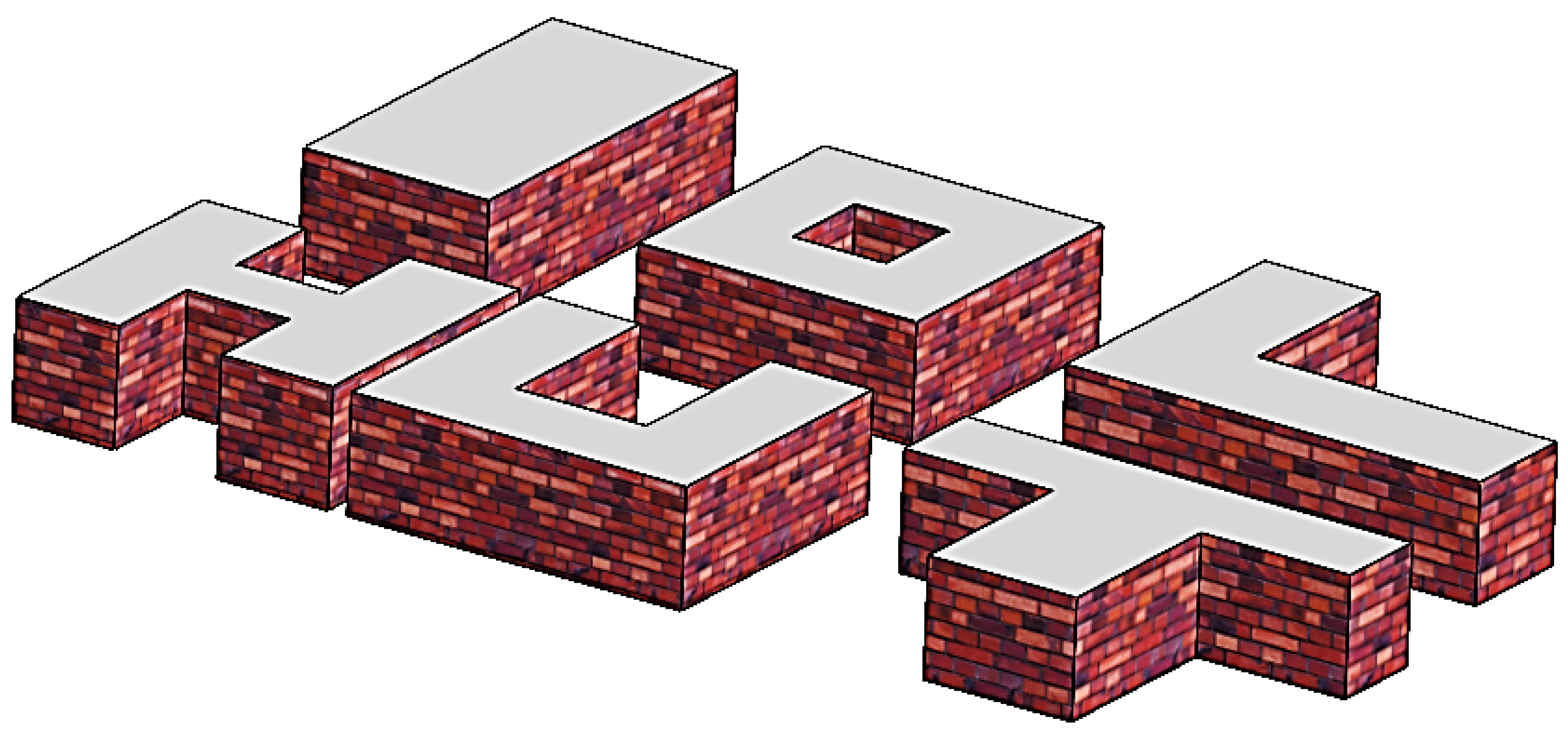
Before estimating the cooling load of any building, some basic information is necessary to design an appropriate HVAC system, like building location, orientation, weather conditions, building spacing, building materials, etc. The more exact the information is, the more accurate the load estimated will be. The shape of a building significantly impacts its energy performance and thermal comfort. Its shape depends on factors like the orientation, window-to-wall ratio, climate, and occupancy patterns. Common shapes include rectangle, L-shape, T-shape, U-shape, H-shape, and rectangle with interior-shape (see Figure 3). In fact, one of the goals of this study is to reduce the time required for thermal load calculations when there are multiple probabilities for the outcome of complex buildings. Several building applications, such as swimming pools, theatres, commercial buildings, stadiums, and residential buildings, impose restrictions. However, with the help of a specialized program called HAP that contains all these applications, it is easy to access accurate information. It can predict thermal loads for both simple and complex buildings. A rectangular building has less heat loss or gain through the walls, which reduces the heating and cooling loads. It also has less natural ventilation and daylight, requiring more mechanical systems. An L-shaped building offers more solar exposure and natural ventilation, increasing thermal comfort but increasing the heating and cooling loads. T-shaped and H-shaped buildings offer more solar exposure but may have disadvantages like increased heat loss, uneven loads, and increased cooling and structural loads. A U-shaped building creates a courtyard, improving thermal comfort but also increasing heating and cooling loads. The six building shapes used in this study were generated using the hourly analysis program (HAP) by Carrier. This is a specialized program for calculating cooling and heating loads and simulating buildings, which uses the transfer functions method and the heat balance method. These methods require a complex and lengthy data input compared with the basic version of calculating a cooling load using the transfer function method, which is to use the one-step procedure, which was first presented in the ASHRAE Handbook of Fundamentals in 2009 [29]. This method is called the cooling load temperature difference (CLTD) method. In this method, hand calculations are used to calculate the cooling load. Hand calculations are performed for a small portion of the building, and Figure 4 shows the dimensions. The buildings considered in this study are supposed to be located at 20.4 E longitude and 48.6 N latitude in Miskolc, Hungary at an elevation of about 130 m above mean sea level. In Miskolc, the summers are warm, the winters are cold and sometimes snowy, and it is partly cloudy year round. Over the course of the year, the temperature typically varies from −4 °C to 27 °C and is rarely below −11 °C or above 33 °C. The peak heating load for the winter occurred on December 14, when the outside temperature was −9 °C. The peak cooling load for the summer occurred on July 17, when the outside temperature was 34 °C. The inside temperature was always considered to be 22 °C.

All the buildings have the same floor area (200 m²) and height (6 m), thus the same volume (1200 m³). However, they have different shapes and therefore different wall surface areas and thus total surface areas. The materials used for each component of a building are the same for all building forms. The newest and most prevalent materials in the building construction sector, as well as those with the lowest U-value in walls (0.637 W/m²K), roofs (0.513 W/m²K), windows (3.123 W/m²K), floors (0.568 W/m²K), were used to make the sample buildings. These buildings were each simulated as residential dwellings in Miskolc. External heat gains arrive from the transfer of thermal energy from the outside hot medium to the inside space, mostly in summer. Heat transfer takes place via conduction through external walls, the top roof, and the bottom ground. Solar radiation heat travels as electromagnetic waves from the sun and enters the houses through windows and doors. The amount of solar radiation depends on the orientation of the windows and doors, the time of day and year, and the presence of shading devices. The overall shading coefficient is 0.870 [29], an indicator of how well the glass is thermally insulating (shading) the interior when there is direct sunlight on the window. Solar radiation can be beneficial for heating the house in the winter, but it frequently causes overheating in the summer. Ventilation is the transfer of heat through the movement of air between indoor and outdoor spaces. Ventilation can provide fresh air and improve indoor air quality, but it can also increase heat loss or gain depending on the temperature difference between indoor and outdoor air. The ventilation requirement is 0.3 L/s/m² [30] for residential dwelling unit applications. Infiltration is the movement of air through cracks and gaps in the building envelope. Heat can leak out of the building through poorly sealed windows and doors or enter through openings around pipes and wires. Infiltration can cause unwanted heat loss or gain, as well as moisture problems and air quality issues. The enter infiltration is taken for air change per hour (0.5 ACH) [31]. Other sources are internal heat generation, like in residential buildings with a maximum of ten occupants (40 W/m²), sedentary activities (67.4 W/m² sensible heat and 35.2 W/m² latent heat), miscellaneous loads (60 W/m² sensible heat and 55 W/m² latent heat), electric equipment (2.69 W/m²), and light (10.76 W/m²). Thermal characteristics were determined using mixed modes with 95% efficiency, a thermostat range of 24–18.3 °C, and 15–20 h of operation on weekdays and 10–20 h on weekends. Clearly, valid and sufficient data have been regarded as the essential tool to make the most use of the techniques proposed in this paper. Each input parameter corresponds to a different attribute of the structure. For example, the relative compactness (RC), which is the ratio of surface area to volume [32], is determined as follows [33]:

$$RC=6V^{2/3}{A}^{-1},$$

(1)

where A and V are the building surface area and volume, respectively. For a cuboid-shaped building, its value is unity, thus for any other rectangular building, it is smaller than 1.

The study compares the structure with and without windows. For the unglazed system, it analyzes six different building types with four orientations, which yields 24 cases. For the glazed system,

Table 1. The assumptions and conditions used to generate the database.

Features	Values and States
Number of building	6
orientations	4
Glazing areas	5 (5%, 10%, 15%, 20%, and 30%) of the floor area.
Distribution scenarios	5
Building volume	1200 m3

summarizes the used possibilities. There are six building shapes, depicted in Figure 4. There are four orientations of the building, N, E, S, or W. We examined five glazing areas, namely 5%, 10%, 15%, 20%, or 30% glazing area of the floor area. Five distribution scenarios were used in the study. Finally, we generated five window-distribution scenarios for each building shape, orientation, and glazing area. In each scenario, the windows were distributed into two of the five surfaces (N, E, S, W, and the horizontal roof), with half of the windows.

This results in 6 × 5 × 5 × 4 = 600 samples for the glazed system, thus the total number of the examined possibilities is 600 + 24 = 624. The study focuses on the residential buildings’ heating load and cooling load parameters, respectively. These parameters depend on seven factors: RC, exposed area, wall area, roof area, glazing area (which is the total area of the glazing including the frame and sash [34]), orientation, and glazing area distribution.

Table 2. The statistical analysis of energy-efficient design on eight features of the efficient building.

Characteristics	Mean	Median	Min.	Max.	Std. Deviation	Standard Error	Variance	Skewness
Direction	2.5	2.5	1	4	1.119	0.045	1.252	0.0
Dist. of AW	7.02	7	0.0	14	3.981	0.159	15.852	0.065
Exposed Area	633.73	648	500	716	53.818	2.154	2896.377	−1.021
Roof Area	193.08	200	140	200	11.260	0.451	126.793	−1.926
RC	0.678	0.658	0.5961	0.8537	0.0639	0.00256	0.004	1.316
Wall Area	440.65	453	300	516	53.645	2.148	2877.819	−1.044
Window Area	30.77	30	0	60	17.972	0.719	323.003	0.324
Cooling Load	24.4	23.5	14.5	42.7	5.7738	0.231	33.33	0.717
Heating Load	22	22	16.6	26.5	1.9871	0.0795	3.949	−0.058

summarizes the main statistical criteria used to analyze the data: mean, standard error, median, mode, standard deviation, sample variance, skewness, and minimum and maximum values.

3.2. The Main Equations

To estimate the thermal comfort of residents, this study applies intelligent models. The models’ accuracy is measured by three criteria: R², MAE, and RMSE. Previous research has extensively validated and confirmed these criteria. Equations (2)–(4) show the formulae for these criteria, which contrast the observed and predicted values of the thermal comfort [35].

$$R^2=1-\left[{\displaystyle \sum _{i=1}^N(}{Q}_{i_{predicted}}-Q_{i_{observed}}{)}^2/{\displaystyle \sum _{i=1}^N(}{Q}_{i_{observed}}-\overline{Q_{{}_{i_{observed}}}}{)}^2\right],$$

(2)

$$MAE=(1/N){\displaystyle \sum _{i=1}^N\left|Q_{i_{observed}}-Q_{i_{predicted}}\right|},$$

(3)

$$RMSE=\sqrt{(1/N){{\displaystyle \sum _{i=1}^N\left[Q_{i_{observed}}-Q_{i_{predicted}}\right]}}^2}.$$

(4)

The normalized root-mean-square deviation (NRMSD) depends on RMSE. The equations above show how to compare the actual and predicted values of HL or CL for an efficient building, which are denoted by $Q_{i_{observed}}$ and $Q_{i_{predicted}}$, respectively. The term N represents the total number of samples, and $Q_{{}_{i_{observed}}}$ is the average of the actual values of HL (or CL).

4. Results and Discussion

This study applied MLP and RB neural networks with three algorithms (LM, SCG, and RB) described in Section 2 to simulate the HL and CL of the residential building. The algorithms were implemented using MATLAB R2020b and IBM SPSS 20 statistics software. The dataset used to train the proposed network consisted of 624 samples, with seven independent factors affecting the HL and CL values, as explained earlier. A 70, 15, and 15 split was used to divide the data into training, testing, and validating sets, respectively. The performance of the models was evaluated using R², MAE, and RMSE, which are widely used in the literature [36]. To obtain the optimal structure of the models, an extensive trial and error process was conducted. The prediction results of each model for the HL and CL values were presented and discussed in detail.

To validate our results, we compared the predicted data with the experimental data collected by HAP, explained in Section 3.1, based on the CL and HL parameters. We used R² as a criterion for the predicted data. Figure 5 shows the comparison of the predicted data with the experimental data. The results indicate that the LM model has the best prediction performance among all models. The analytical results are also in good agreement with the experimental data, which confirms the reliability of the ANN training process using different algorithms. The RB model, however, has the lowest prediction accuracy and fails to optimize the ANN parameters effectively. The SCG model can be a suitable alternative to the LM model and provides accurate results and predictions, but it is still less accurate than the LM model. Figure 6 presents a graphical comparison between the predicted and actual values of HL and CL for each model. Figure 7 displays the histograms of the errors for each model and parameter. These figures illustrate the prediction capability of each model and the error distribution. The error analysis shows that the LM model has less error in prediction. Figure 6 also shows how close the experimental data and the prediction data are for each sample number using the LM, SCG, and RB models for HL and CL parameters. As mentioned before, we used the prediction data to verify the accuracy and validity of our analysis. Therefore, we compared the data of LM, SCG, and RB models for HL and CL parameters in detail and measured their deviation from the target data.

Table 3. Performance measures of the models for the HL parameter: RMSE, R², and MAE.

Models	RMSD	NRMSD	R2	MAE
LM	0.348	0.0157	0.973	0.273
SCG	0.371	0.0168	0.961	0.287
RB	0.746	0.0338	0.902	0.609

and

Table 4. Performance measures of the models for the CL parameter: RMSE, R², and MAE.

Models	RMSD	NRMSD	R2	MAE
LM	0.947	0.0388	0.93	0.682
SCG	1.226	0.0502	0.787	0.811
RB	2.185	0.0895	0.457	1.615

show the values of these criteria for each model and parameter. A lower RMSD value indicates a higher accuracy of the model. The LM model has the lowest RMSD values for both HL and CL parameters (0.348 and 0.947, respectively), which means it has the highest accuracy among all models. The RB model has the highest RMSD values and the lowest accuracy. The NRMSD value is another measure of accuracy, with a lower value indicating a better performance. The LM model has the lowest NRMSD values for both parameters, which confirms its superior performance. The R² value is a measure of how well the model fits the data, with a higher value indicating a better fit. Table 3 and Table 4 show that the LM model has the highest R² values for both parameters, which means it has the best fit to the data. The MAE value is a measure of the average error of the model, with a lower value indicating a smaller error. In the tables, the LM model has the lowest MAE values for both parameters (0.273 and 0.682, respectively), which means it has the smallest error among all models. Based on these results, we can conclude that the LM model is the best model for optimizing the ANN parameters and predicting the target data.

The thermal energy demand necessary to maintain an indoor comfort zone within a building is commonly referred to as the heating and cooling load. This load is subject to modification based on the architectural characteristics and design of the building. The heating and cooling demand is influenced by various factors, including but not limited to the building envelope, orientation, window-to-wall ratio, climate, and occupancy patterns.

The results of the analysis show that the heating and cooling loads vary significantly depending on the building shape (exposed area for wall, roof, and RC), orientation, glazing area, and glazing distribution. The results also show that there is a trade-off between minimizing the heating load in winter and minimizing the cooling load in summer. The results indicate that some building shapes are more efficient than others in terms of energy consumption and thermal comfort.

Our work concludes that the optimal building shape that balances the heating and cooling load close to the mean value is the L-shape shown in Figure 8. This is beneficial because it allows for the use of smaller and more efficient HVAC systems compared to all other shapes except the rectangular one. This can lead to lower energy costs and reduced carbon dioxide emissions. Additionally, having a balanced heating and cooling load can help maintain a comfortable indoor environment by reducing temperature fluctuations [37]. Also, the best orientation for this shape is south, which allows maximum solar gain in winter. The design area has a moderately cold climate that requires heating for about half of the year. Furthermore, the best glazing area for this shape is 20%, which provides sufficient daylight and ventilation without causing excessive heat loss or gain. From this point of view, the L-shape is better than the rectangular shape. Finally, the best glazing distribution for this shape is on the east and south sides, which optimizes the solar exposure and shading effects throughout the day. In this case, the building has a heating load of 22.5 kWh and a cooling load of 24.5 kWh for the temperatures given in Section 3.1, which are both close to the mean values in Table 2 of 22 kWh and 24.4 kWh, respectively. This model’s heating and cooling values are the closest to the mean value compared to the other 624 models.

5. Numerical Simulation

The final part of this research numerically simulates the walls of this building for the winter and summer seasons based on the peak load of each season. The simulation does not include other components that affect the heating and cooling load, such as the roof, ventilation, leakage, glass load, and internal loads from people, lighting, etc. These factors are only considered in the steady-state case. The transient simulation uses December and July as representative months.

5.1. The Equation and Its Discretization

We can describe how heat moves inside a solid material that has homogeneous properties and also has a source of heat using a type of equation called a linear parabolic PDE. This Equation (5) is based on the simplest form of Fourier’s law of heat conduction.

$$\frac{\mathsf{\partial }u}{\mathsf{\partial }t}=\alpha {\nabla }^{2}u+q,$$

(5)

where q represents the amount of heat that is generated or added to the material, $u=u\left(\overrightarrow{r},t\right)$ is the temperature, and α is the thermal diffusivity, which is given as $\alpha =k/(c\rho )$, where $k=k\left(\overrightarrow{r},t\right)$, $c=c\left(\overrightarrow{r},t\right)$, and $\rho =\rho \left(\overrightarrow{r},t\right)$ are the thermal conductivity, specific heat, and the density of the material, respectively.

Convection, which is the heat transfer between the material and the surrounding air, depends on the difference between the temperature of the material u and the temperature of the air u_a. Newton’s law of cooling suggests that a term $K\left(u_a-u\right)$ can describe convective heat transfer [38]. Consequently, it makes sense to include the $K{u}_a$ term in the expression q, which represents the heat source. The radiation heat loss depends on the fourth power of the temperature of the material u. The expression for radiation includes the proportionality constant σ, which is related to the Stefan–Boltzmann constant and the surface area [39]. The term $-\sigma u^4$ can represent the amount of heat that a surface area loses by radiation. The proportionality constant σ is now equal to the Stefan–Boltzmann constant multiplied by the surface area in [k/s], so we divided it by $(c\rho .\Delta x)$ to obtain the heat loss in [W]. The heat source q, convection term K, and the outgoing radiation $-\sigma u^4$ can be combined and added to the heat source q in the heat conduction equation., which also has a term α that describes how well the material can conduct and store heat. The extended equation is:

$$\frac{\mathsf{\partial }u}{\mathsf{\partial }t}=\frac{1}{\rho \left(x\right)c\left(x\right)}\nabla (k\left(x\right)\nabla u)+q.$$

(6)

where $u=u(\overrightarrow{r},t)$ is the temperature in Kelvin, t is the time in seconds, and q is the heat generation in K/s.

A wall segment with an area of 1 m² is examined, where the temperature is supposed to change only along the x direction. It means that although we simulate a 3D domain, mathematically we have a 1D problem. The number of cells in the y and z direction was 1, so $\Delta y=\Delta z=1$ and the volume of a cell is $\Delta x$. The space is divided to obtain a one-dimensional array of cells with cell centers, $\left(x_i\right)=\left(i-\raisebox{1ex}{$1$}\!\left/ \!\raisebox{-1ex}{$2$}\right.\right)\Delta x,\hspace{0.33em}i=1,\dots ,N$, where N is the overall number of cells. Since the material boundaries are always positioned onto the cell borders, the average conductivity $\left(k_i+k_{i+1}\right)/2$ can be used between the two neighboring cells to describe heat conduction between them. By applying the central difference formula in one dimension, we can obtain the following spatially discretized form of Equation (6):

$$\frac{d{u}_i}{dt}=\frac{1}{c_i{\rho }_i\Delta x} \left(\frac{k_i+k_{i+1}}{2}\frac{u_{i+1}-u_i}{\Delta x}+\frac{k_i+k_{i-1}}{2}\frac{u_{i-1}-u_i}{\Delta x}\right)\hspace{0.17em}+q-K{u}_i-\sigma u_i{}^4,$$

(7)

where $u_i ,\hspace{0.33em}{\rho }_i$, and $c_i$ are cell variables. The heat capacity of the cell is $C_i=c_i{\rho }_i{V}_i=c_i{\rho }_i\Delta x$. The thermal resistance in the x-direction between two cells has the approximate equation $R_{i,i+1}\approx \Delta x/k_{i,i+1}$ between two adjacent cells with the same material. If the material properties are different, we can write for the resistance between two cells i and i + 1 that $R{x}_{i,\hspace{0.17em}i+1}\approx \frac{2\Delta x}{k_i+k_{i+1}}$. Then, we can use these quantities to write an equation for how each cell variable changes over time.

$$\frac{d{u}_i}{dt}=\frac{u_{i-1}-u_i}{R_i{{}_{-1,}}_i{C}_i}+\frac{u_{i+1}-u_i}{R_i{{}_{+1,}}_i{C}_i}+q-K{u}_i-\sigma u_i{}^4$$

(8)

5.2. The Leapfrog–Hopscotch Structure

The leapfrog–hopscotch algorithm is a finite difference method that can be used to simulate complex 1D, 2D, and 3D models. It is capable of working with both stiff and non-stiff systems that may involve compound materials, regardless of whether the spatial mesh is equidistant or non-equidistant. To use the leapfrog–hopscotch algorithm, we need to divide the space domain into two different subgroups using a special type of mesh called a bipartite mesh. The cells or nodes in the first subgroup are odd, and the ones in the second subgroup are even. The main rule is that, like on a chessboard, all the neighboring cells of an odd cell must be even and vice versa. We can illustrate this with a 1D interval $x\in \left[x_0\hspace{0.17em},\hspace{0.17em}{x}_N\right]$, $L=\hspace{0.17em}{x}_N-x_0$ on which coordinates are used to create an equidistant grid $x_0\hspace{0.17em}, x_1\hspace{0.17em}, \dots ,\hspace{0.17em}\hspace{0.17em}{x}_N$ of nodes, so $x_j=x_{j-1}+\Delta x ,\hspace{0.17em} \hspace{0.17em}j=1,\dots ,N,\hspace{0.33em}\hspace{0.17em}\Delta x=L/N\hspace{0.17em}$. The time domain is $t\in \left[t^0,\hspace{0.17em} t^{\mathrm{fin}}\right]$, and it is discretized as usual: $t^j=t^0+jh\hspace{0.17em},\hspace{0.33em}\hspace{0.17em}j=1,\dots ,\hspace{0.17em} T\hspace{0.17em},\hspace{0.33em}\hspace{0.17em}hT=t^{\mathrm{fin}}-t^0$, where h is the time step size.

Figure 9 illustrates the space–time structure of the leapfrog–hopscotch (LH) method [18]. The method has two half- and several full-time steps. The first step is a half-time step for the odd nodes, using the initial values. This is shown by a blue half-rectangle in the figure. Then, the method alternates full-time steps (red rectangle in the figure) for the even and odd nodes until the end. The last step is a half-time step for the odd nodes, to match the final time point of the even nodes. This is shown by a blue half-rectangle in the figure. The key point is that when we calculate the value of node i, we use the latest values of its neighbors i − 1 and i + 1 in the equations.

As we showed in the introduction of our previous paper [17], the following set of formulas are quite effective to solve Equation (8). The first stage is half of the time step to update the values of the odd nodes with the formula:

$$u_i^{\raisebox{1ex}{$1$}\!\left/ \!\raisebox{-1ex}{$2$}\right.}=\frac{u_i^0+A_i^0/2-K\Delta t{u}_i^0/4}{1+r_i+K\Delta t/4+\sigma \Delta t{\left(u_i^0\right)}^3/2}$$

(9)

Then, a full time step stage is calculated as

$$u_i^1=\frac{u_i^0+A_i^{1/2}-K\Delta t{u}_i^0/2}{1+r_i+K\Delta t/2+\sigma \Delta t{\left(u_i^0\right)}^3}$$

(10)

where

$$A_i^n=\Delta t{\displaystyle \sum _i\frac{u_i^n}{R_i{C}_i}}\hspace{0.17em}+\Delta t\cdot q_i, \mathrm{and} r_i=\Delta t{\displaystyle \sum _i\frac{1}{R_i{C}_i}}\hspace{0.33em},\hspace{0.33em}\hspace{0.33em}i=1, \dots ,N ,\hspace{0.33em}\hspace{0.17em}n=0,\hspace{0.17em}1/2.$$

The first variable represents the collective effect of the temperature of neighboring cells on cell i. The second quantity can be thought of as an extension of the mesh ratio, which is commonly used as $r=\frac{\alpha \Delta t}{\Delta x^2}$. More precisely, the relationship remains valid for Equation (8), where $r_i=2r$. Equation (10) is applied until the last stage as well, but then the time step size must be halved.

Geometry and Material Properties

A cross-section of a wall is considered with dimensions 42 cm in the x and 100 cm in the y and z direction, as can be seen in Figure 10. The four layers consist of gypsum plaster, heavy weight concrete, insulation, and face brick. This wall structure is the same and has the same U value as used in Section 3.1.

In the current work, the real material properties listed in

Table 5. The properties of the materials used were taken from HAP based on ASHRAE Standard [29].

Layers	Thickness (cm)	$\mathit{\rho }\hspace{0.33em}\left(\mathbf{k}\mathbf{g}{\mathbf{m}}^{-3}\right)$	$\mathit{c}\left(\mathbf{J}\mathbf{k}{\mathbf{g}}^{-1}{\mathbf{K}}^{-1}\right)$	$\mathit{k}\left(\mathbf{W}{\mathbf{m}}^{-1}{\mathbf{K}}^{-1}\right)$
Gypsum plaster	2	1601.8	840	0.726
HW concrete	25	2242.6	840	1.73
Insulation	5	91.3	840	0.043
Face brick	10	2082.4	920	1.3

are taken into account. Note that these coefficients are constants inside a material, that is, they do not change with time, space, or temperature, but they have a discontinuity at the border of the materials.

5.3. Mesh Construction, Initial and Boundary Conditions

In our one-dimensional simulation, we assumed that the wall thickness is 42 cm. To test the independence of the results on mesh density, nine meshes with an increasing number of cells along the x-axis were used for the four layers of wall starting from $\Delta x_i=1.0 \mathrm{cm}$ (Nx = 42) until $\Delta x_i=0.1 \mathrm{cm}$ (N = 420). The heat loss was calculated according to the number of cells. Figure 11 shows that when we increase the number of cells to more than 336, the heat loss remains approximately the same. Therefore, we chose that mesh with $\Delta x_i=0.125 \mathrm{cm}$, where the number of cells in each layer was $N_1=16, N_2=200, N_3=40$, and $N_4=80$. The simulation time is one month for the winter season and for the summer, and both contain 31 days, thus $t_{\mathrm{fin}}=2,678,400\mathrm{s}$ serves as the final time (the end of the examined time period). The duration of each time step is also expressed in seconds, first with $h=100\mathrm{s}$.

Convective and radiation heat transfer occur in the x-direction, which is the direction of heat transfer depicted in Figure 10.

Table 6. Convection, radiation, and heat source parameters are present on both sides of the wall during the winter season [40].

	${\mathit{h}}_{\mathit{c}}$$\left[\frac{\mathbf{W}}{{\mathbf{m}}^2\mathbf{K}}\right]$	Temperature [K]	ε	${\mathit{\sigma }}^{\ast }$$\left[\frac{\mathbf{W}}{{\mathbf{m}}^2{\mathbf{K}}^4}\times 10^{-8}\right]$
Inside condition	8.3	295	0.9	5.1
Outside condition	0.6–19.6	264–284	0.9	5.1

summarizes the boundary inside and outside condition of heat transfer for winter season convection coefficients ($h_c$), temperature and emissivity (ε) of the surfaces for the inside constant conditions and for the outside changing with time depending on the ambient conditions. The inside boundary condition is taken to be the constant comfort zone, which is taken from [29]. The outside condition changes with time depending on the changing weather conditions. The ambient air temperature, velocity, and the total solar radiation are taken according to real weather conditions in Miskolc city from 1st December 00.0 a.m. to 31st December 00.0 p.m. [40].

Table 7. Convection, radiation, and heat source parameters are present on both sides of the wall during the summer season [40].

	${\mathit{h}}_{\mathit{c}}$$\left[\frac{\mathbf{W}}{{\mathbf{m}}^2\mathbf{K}}\right]$	Temperature [K]	ε	${\mathit{\sigma }}^{\ast }$$\left[\frac{\mathbf{W}}{{\mathbf{m}}^2{\mathbf{K}}^4}\times 10^{-8}\right]$
Inside condition	8.3	295	0.9	5.1
Outside condition	2.7–16.9	284.2–307	0.9	5.1

shows the boundary condition for the summer season and the data are taken according to real weather conditions in Miskolc city from 1 July 00.0 a.m. to 31 July 00.0 p.m. [40].

We obtain the values of the coefficients in our equations as follows: [38],

$$K=\frac{h_c}{c\rho \Delta x}\hspace{0.17em},\hspace{0.33em}\hspace{0.17em}\sigma =\frac{{\sigma }^{\ast }}{c\rho \Delta x}\hspace{0.17em},\hspace{0.33em}\hspace{0.17em}{\sigma }^{\ast }=5.678\ast {10}^{-9}\ast \epsilon , q=\frac{q^{\ast }}{c\rho \Delta x}+\frac{h_c}{c\rho \cdot \Delta x}\cdot u_{\mathrm{a}}.$$

We also supposed that the inside and outside elements have heat sources as follows:

$$For\; the\; inside\; elements:q_{in}=\frac{1}{c\rho }\times q_{in}^{\ast }+\frac{h_{cin}}{c\rho \cdot \Delta x}\times u_{in}$$

$$For\; the\; outside\; elements:q_{\mathrm{out}}(t)=\frac{1}{c\rho }\times q_{\mathrm{out}}^{\ast }\left(t\right)+\frac{h_{c\mathrm{out}}\left(t\right)}{c\rho \cdot \Delta x}\times u_{\mathrm{out}}\left(t\right)$$

$$\mathrm{And} K\left(t\right)=\frac{h_{c\mathrm{out}}\left(t\right)}{c\rho \Delta x}\hspace{0.17em},\hspace{0.33em}\hspace{0.17em}\sigma =\frac{{\sigma }_{\mathrm{out}}{}^{\ast }}{c\rho \Delta x}\hspace{0.17em},\hspace{0.33em}\hspace{0.17em}q\left(t\right)=\frac{q_{\mathrm{out}}{}^{\ast }\left(t\right)}{c\rho \Delta x}+\frac{h_{c\mathrm{out}}\left(t\right)}{c\rho \cdot \Delta x}\cdot u_{\mathrm{out}}\left(t\right)$$

where $q_{in}^{\ast }={\epsilon }_{in}{\sigma }_{in}{(u_{in})}^4$ and $q_{\mathrm{out}}^{\ast }\left(t\right)={\alpha }_{\mathrm{sun}}{G}_{c\mathrm{out}}\left(t\right)+{\alpha }_{\mathrm{Low}}{\epsilon }_{\mathrm{out}}{\sigma }_{\mathrm{out}}{\left[u_{\mathrm{out}}\left(t\right)\right]}^4$ [41].

The convection heat transfer coefficient for outside elements as a function of air velocity is estimated as follows [42]:

$$h_{c\mathrm{out}}\left(t\right)=0.6+6.64\sqrt{v(t)}\hspace{0.17em}$$

$v\left(t\right)$: The air velocity [40] is taken every 100 s in December and July [m/s].

• $u_{\mathrm{out}}\left(t\right)$: The outside air temperature is taken every 100 s in December and July [°C].
• $u_{in}$: The inside air temperature [°C] on the left side.
• $G_{c\mathrm{out}}\left(t\right)$: The solar radiation is taken every 100 s in December and July [W/m²]. The website gives four $G_{c\mathrm{out}}\left(t\right)$ functions, one for each orientation of a vertical wall.
• ${\alpha }_{\mathrm{sun}}$: The absorptivity of brick surface to solar radiation, which is taken as 0.9.
• ${\alpha }_{\mathrm{Low}}$: The absorptivity of brick surface to low-temperature thermal radiation, which is taken as 0.9.

The environment air temperature is taken to be $22 °\mathrm{C}\approx 295 \mathrm{K}$ inside, and changes depending on weather conditions outside.

We calculated the initial temperature inside the wall using the assumption that before the simulation time, a stationary heat flow with constant flux evolved between the given boundary values of the inside and outside air temperatures. For example, in the case of one layer, it yields a linear function of the x variable for the initial condition:

$$u\left(x,\hspace{0.33em}t=0\right)=(u_{\mathrm{out},\mathrm{initial}}-u_{in})x/L_x+u_{in},$$

where $u_{\mathrm{out},\mathrm{initial}}=264 \mathrm{K}$ for the winter season, and for the summer season $u_{\mathrm{out},\mathrm{initial}}=307 \mathrm{K}$.

For the multi-layer wall case, the assumption of stationary heat conduction with the initial values at the boundaries implies that we have to use piecewise linear functions of the x variable for the initial condition:

$$\begin{gathered} q_{\mathrm{flux}}=(u_{\mathrm{out},\mathrm{initial}}-u_{in})/{\displaystyle \sum _{i=1}^{i=4}\frac{L_i}{K_i}}, \\ \mathrm{where} u_{\mathrm{initial},\mathrm{Layer},i+1}=u_i-(q_{\mathrm{flux}}{L}_i/k_i). \end{gathered}$$

5.4. Result for the Simulation of the Wall

5.4.1. Winter Simulation

This paragraph presents the results of a simulation of heat transfer and temperature distribution in a four-layered wall during the winter season (December). The simulation shows how the temperature varies across the layers and how much heat is lost from the inside to the outside of the wall per meter square. Figure 12, Figure 13, Figure 14 and Figure 15 show the temperature distribution at the boundary surfaces of the layers when the wall faces North, East, South, and West directions, respectively. The following observations can be made from the results. The inside surface temperature (gypsum plaster) and the first cell of the HW concrete layer are close to the inside air temperature, indicating that these layers insulate from the outside and do not store much heat.

The first cell of the insulation layer and the outside surface temperature (brick) are close to the outside air temperature, indicating that the insulation layer has a low thermal conductivity and reduces the heat loss by storing heat.

The North-facing wall has the largest temperature gradient and the highest heat loss because it does not receive any solar radiation. For the South-facing wall, the opposite is true. The East-facing and West-facing walls have approximately similar temperature gradients and heat losses because they receive approximately similar amounts of solar radiation. They are intermediate between the North-facing and South-facing walls, but the east wall is slightly colder than the west wall.

Figure 16 shows that the heat loss per meter squared is the highest for the wall facing North and lowest for the wall facing South.

5.4.2. Summer Simulation

This section shows the results of a simulation of heat transfer and temperature distribution in the four-layered wall during the summer season (July), depicted in Figure 10. The simulation shows how the temperature varies across the layers and how much heat is gained from the outside to the inside of the wall per meter squared. Figure 17, Figure 18, Figure 19 and Figure 20 show the temperature distribution at the boundary surfaces of the layers when the wall faces North, East, South, and West directions, respectively. The following observations can be made from the results.

The inside surface temperature (gypsum plaster) and the first cell of the HW concrete layer are close to the inside air temperature, indicating that these layers have a high thermal conductivity and do not store much heat.

The first cell of the insulation layer and the outside surface temperature (brick) are higher than the outside air temperature during nights, indicating that the insulation layer has a low thermal conductivity and increases the heat gain by storing heat received during the daytime. But in the case of the East, West, and especially the South wall, the surface temperature can be higher even during the daytime due to solar radiation and the rather high emissivity.

The North-facing wall has the smallest temperature gradient and the lowest heat gain because it does not receive a significant amount of solar radiation. The opposite is true for the South-facing wall. The East-facing and West-facing walls are between the North-facing and South-facing walls, but surprisingly, the East-facing wall has noticeably higher temperatures and heat gain than the West wall.

Figure 21 illustrates that the heat gain per meter squared is lowest for the wall facing North and highest for the wall facing South.

The wall simulation presents how the temperature varies in °C on the South-facing side of the building. Figure 22 displays the contour of the temperature distribution for two different seasons: winter (left) and summer (right). The simulation results are based on the last midnight of December and July, respectively. One can notice the heat stored by the wall during the summer night.

Table 8. The heat loss and heat gain in transient method by LH and steady-state method by HAP.

Methods	Winter				Summer
	Heat Loss [kW/m2]				Heat Gain [kW/m2]
Direction	N	E	S	W	N	E	S	W
LH	17.34	17.16	16.92	17.08	−3.45	−9.745	−12.09	−5.99
HAP	19.35	19.44	19.35	19.43	−4.7	−7.65	−7.8	−7.43
percentage difference	2.7%	3.1%	3.3%	3.2%	7.6%	6.0%	10.7%	5.3%

summarizes the heat loss and gain for the wall based on the simulation and HAP peak load, i.e., for the coldest and hottest days, respectively. The heat loss is the highest in winter on December 14, and the heat gain is the highest in summer on 17 July.

The transient simulation by LH is more realistic and accurate because it uses real data from the weather website [40] for 2022 and 2023. The steady-state method by HAP is based on the location, design temperature for winter and summer, and estimated factors that increase the load to avoid underdesign. The steady-state values are always higher in winter than the transient simulation values.

6. Conclusions

This study applied and compared MLP and RB neural networks with three algorithms (LM, SCG, and RB) to estimate the HL and CL of a residential building. The buildings were located in Miskolc, Hungary. The walls of the buildings consisted of gypsum plaster, HW concrete, insulation, and brick layers. The models were developed and assessed using 624 samples with seven independent factors. The accuracy and error of the models were evaluated by R², MAE, RMSE, RMSD, and NRMSD. The results revealed that the LM model outperformed the other models in terms of prediction accuracy and error minimization. The LM model also had the best fit to the experimental data; notice that in the histogram figures, the error is approaching zero compared to the other algorithms, which verified the validity of the MLP training process. This study demonstrated that the MLP neural network with the LM algorithm can be an effective method for simulating the HL and CL of residential buildings.

In the simulation part, we investigated the thermal behavior of the same four-layered wall with different orientations in winter and summer by using the finite difference leapfrog–hopscotch algorithm coded in MATLAB. The simulation results showed the variation of temperature and heat transfer across the layers and the effect of solar radiation on the wall performance. The results revealed that the insulation layer played a key role in reducing the heat loss in winter and decreasing the heat gain in summer. The results also indicated that the wall orientation had a significant influence on the thermal performance, with the North-facing wall being the most efficient in summer and the South-facing wall being the most efficient in winter. The West- and East-oriented walls are intermediate between the North and the South, but surprisingly, the East wall has noticeably higher temperatures and heat gain in summer than the West wall. The simulation process confirmed that the steady-state calculations for the most extreme day of the winter overestimate the heat loss. On the other hand, on the hottest day of summer, the steady-state method can under- or overestimate the heat gain depending on the orientation of the wall. This study showed how wall design and orientation can optimize the thermal comfort of a building. Our next work will simulate the windows and the roof and we will use ANNs to solve the transient PDE itself, similarly to the work [43].

References

1. Chegari, B.; Tabaa, M.; Simeu, E.; Moutaouakkil, F.; Medromi, H. Multi-Objective Optimization of Building Energy Performance and Indoor Thermal Comfort by Combining Artificial Neural Networks and Metaheuristic Algorithms. Energy Build. 2021, 239, 110839. [Google Scholar] [CrossRef]
2. Feng, F.; Fu, Y.; Yang, Z.; O’Neill, Z. Enhancement of Phase Change Material Hysteresis Model: A Case Study of Modeling Building Envelope in EnergyPlus. Energy Build. 2022, 276, 112511. [Google Scholar] [CrossRef]
3. Winkelmann, F.C.; Selkowitz, S. Daylighting Simulation in the DOE-2 Building Energy Analysis Program. Energy Build. 1985, 8, 271–286. [Google Scholar] [CrossRef]
4. Beausoleil-Morrison, I.; Kummert, M.; MacDonald, F.; Jost, R.; McDowell, T.; Ferguson, A. Demonstration of the New ESP-r and TRNSYS Co-Simulator for Modelling Solar Buildings. Energy Procedia 2012, 30, 505–514. [Google Scholar] [CrossRef]
5. Rashad, M.; Żabnieńska-Góra, A.; Norman, L.; Jouhara, H. Analysis of Energy Demand in a Residential Building Using TRNSYS. Energy 2022, 254, 124357. [Google Scholar] [CrossRef]
6. Chen, R.; Tsay, Y.S.; Zhang, T. A Multi-Objective Optimization Strategy for Building Carbon Emission from the Whole Life Cycle Perspective. Energy 2023, 262, 125373. [Google Scholar] [CrossRef]
7. Zhou, G.; Moayedi, H.; Bahiraei, M.; Lyu, Z. Employing Artificial Bee Colony and Particle Swarm Techniques for Optimizing a Neural Network in Prediction of Heating and Cooling Loads of Residential Buildings. J. Clean. Prod. 2020, 254, 120082. [Google Scholar] [CrossRef]
8. Lu, C.; Li, S.; Penaka, S.R.; Olofsson, T. Automated Machine Learning-Based Framework of Heating and Cooling Load Prediction for Quick Residential Building Design. Energy 2023, 274, 126689. [Google Scholar] [CrossRef]
9. Khajavi, H.; Rastgoo, A. Improving the Prediction of Heating Energy Consumed at Residential Buildings Using a Combination of Support Vector Regression and Meta-Heuristic Algorithms. Energy 2023, 272, 127069. [Google Scholar] [CrossRef]
10. Chen, X.; Cao, B.; Pouramini, S. Energy Cost and Consumption Reduction of an Office Building by Chaotic Satin Bowerbird Optimization Algorithm with Model Predictive Control and Artificial Neural Network: A Case Study. Energy 2023, 270, 126874. [Google Scholar] [CrossRef]
11. Bagheri-Esfeh, H.; Safikhani, H.; Motahar, S. Multi-Objective Optimization of Cooling and Heating Loads in Residential Buildings Integrated with Phase Change Materials Using the Artificial Neural Network and Genetic Algorithm. J. Energy Storage 2020, 32, 101772. [Google Scholar] [CrossRef]
12. Jaber, A.A.; Saleh, A.A.M.; Ali, H.F.M. Prediction of Hourly Cooling Energy Consumption of Educational Buildings Using Artificial Neural Network. Int. J. Adv. Sci. Eng. Inf. Technol. 2019, 9, 159. [Google Scholar] [CrossRef]
13. Martínez-Comesaña, M.; Febrero-Garrido, L.; Granada-álvarez, E.; Martínez-Torres, J.; Martínez-Mariño, S. Heat Loss Coefficient Estimation Applied to Existing Buildings through Machine Learning Models. Appl. Sci. 2020, 10, 8968. [Google Scholar] [CrossRef]
14. Amiri, S.; Mazaheri, M.; Bavandpouri Gilan, N. Introducing a New Method for Calculating the Spatial and Temporal Distribution of Pollutants in Rivers. Int. J. Environ. Sci. Technol. 2021, 18, 3777–3794. [Google Scholar] [CrossRef]
15. Jejeniwa, O.A.; Gidey, H.H.; Appadu, A.R. Numerical Modeling of Pollutant Transport: Results and Optimal Parameters. Symmetry 2022, 14, 2616. [Google Scholar] [CrossRef]
16. Kusuda, T. Fundamentals of Building Heat Transfer. J. Res. Natl. Bur. Stand. 1977, 82, 97. [Google Scholar] [CrossRef] [PubMed]
17. Askar, A.H.; Omle, I.; Kovács, E.; Majár, J. Testing Some Different Implementations of Heat Convection and Radiation in the Leapfrog-Hopscotch Algorithm. Algorithms 2022, 15, 400. [Google Scholar] [CrossRef]
18. Omle, I.; Askar, A.H.; Kovács, E.; Bolló, B. Comparison of the Performance of New and Traditional Numerical Methods for Long-Term Simulations of Heat Transfer in Walls with Thermal Bridges. Energies 2023, 16, 4604. [Google Scholar] [CrossRef]
19. Khakre, V.; Wankhade, A.; Ali, M.A. Cooling Load Estimation by CLTD Method and Hap 4.5 for an Evaporative Cooling System. Int. Res. J. Eng. Technol. 2017, 4, 1457–1460. [Google Scholar]
20. Askar, A.H.; Kovács, E.; Bolló, B. ANN Modeling for Thermal Load Estimation in a Cabin Vehicle. In Vehicle and Automotive Engineering 4: Select Proceedings of the 4th VAE2022; Springer: Miskolc, Hungary, 2022; pp. 357–373. [Google Scholar]
21. Mcculloch, W.S.; Pitts, W. A Logical Calculus Nervous Activity. Bull. Math. Biol. 1990, 52, 99–115. [Google Scholar] [CrossRef]
22. Fan, X.; Wang, L.; Li, S. Predicting Chaotic Coal Prices Using a Multi-Layer Perceptron Network Model. Resour. Policy 2016, 50, 86–92. [Google Scholar] [CrossRef]
23. Zarei, T.; Behyad, R. Predicting the Water Production of a Solar Seawater Greenhouse Desalination Unit Using Multi-Layer Perceptron Model. Sol. Energy 2019, 177, 595–603. [Google Scholar] [CrossRef]
24. Mlp, M.P.; Heidari, M.; Shamsi, H. Analog Programmable Neuron and Case Study on VLSI Implementation of Multi-Layer Perceptron (MLP). Microelectron. J. 2019, 84, 36–47. [Google Scholar] [CrossRef]
25. Sahib, M.M.; Kovács, G. Using Artificial Neural Network in the Reverse Design of a Composite Sandwich Structure. Struct. Eng. Mech. 2023, 85, 635. [Google Scholar]
26. Al-haddad, L.A. An Intelligent Fault Diagnosis Approach for Multirotor UAVs Based on Deep Neural Network of Multi-Resolution Transform Features. Drones 2023, 7, 82. [Google Scholar] [CrossRef]
27. Kanthasamy, R.; Witoon, T.; Abdullah, S. Process Intensification of Hydrogen Production by Catalytic Steam Methane Reforming: Performance Analysis of Multilayer Perceptron-Artificial Neural Networks and Nonlinear Response Surface Techniques. Process Saf. Environ. Prot. 2021, 156, 315–329. [Google Scholar] [CrossRef]
28. De Jesús, J.; Garcia, D.; Sossa, H.; Garcia, I.; Zacarias, A.; Mujica-vargas, D. Energy Processes Prediction by a Convolutional Radial Basis Function Network. Energy 2023, 284, 128470. [Google Scholar] [CrossRef]
29. Spitler, J.D. Load Calculation Applications Manual, Si ed.; Printed in the United States of America; ASHRAE: Peachtree Corners, GA, USA, 2009; ISBN 978-1-936504-76-3. [Google Scholar]
30. Liaison, S.; Emmerich, S.J.; Hedrick, R.L.; Mcfarland, J.K.; Aguilar, H.; Berlin, G.L.; Brunner, G.; Buttner, M.P.; Chisholm, J.K.; Damiano, L.A.; et al. Ventilation for Acceptable Indoor Air Quality. ANSI/ASHRAE Addenda h and l to, ANSI/ASHRAE Standard 62.1-2010, 2012; ISSN 1041-2336. 2012. Available online: https://www.ashrae.org/file%20library/technical%20resources/standards%20and%20guidelines/standards%20addenda/62_1_2010_h_l_final.pdf (accessed on 19 October 2023).
31. Sherman, M. Infiltration in ASHRAE’s Residential Ventilation Standards Infiltration in ASHRAE’s Residential Ventilation Standards; Lawrence Berkeley National Lab.: Berkeley, CA, USA, 2008. [Google Scholar]
32. Ouarghi, R.; Krarti, M. Building Shape Optimization Using Neural Network and Genetic Algorithm Approach. Ashrae Transactions 2006, 112, 484–492. [Google Scholar]
33. Xu, Y.; Li, F.; Asgari, A. Prediction and Optimization of Heating and Cooling Loads in a Residential Building Based on Multi-Layer Perceptron Neural Network and Different Optimization Algorithms. Energy 2022, 240, 122692. [Google Scholar] [CrossRef]
34. Huang, Y.; Niu, J.; Chung, T. Comprehensive Analysis on Thermal and Daylighting Performance of Glazing and Shading Designs on Office Building Envelope in Cooling-Dominant Climates. Appl. Energy 2014, 134, 215–228. [Google Scholar] [CrossRef]
35. Wu, Y.; Xie, P.; Dahlak, A. Utilization of Radial Basis Function Neural Network Model for Water Production Forecasting in Seawater Greenhouse Units. Energy Rep. 2021, 7, 6658–6676. [Google Scholar] [CrossRef]
36. Mosallanezhad, M.; Moayedi, H. Developing Hybrid Artificial Neural Network Model for Predicting Uplift Resistance of Screw Piles. Arab. J. Geosci. 2017, 10, 479. [Google Scholar] [CrossRef]
37. Burdick, A. Strategy Guideline: Accurate Heating and Cooling Load Calculations. In Building America Building Technologies Program Office of Energy Efficiency and Renewable Energy; U.S. Department of Energy: Washington, WA, USA, 2011; pp. 1–47. [Google Scholar]
38. Holman, J.P. Heat Transfer, 10th ed.; McGraw-Hill Education: New York, NY, USA, 2010. [Google Scholar]
39. Askar, A.H.; Nagy, Á.; Barna, I.F.; Kovács, E. Analytical and Numerical Results for the Diffusion-Reaction Equation When the Reaction Coefficient Depends on Simultaneously the Space and Time Coordinates. Computation 2023, 11, 127. [Google Scholar] [CrossRef]
40. Weather-Online Website. Available online: https://open-meteo.com (accessed on 1 April 2023).
41. Omle, I.; Kovács, E.; Bolló, B. Applying Recent Efficient Numerical Methods for Long-Term Simulations of Heat Transfer in Walls to Optimize Thermal Insulation. Results Eng. 2023, 20, 101476. [Google Scholar] [CrossRef]
42. Duffie, J.A.; Beckman, W.A. Solar Engineering of Thermal Processes; Wiley: New York, NY, USA, 1980. [Google Scholar]
43. Savović, S.; Ivanović, M.; Min, R. A Comparative Study of the Explicit Finite Difference Method and Physics-Informed Neural Networks for Solving the Burgers’ Equation. Axioms 2023, 12, 982. [Google Scholar] [CrossRef]
Figure 1. A schematic diagram of the ANN and its relation to the input and output parameters.
Buildings 13 02862 g001
Figure 2. The flowchart presents the process used to determine the prediction.
Buildings 13 02862 g002
Figure 3. Different shapes of the buildings.
Buildings 13 02862 g003
Figure 4. Dimensions of the buildings.
Buildings 13 02862 g004
Figure 5. The result of R2 values for the data predicted by three neural networks: MLP_LM, MLP_SCG, and RB (a) for the heating load and (b) for the cooling load.
Buildings 13 02862 g005
Figure 6. The predicted data values per model number for the (a) heating load on the left side and (b) cooling load on the right side, through MLP_LM, MLP_SCG, and RB with target.
Buildings 13 02862 g006aBuildings 13 02862 g006b
Figure 7. Histogram error for (a) heating load and (b) cooling load prediction through MLP_LM, MLP_SCG, and RB.
Buildings 13 02862 g007aBuildings 13 02862 g007b
Figure 8. The L-shaped building.
Buildings 13 02862 g008
Figure 9. The leapfrog–hopscotch (LH) structure.
Buildings 13 02862 g009
Figure 10. Cross section of a four-layer wall.
Buildings 13 02862 g010
Figure 11. Illustrates the accumulated heat loss for December as a function of the total number of cells along the x-axis, in the case of four layers at the south wall.
Buildings 13 02862 g011
Figure 12. The temperature distribution in °C as a function of time in days for the four-layer wall facing North. Border layer means the boundary between two different materials (Border 1 between gypsum plaster and heavy-weight concrete, Border 2 between HWC and insulation, and Border 3 between insulation and face brick.).
Buildings 13 02862 g012
Figure 13. The temperature distribution in °C as a function of time in days for the four-layer wall facing East.
Buildings 13 02862 g013
Figure 14. The temperature distribution in °C as a function of time in days for the four-layer wall facing South.
Buildings 13 02862 g014
Figure 15. The temperature distribution in °C as a function of time in days for the four-layer wall facing West.
Buildings 13 02862 g015
Figure 16. Total heat loss distribution in W/m2 as a function of time in days for the wall simulation facing North, East, South, and West.
Buildings 13 02862 g016
Figure 17. The temperature distribution in °C as a function of time in days for the four-layer wall facing North.
Buildings 13 02862 g017
Figure 18. The temperature distribution in °C as a function of time in days for the four-layer wall facing East.
Buildings 13 02862 g018
Figure 19. The temperature distribution in °C as a function of time in days for the four-layer wall facing South.
Buildings 13 02862 g019
Figure 20. The temperature distribution in °C as a function of time in days for the four-layer wall facing West.
Buildings 13 02862 g020
Figure 21. Total heat gain distribution in W/m2 as a function of time in days for the wall simulation facing North, East, South, and West.
Buildings 13 02862 g021
Figure 22. Contour of the temperature distribution in °C on the South-facing side of the building for two different seasons: winter (left) and summer (right).
Buildings 13 02862 g022