Advancements in Optimal Sensor Placement for Enhanced Structural Health Monitoring: Current Insights and Future Prospects

Abstract

Structural health monitoring (SHM) is critical to maintaining safe and reliable civil infrastructure, but the optimal design of an SHM sensing system, i.e., optimal sensor placement (OSP), remains a complex challenge. Based on the existing literature, this paper presents a comprehensive review of OSP strategies for SHM. It covers the key steps in OSP, from evaluation criteria to efficient optimization algorithms. The evaluation criteria are classified into six groups, while the optimization algorithms are roughly categorized into three classes. The advantages and disadvantages of each group of methods have been summarized, aiming to benefit the OSP strategy selection in future projects. Then, the real-world implementation of OSP on bridges, high-rise buildings, and other engineering structures, is presented. Based on the current progress, the challenges of OSP are recognized; its future development directions are recommended. This study equips researchers/practitioners with an integrated perspective on state-of-the-art OSP. By highlighting key developments, persistent challenges, and prospects, it is expected to bridge the gap between theory and practice.

1. Introduction

Modern society continues to push the boundaries of architectural feats, as exemplified by the design and construction of iconic super high-rise buildings [1], long-spanning bridges [2,3], and other intricate large-scale structures [4]. However, the complexity and novelty of these structures also pose significant challenges. They are confronted with heightened exposure to diverse and dynamic loads, weather effects, operational demands, and environmental factors over their service life. Furthermore, damage or performance degradation in such critical structures can bear severe economic, safety, and societal consequences. Traditionally, the condition assessment of civil engineering structures is usually conducted via visual inspection, but this method relies on the experience of the inspector and the frequency of inspections, which does not identify problems in a timely and accurate manner. Therefore, we need to adopt scientific and effective methods to pay attention to the state of health of these large-scale structures and to make responses in time [5].

SHM can be regarded as the strategy and process of damage identification and characterization for engineering structures [6]. A typical SHM system consists of a sensor system, a data processing system (including data acquisition, transmission, and storage), and a health assessment system [7]. The sensor system is the source of SHM data, which can directly transform the measured physical parameters such as acceleration, velocity, displacement, stress–strain, and temperature into electronic signals as output; the data processing system is to process the electronic signals from the sensor system for signal processing, storage, and transmission; the health assessment system is to analyze and evaluate the data from the data processing system, to evaluate the structure’s performance, and provide a basis for the future maintenance and management. A robust SHM system should be able to meet the following conditions [8]:

• The system should be as well constructed as possible at a low cost.
• The system is robust for continuous operation.
• The system can easily obtain and store large amounts of data for analysis.
• The system is sensitive to the vibration information of the structure and insensitive to noise.

Therefore, SHM relies on sensor networks to capture data on the dynamic response and performance of structures. These sensors, including accelerometers, strain gauges, and fiber Bragg gratings, etc., are essential for monitoring critical parameters that can represent a structure’s damage/health condition. However, limitations such as budget constraints, data storage capacity, power availability, and sensor installation feasibility necessitate careful consideration of the number and placement of sensors.

In simple structures with only a few degrees of freedom, sensors can be placed at all critical nodes [8]. However, for larger and more complex structures, cost considerations require selecting optimal sensor positions from numerous candidates. This involves finding a set of positions that maximizes or minimizes a specific evaluation criterion for the sensor configuration. OSP is such a process, that “given a set of n candidate positions, find m positions, where m < n, which could maximize or minimize the value of the proposed evaluation criterion for the sensor configuration” [8]. The number of sensor placement schemes is shown in Equation (1):

$$c=\frac{n!}{m!(n-m)!}$$

(1)

Given the scale of many structures, exhaustive methods are impractical for evaluating sensor placements. Thus, we need systematic and efficient methods to optimize sensor quantity and placement, aiming to extract the maximum useful information while respecting economic and logistical constraints [9].

The quantity and placement of sensors are crucial factors determining the amount and precision of structural data acquired, significantly impacting the financial aspects of a monitoring system. The core issues involve determining optimal sensor types, numbers, positions, and configurations to adequately monitor the structure [10] while meeting economic and logistic constraints.

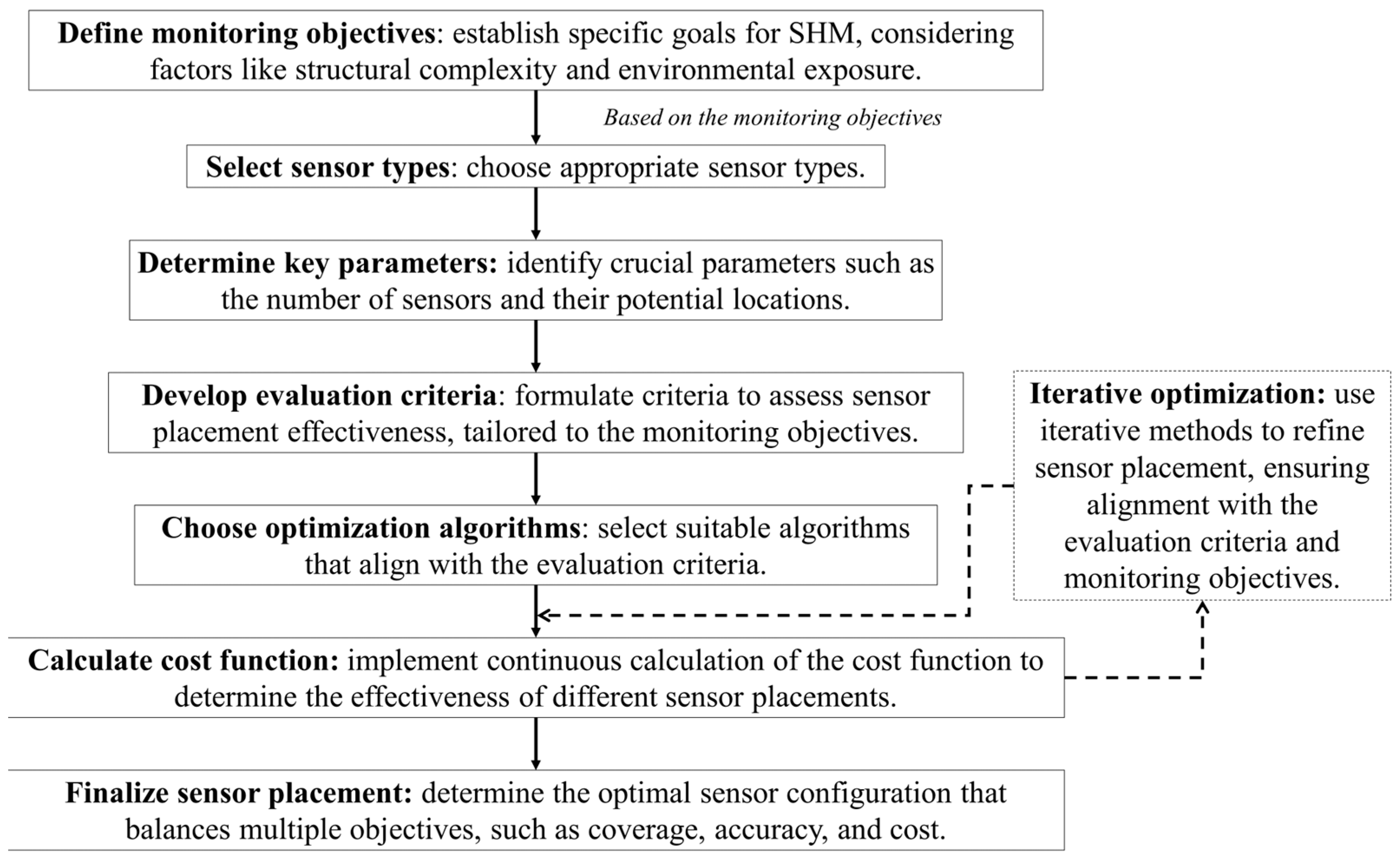
• Determining monitoring objectives according to the structural application.
• Determining the type of sensor which is suitable according to the monitoring objective.
• Determining parameters such as the number of sensors and the candidate locations of sensors.
• Determining evaluation criteria for the optimal placement of sensors.
• Determining the optimization algorithm for the optimal arrangement of sensors.
• Determining the cost function and the input parameters for the optimization algorithm.
• Determining the optimal solution for the sensor placement employing numerous calculations.

Within the steps involved, the pivotal points in OSP research are the evaluation criterion and the optimization algorithm. The evaluation criterion hinges on the specific monitoring objectives and must adeptly mirror the effectiveness of the sensor placement solution within those objectives. Typically, in the context of OSP, a continuous calculation of the cost function is imperative for ascertaining the optimal solution. Consequently, the structure and format of the evaluation criterion wield a substantial influence on the computational efficiency of the OSP, bearing substantial importance in this regard.

Optimization algorithms closely align with the chosen evaluation criteria, with the prevailing approach involving iterative iterations [11,12,13,14,15,16,17,18,19,20,21,22,23,24,25,26,27,28,29,30,31,32,33,34,35,36,37,38,39,40] to derive an OSP solution. In parallel, certain researchers have ventured into innovative territories, such as integrating neural networks into the process [41,42], to address this challenge, and this will be demonstrated later in this work.

Expanding upon these advancements, this paper further explores the practical implementation of OSP in real-world engineering scenarios. Emphasizing its diverse applications, OSP has proven integral in enhancing the safety and performance of various infrastructures. This is exemplified through successful case studies in monitoring Yingwuzhou Yangtze River Bridge, Canton Tower, and other key structures such as Shenzhen Sports Center, employing advanced OSP techniques. These real-life applications not only demonstrate OSP’s effectiveness but also its potential for future innovations in SHM.

Addressing practical needs, our study extensively reviews the existing literature in the OSP field, incorporating more than 200 relevant papers from major publishers such as Elsevier, Wiley, Springer, SAGE, and MDPI. This work aims to provide a comprehensive exploration of OSP within the SHM context, as depicted in Figure 1, offering detailed insights into evaluation criteria and optimization algorithms in OSP (Section 2 and Section 3), delving into current OSP strategies in the engineering sector (Section 4), and summarizing the challenges in current practices along with future trends in sensor placement (Section 5). Lastly, in Section 6, we synthesize and encapsulate the study’s main findings, with the integration of detailed analyses and real-world applications underscoring the paper’s significance in advancing OSP methodologies for SHM. Our work aims to serve as a bridge between theoretical research and engineering practice, providing both critical insights of the current OSP practice and the future research directions.

2. Evaluation Criteria

Before delving into the discussion of the evaluation criteria, it is necessary to understand that the various evaluation criteria currently developed are based on the monitoring objectives of SHM systems. Each evaluation criterion is imbued with a distinct perspective, thereby engendering scenarios where a sensor layout scheme may excel under specific criteria but falter under others. The pursuit of an equilibrium among all evaluation criteria simultaneously invariably leads to suboptimal results across the entire evaluation criteria, underscoring the need for deliberate compromises. In the process of selecting or formulating evaluation criteria, a judicious contemplation of the SHM system’s monitoring objectives is indispensable, underlining the significance of determining the specific facets and physical parameters deserving emphasis.

2.1. Maximum Vibration Signal

In the measurement of the actual engineering, the results will inevitably be contaminated by noise and other factors that make the measurement error, so the sensor can be placed by selecting the location of higher vibration amplitude, thus improving the signal-to-noise ratio effectively and ensuring the accuracy of the modal identification.

2.1.1. Modal Kinetic Energy (MKE)

To improve the signal-to-noise ratio of the collected data, Salama et al. [43] proposed to place sensors at measurement points where the structure has a large kinetic energy, which can increase the signal strength with relatively constant noise to improve the signal-to-noise ratio, that is, the modal kinetic energy (MKE) criterion, as shown in Equation (2).

$$MK{E}_i={\displaystyle {\sum }_{j=1}^{N_m}({\mathsf{\Phi }}_{ij}{\displaystyle {\sum }_k{M}_{ik}{\mathsf{\Phi }}_{kj}})}$$

(2)

In the equation, $N_m$ denotes the number of modal orders of the vibration modes involved in the calculation, ${\mathsf{\Phi }}_{ij}$ represents the $i^{th}$ row and $j^{th}$ column of the modal vibration matrix, and $M_{ik}$ represents the $i^{th}$ row and $k^{th}$ column of the overall mass matrix of the structure.

Parallel to the MKE approach, Stubbs et al. [44,45] introduced the modal strain energy (MSE) method. This method diverges by replacing the structural mass matrix with the structural stiffness matrix. The MSE method is considered a potent indicator for detecting structural damage. He et al. [46] put forth a sensor arrangement strategy. This approach harnesses the MSE method for acquiring the initial sensor arrangement, followed by the application of the modal assurance criterion (MAC) method to fine-tune and optimize the sensor placement, enhancing the overall effectiveness of the methodology.

2.1.2. Mode Shape Summation Plot (MSSP)

Similar to the MKE, the mode shape summation plot (MSSP) [47,48] also aims to improve the signal-to-noise ratio of the collected data by calculating the sum of the individual variables of the row vectors of the modal matrix to evaluate the performance of the corresponding sensor placement, as shown in Equation (3).

$$MSS{P}_i={\displaystyle {\sum }_{j=1}^{N_m}\left|{\mathsf{\Phi }}_{ik}\right|}$$

(3)

In Equation (3), $N_m$ denotes the number of modal orders of the vibration modes involved in the calculation, and ${\mathsf{\Phi }}_{ij}$ is the $i^{th}$ row and $j^{th}$ column of the modal vibration matrix. The ${MSSP}_i$ represents the modal component summing index of the $i^{th}$ degree of freedom of the structure, which is obtained by summing the absolute values of the modal amplitudes of the $N_m$ order of the $i^{th}$ degree of freedom. Based on the size of the ${MSSP}_i$ at each node, the degree of freedom with the largest ${MSSP}_i$ is selected as the sensor location.

Gui et al. [49] proposed a method for optimal sensor placement based on the mode shape summation plot (MSSP) and difference method (DM) with a modal confidence criterion test. They took the main girder of a railroad tie arch bridge as an example and compared the optimal sensor placement with the MSSP method, MSSP/DM method, and effective independence method, respectively, and examined the validity of the MSSP/DM method.

2.1.3. Eigenvector Component Product (ECP)

In Equation (4), $N_m$ denotes the number of modal orders of the vibration modes involved in the calculation, and ${\mathsf{\Phi }}_{ik}$ is the $i^{th}$ row and $k^{th}$ column of the modal vibration matrix. Similar to the MSSP method, the eigenvector component product [50,51] (ECP) involves simply taking the product of the eigenvector elements for a given candidate location across all modes of interest, where $i$ is the candidate sensor location and ${\mathsf{\Phi }}_{ij}$ is the $i^{th}$ element of the $j^{th}$ mode shape, $j$ is the order of the modal vibration shape, and $N_m$ is the maximum order of the modal vibration shape involved in the calculation. A maximum for this product is deemed to be a candidate measurement location.

$$EC{P}_i={\displaystyle {\prod }_{j=1}^{N_m}\left|{\mathsf{\Phi }}_{ij}\right|}$$

(4)

2.1.4. Driving Point Residue (DPR)

Imamovic [52,53] proposed the driving point residue (DPR) method based on the excitable degree of nodes for OSP, as shown in Equation (5).

$$DPR=\mathsf{\Phi }\otimes \mathsf{\Phi }{\Lambda }^{-1}$$

(5)

In Equation (5), Φ is the modal vibration matrix and Λ is the eigenvalue matrix of the structure. Larger DPR values indicate that the measurement points are more likely to be excited and therefore also to obtain a larger structural response, which leads to a higher signal-to-noise ratio. The later researchers [54] combined the DPR method with the effective independence method to overcome the drawback that the effective independence method tends to be selected at candidate points with low vibration intensity. Kaveh et al. [41] developed an efficient strategy based on the triaxial driving point residue (DPR3) coefficient and investigated it for large-scale dome-shaped trusses.

2.2. Maximum Modal Identification

A limited number of sensors cannot acquire all the modal information of a structure that needs to be acquired, so sensor placement can be optimized so that as much modal information as possible can be acquired.

2.2.1. Modal Assurance Criterion (MAC)

In structural dynamic testing, the aim is to ensure that the structural modal vectors are as distinct and independent from one another as possible. This independence is crucial for effectively identifying the modes of vibration. Carne and Dohmann [55] introduced the modal assurance criterion (MAC), which utilizes the independence of the vectors recorded by sensors as a means to facilitate a more straightforward distinction of the modal vibration patterns.

$$MACij=\frac{{({\mathsf{\Phi }}_i^T{\mathsf{\Phi }}_j)}^2}{({\mathsf{\Phi }}_i^T{\mathsf{\Phi }}_i)({\mathsf{\Phi }}_j^T{\mathsf{\Phi }}_j)}$$

(6)

In Equation (6), ${MAC}_{ij}$ denotes the variable in $i^{th}$ row and $j^{th}$ column of the MAC matrix, respectively; where $\mathsf{\Phi }$ is the mode shape matrix and subscripts i and j refer to the $i^{th}$ and the $j^{th}$ column vectors. The MAC matrix’s non-diagonal elements show the correlations between the modal vibration vectors of various orders, whereas the diagonal elements consistently hold a value of 1. The non-diagonal elements have values between 0 and 1. A value approaching 1 signifies a strong correlation between the respective modal vibration vectors, while a value closer to 0 indicates a diminished correlation. Carne and Dohmann suggested that for effective mode distinction, the maximum value of the non-diagonal elements within the MAC matrix should not exceed 0.25. This criterion serves as a reliable guideline in assessing the independence and discriminability of the modal vibration patterns, ensuring that the identified modes are delineated.

The MAC has established itself as a versatile tool with a wide array of applications, garnering extensive attention and development from researchers. One notable extension of the MAC was undertaken by Yi et al. [25], who advanced the criterion to encompass three-directional sensors. This involved a thoughtful exploration of various placement strategies for both unidirectional and three-directional sensors, culminating in the introduction of the three-dimensional MAC. In another context, An et al. [56] studied the optimal number and placement of sensors in vibration-based damage detection of composite materials, treating the number and location of sensors as design variables, while material properties, ply thickness, and ply orientation angles were considered random variables. Notably, they assessed the effectiveness of sensor placement by employing the root-mean-square error of the MAC matrix, providing valuable insights into optimizing sensor arrangements for damage detection in composite materials.

2.2.2. Redundancy of Mode Shape (RMS)

Addressing the spatial continuity of modal vibration patterns reveals that identical or symmetrical sensor placements tend to capture similar or symmetrical modal vibration data. Such repetitive modal information, while abundant, does not substantially contribute to the structural analysis and should be minimized. This concept has been coined the “Redundancy of Mode Shape” (RMS) criterion, as named by Stephan [57], and is represented by Equation (7). This criterion plays a significant role in OSP by emphasizing the avoidance of redundant modal information.

$$R_{ij}=1-\frac{{\Vert {\mathsf{\Phi }}_i-{\mathsf{\Phi }}_j\Vert }_F}{{\Vert {\mathsf{\Phi }}_i\Vert }_F+{\Vert {\mathsf{\Phi }}_j\Vert }_F}$$

(7)

In the equation, ${\mathsf{\Phi }}_i$ and ${\mathsf{\Phi }}_j$ denote the modal vibration row vectors corresponding to the $i^{th}$ and $j^{th}$ degrees of freedom, respectively. When the value of $R_{ij}$ is larger, it means that the information measured by the $i^{th}$ and $j^{th}$ sensors is nearly the same and one of them can be discarded.

Lin et al. [58] proposed a multi-objective optimization algorithm, which is based on the particle swarm algorithm and considers three objective functions: linearly independent mode shapes, dynamic information redundancy, and vibration response signal strength. This is applied to a simplified finite element beam model of a target building and compared with other selection methods, and the results show that the algorithm balances the objective functions reasonably well and outperforms the other methods. Yi et al. [25] proposed a method for triaxial acceleration sensors, which was established by combining a tridimensional modal assurance criterion and the redundancy function and solved by using the hierarchical wolf algorithm, and the proposed method was validated by a benchmark bridge model. The results show that the method can ensure the optimal configuration of the triaxial sensors.

2.2.3. Singular Value Decomposition Ratio (SVDR)

In 1996, Golub and Loan introduced a valuable sensor optimization criterion known as the singular value decomposition ratio (SVDR), relying on the singular values of the modal matrix [59]. The SVDR serves as a direct gauge of the orthogonality and observability of modal vibrations, bearing substantial physical significance in the context of optimization parameters, as depicted in Equation (8). This criterion plays a pivotal role in enhancing sensor placement strategies for SHM.

$$SVDR=\frac{{\sigma }_{\max }}{{\sigma }_{\min }}$$

(8)

In Equation (8), ${\sigma }_{max}$ and ${\sigma }_{min}$ are the maximum and minimum singular values of the modal vibration matrix, respectively. When the value of SVDR is smaller, it indicates that the vectors tend to be more orthogonal, and when the lower limit of SVDR of 1 is reached, it indicates complete orthogonality.

Cherng et al. [60], based on the signal subspace correlation technique which they developed, performed a singular value decomposition of the Hankel matrix consisting of the candidate positions of the sensors to obtain the optimal sensor placement. Chhabra et al. [61] applied a modified control matrix and singular value decomposition (MCSVD) method to optimize the placement of piezoelectric actuators on a thin plate and obtained the optimal placement of the actuators by maximizing the MCSVD using the modified heuristic genetic algorithm.

2.3. Minimum Parameter Identification Error

In the identification of structural parameters, due to the influence of measurement noise and other factors causing the error between the results of parameter identification and the true results, it is possible to optimize the placement of the sensors to increase the amount of information acquired, reducing the uncertainty of parameter identification.

2.3.1. Fisher Information Matrix (FIM)

Kammer [62] proposed the Fisher information matrix (FIM) concept to ensure the linear independence of the vectors measured by the sensor and to reduce the uncertainty of the measured information, as shown in Equation (9):

$$FIM={\mathsf{\Phi }}_S^T{\mathsf{\Phi }}_S$$

(9)

Within the equation, ${\mathsf{\Phi }}_s$ denotes the measurement vector matrix composed of sensors. In the context of OSP, the emphasis lies on the minimization of the covariance matrix pertaining to estimated parameters. This is achieved through the maximization of the determinant and trace of the measurement vector matrix, or the minimization of singular values. These optimization strategies serve to enhance the quantity of estimated information or to diminish the associated uncertainties in the estimated parameters.

Diverse research efforts have significantly contributed to the realm of sensor arrangement optimization in SHM and modal identification. Bayard et al. [63] proposed a method that decouples measurement point arrangement from input parameter design, maximizing the determinant of FIM for OSP in large structures. Borguet et al. [64] used a weighted summation of parameters, including determinants and traces of the FIM, for OSP. Yang et al. [24] proposed a robust OSP method for SHM considering uncertainty, based on interval analysis method and modal analysis, and derived the interval FIM from the deterministic case, where the determinant is considered as an optimization function. Yi et al. [25] proposed a form of a three-dimensional FIM for three-axis acceleration sensors. Loutas et al. [16] addressed redundant sensor placement concerns and developed an optimal placement technique for modal recognition and vibration-based SHM. An et al. [65] proposed a robust framework for the OSP problem under sensor clustering considering both sensor faults and vibration-based damage detection, replacing the original FIM with the sum of the mean and standard deviation of the minimum determinant.

2.3.2. Information Entropy (IE)

Papadimitriou et al. [66] introduced the concept of information entropy (IE) into the Bayesian model update theory, using information entropy to quantify the uncertainty in the identification of structural stiffness parameters and selecting the OSP by minimizing the value of IE, as shown in Equation (10).

$$H(D)=E_{\theta }[-\ln p(\theta |D)]=-{\displaystyle \int p(\theta |D)}\ln p(\theta |D)d\theta$$

(10)

$$p(\theta |D)=c{[J(\theta ;D)]}^{-\frac{N{N}_0-1}{2}}{\pi }_{\theta }(\theta )$$

(11)

$E_{\theta }$ is the mathematical expectation of $\theta$, $\theta$ is the modulus of the structural parameter to be identified, and $D$ is the test data obtained by the sensor. $p\left(\theta |D\right)$ can be calculated according to Equation (11), where $J(\theta ;D)$ is the degree of fit of the measured data to the model response time, $N$ is the number of sampled data, and $N_0$ is the number of observed degrees of freedom of the structural model. From Equation (11), the IE is the negative logarithm of the expectation of the posterior probability density function. When the value of IE is smaller, it means that the uncertainty of parameter identification is smaller.

In subsequent studies, several researchers have made significant contributions to the domain of sensor optimization for various applications within SHM. Papadimitriou et al. [67,68] introduced Laplace asymptotic integration to simplify the computational process. Yang et al. [69] integrated Bayesian risk into sensor optimization, aiming to minimize the expected loss of the decision outcome. Colombo et al. [29] presented a framework for SHM sensor network design, defining the fitness function in terms of Bayesian risk, to maximize detection probability while minimizing the overall cost.

Yuen et al. [30] introduced robust IE to quantify model parameter uncertainty, considering sensor faults and enhancing robustness in the designed configurations. Bansal et al. [70] proposed an optimal Bayesian sensor layout method that employs a two-stage update process with environmental vibration data for model updating, selecting the sensor configuration that maximizes information gain in model parameters. Pei et al. [71] introduced a conditional IE-based sensor layout method to examine the impact of measurement noise and model error on sensor placement separately, representing model error using variations in the cell stiffness matrix.

Bertola et al. [20] investigated a measurement system design method for dynamic testing, utilizing desired information on self-oscillation frequency. They employed modal-frequency joint IE for sensor arrangement optimization. Mehrjoo et al. [72] introduced an information-theoretic-based OSP layout framework for parameter estimation, virtual sensing, and state monitoring. This framework incorporated Bayesian OSP approaches and modal expansion to minimize the IE of quantities of interest. It achieved this without prior knowledge of the input excitation. Underpinning these works is the concept of IE, which quantifies the uncertainty or unpredictability in a system. In sensor networks and Bayesian decision making, entropy is indicative of the reliability of sensor data and the ensuing predictions. High entropy suggests greater uncertainty, influencing Bayesian risk and the associated decision-making processes.

2.3.3. Mutual Information (MI)

To promote the independence of vectors acquired through sensor measurements, a valuable approach is to analyze the information gathered by these sensors. When the information obtained from distinct sensors exhibit lower interconnections, it signifies a tendency towards greater independence among the vectors they capture. Mutual information (MI) [73] serves as a valuable metric for quantifying the interdependence between different variables, as expressed in Equation (12).

$$I(x,y)={\log }_2[\frac{p_{X,Y}(x,y)}{p_X(x)p_Y(y)}],$$

(12)

where $x,y$ are the measured values at points $X,Y$, respectively, $p_X\left(x\right)$ and $p_Y\left(y\right)$ are the marginal probability density functions of $X,Y$, respectively, and $p_{X,Y}(x,y)$ is the joint probability density function of $x,y$.

MI measures the degree of information overlap between two sensors, indicating redundancy in their measurements. OSP involves minimizing MI between sensor data and enhancing system efficiency. Mark et al. [74] introduced an approach using MI as an evaluation criterion to select sensor locations for maximizing information about structural damage parameters. Bhattacharyya et al. [75] computed MI between predicted sensor data and system model parameters and transformed it into a relaxed convex optimization problem, evaluating informativeness and optimal solutions efficiently. These approaches ascertained both the informativeness of the problem and the potential optimal solutions in an efficient and structured manner.

2.4. Data Reconstruction Error Minimization

In the context of monitoring random vibration structures, scenarios occasionally arise where certain critical locations are unable to accommodate measurement points, or the number of available sensors falls short of covering these critical points. In such cases, mathematical techniques like Kalman filtering [76], system equivalent reduction expansion process [77,78], Guyan static reduction/expansion [79], and others can be applied to compute data for unplaced sensor locations based on information collected from existing sensors. The accuracy of the reconstructed data is significantly influenced by the arrangement of sensors, prompting the pursuit of an OSP to minimize errors in the reconstructed data. For instance, to achieve the minimization of variance in the reconstructed response, as depicted in Equation (13).

$$\Delta =\mathrm{cov}(y_k-y_k^e)$$

(13)

In Equation (13), $y_k$ is the true value of the response location and $y_k^e$ is the value of the response location calculated using mathematical means. The optimal placement of the sensors is obtained by minimizing the response variance.

Significant advancements have been achieved by researchers in enhancing the utilization of the minimization method within the realm of SHM. These contributions encompass various key facets, such as the reduction in error variance [11] for heightened precision, as well as the enhancement of damage detection [80] and early damage sensing [81]. Furthermore, researchers have directed their attention to the refinement of sensors, addressing factors including sensor normal distance [82] and apparatus configuration [33]. It is worth noting that the Kalman filter has emerged as an invaluable tool in assessing the effectiveness of sensor placement [83] and facilitating the seamless fusion of data [84]. Collectively, these research efforts significantly elevate the sophistication and applicability of SHM methodologies.

2.5. Probability-Based Damage Detection

The fundamental objective of SHM systems is to acquire dynamic parameters of a structure to effectively assess its operational state, with a particular emphasis on damage detection. In this context, Flynn and Todd [85] introduced a global optimality criterion for addressing the challenge of damage detection within a Bayesian risk minimization framework. This framework is designed to optimize the allocation of sensing network resources, with the overarching goal of minimizing the expected occurrence of Type I or Type II errors; Equations (14) and (15) elucidate these critical concepts within the context of SHM damage detection.

$${\overline{P}}_{FA}={\displaystyle {\sum }_{k=1}^K\frac{P(d_{k1}|h_{k0})P(h_{k0})}{{\displaystyle {\sum }_{k=1}^{K}P(h_{k0})}}}$$

(14)

$${\overline{P}}_D={\displaystyle {\sum }_{k=1}^K\frac{P(d_{k1}|h_{k1})P(h_{k0})}{{\displaystyle {\sum }_{k=1}^{K}P(h_{k1})}}}$$

(15)

In the above equation, ${\overline{P}}_{FA}$ represents the global false alarm rate, which is the expected proportion of undamaged regions of the structure that are incorrectly identified as damaged or presenting Type I errors. ${\overline{P}}_D$ stands for the global detection rate, a key performance metric that signifies the expected proportion of damaged regions correctly identified as such. $P\left(d_{k1}|h_{k0}\right)=\mathrm{P}\mathrm{r}\left(T\right[k]>\mathsf{\gamma }[k\left]h_{k0}\right)$ is the local detection rate of region $k$. $h_{kj}$ represents the actual local damage state ($j=0$ means undamaged, $j=1$ means damaged). $P\left(h_{kj}\right)$ represents the prior probability of the local damage state. $d_{kj}$ is the event that determines $h_{kj}$ as the local damage state in region $k$.

Furthermore, an extensive body of research has yielded various methodologies aimed at OSP for effective damage detection. Ručevskis et al. [86] delved into the problem of OSP for damage identification in composite structures. Hou et al. [87] employed sparse recovery theory to address structural damage detection by integrating a meta-heuristic algorithm for OSP. This approach focused on minimizing the mutual coherence of the sensitivity matrix within L1-regularized damage detection. Notably, the method leveraged the sensitivity matrix from the undamaged state, eliminating the need for prior knowledge of damage location and severity.

In a complementary effort, Downey et al. [23] introduced a sensor multi-objective optimization algorithm. This algorithm was developed to mitigate the occurrence of Type I and Type II errors in SHM systems by utilizing the system error with the estimated response and IE as bi-objective optimization criteria. These research contributions collectively enhance the capabilities of damage detection in structural systems through sophisticated sensor placement strategies.

2.6. Minimum Energy Consumption

Large structures, owing to their intricate designs and diverse features, often present challenges for the deployment of wired sensors, primarily related to layout constraints and connectivity issues. In contrast, wireless sensors offer a distinct advantage as they obviate the need for cumbersome communication cables, simplifying both arrangement and installation processes. However, the energy supply for wireless sensors remains a critical concern, and the distance between sensors and base stations directly impacts energy consumption, underscoring the significance of OSP to extend the operational lifespan of wireless sensors. Notably, Zhou et al. [88] introduced a comprehensive theoretical framework for addressing the optimal placement of wireless sensors, focusing on the attainment of an optimal configuration that enhances recognition quality and network performance. This research contributes significantly to the enhancement of wireless sensor deployment strategies in the context of large structures.

$$EC=f(EC{E}_u,EC{P}_w)(u=1,2,\dots ,N_E;w=1,2,\dots ,N_p)$$

(16)

$$ECE=f(M,K,C,D,L_0,\varsigma )$$

(17)

$$ECP=f(SP,SE,SL,RP,SR,NR,FD,NC,\xi )$$

(18)

$EC$ represents the evaluation criterion, $ECE$ represents the structural performance evaluation criterion, and $ECP$ represents the wireless sensor network performance evaluation criterion. $M$, $K$, and $C$ represent the mass matrix, stiffness matrix, and damping matrix of the structure, respectively, $\varsigma$ is the measurement error, $L_0$ is the observation matrix, and $D$ is the sensor sampling data. $SP$ is the sensor location, $SE$ is the sensor energy, $SL$ is the sensor load, $RP$ is the sensor communication protocol, $SR$ is the sensor stability, $NR$ is the sensor network robustness, $FD$ is the detectability of network failure, $NC$ is the network cost, and $\xi$ is the influence of environmental factors. Zhou et al. [88] achieved the linear independence of the identified modal vibrations by the above equations, ensuring the connectivity of the wireless sensor network and pursuing the energy efficiency of the whole wireless sensor network.

Numerous studies have delved into OSP within wireless sensor networks, addressing crucial facets such as energy consumption, information transmission, and network efficiency. Notably, some research has focused on algorithmic approaches [89] to balance information quality and energy efficiency in sensor placement. Others have concentrated on rechargeable sensor placement, specifically tackling the minimum permanent coverage node placement problem [90]. Additionally, strategies for optimizing relay node placement, considering energy conservation and monitoring efficiency, have been explored in separate studies [91,92]. The utilization of split clusters within sensor networks has shown promise for SHM [93]. Moreover, comprehensive network optimization, with an emphasis on minimizing energy consumption, incorporates power control, packet transmission with error-correcting codes, and topology control [94,95]. Furthermore, integrated efforts encompass aspects like sensor locations, activity schedules, reference sensor movement trajectories, and data stream transmission routes [40].

2.7. Others

2.7.1. Cost

An often overlooked yet simple aspect is the actual cost involved in OSP. The cost is influenced by the location of the sensors. For instance, in the scenario depicted in Figure 2, where all properties require SHM, the cost at location B could be higher than at locations A and C due to its position in the middle of a water body. Researchers sometimes may need to consider such finical effects in the overall optimization progress [96].

2.7.2. Coverage

Previously, optimization criteria viewed sensors collectively, but focusing on each sensor individually reveals that coverage is crucial [97], especially for the wireless sensors that need to consider the effectiveness of data transmission [98,99]. Wu et al. [100] delve into this aspect for indoor environments, specifically addressing the critical-grid coverage problem, as shown in Figure 3. This paper proposes a multi-objective optimization model considering both accuracy and cost, employing the NSGA-II algorithm for optimization to achieve OSP and demonstrates the practical effectiveness of the proposed method.

Geometry significantly influences sensor coverage in SHM, particularly for vision-based sensors. As shown in Figure 4, sensors at higher elevations typically offer wider coverage, while those at lower levels may face coverage limitations due to obstructions or viewing angles. Additionally, the orientation and angle of the sensors need to be strategically aligned with the structure’s geometry to avoid blind spots and ensure comprehensive monitoring. Environmental conditions like lighting and weather also play a role in affecting sensor performance. Proper placement considering these factors is essential for effective and reliable SHM.

2.8. Summary of the Section

Several noteworthy studies have contributed diverse perspectives to the realm of OSP. Thiene et al. [102] delved into damage identification via guided waves, considering various evaluation criteria such as information independence, Lamb wave characteristics, boundary reflections, attenuation profiles, excitation amplitudes, and geometric complexities. Zhang et al. [35] introduced an innovative framework for SHM that amalgamates OSP rooted in finite element modal analysis with an evidence inference criterion, leveraging probabilistic and fuzzy uncertainty handling. In the domain of uncertain inverse problems for structural parameter estimation, Liu et al. [103] proposed the maximum independent mean-variance criterion to guide OSP. Sadhu et al. [104] employed blind source separation and tensor decomposition for modal identification, utilizing the resultant modal parameters to formulate an optimization function for sensor placement. Biswal et al. [105] proposed a Markov chain Monte Carlo algorithm based on distance measurements for determining the optimal placement of the accelerometer and the impact hammer. Shi et al. [106] proposed a weighted standard deviation norm index-based approach, focusing on the significance of damage in structural performance, while Yang et al. [28] explored uncertain load-dependent sensor placement by leveraging non-probabilistic response reconstruction theory. Ghosh et al. [107] established a method for OSP under basal excitation, emphasizing a stochastic input–output relationship in the frequency domain and modeling seismic input as a nonstationary stochastic process with uniform modulation. These contributions collectively enrich the field of sensor optimization for SHM.

In general, the MAC is the most widely used criterion for sensor placement in SHM. It is simple to understand, calculate, and interpret. However, it is important to note that the MAC does not consider the uncertainty in the modal identification process. The FIM can be used to overcome this limitation, but it can be computationally expensive, especially for large structures. The MKE, MSSP, and ECP criteria are all simple to calculate and interpret, and they are not sensitive to sensor placement errors. However, they do not consider the uncertainty in the modal identification process. Rather than evaluating each criterion individually, the previously mentioned criteria are organized into six distinct groups. A comparison of these groups is presented in

Table 1. Summary of the evaluation criterion involved.

Criterion	Description	Advantages	Disadvantages
Maximum Vibration Signal	Emphasis on high-intensity vibration signal acquisition.	Enhances signal clarity, pivotal for detecting significant structural changes.	Risk of neglecting subtle, yet crucial, structural signals.
Maximum Modal Identification	Optimization towards comprehensive modal information capture.	Facilitates in-depth analysis of structural dynamics.	Involves high computational resource allocation and complexity.
Minimum Parameter Identification Error	Precise estimation of structural parameters.	Increases reliability and accuracy in structural assessments.	Necessitates advanced computational algorithms, elevating operational intricacy.
Data Reconstruction Error Minimization	Aimed at high fidelity in data interpretation and reconstruction.	Ensures integrity and reliability of the data reconstruction process.	Computationally demanding, requiring sophisticated data handling capabilities.
Probability-Based Damage Detection	Utilizes probabilistic methods for early structural damage detection.	Facilitates early intervention and nuanced understanding of damage probabilities.	May yield non-definitive results due to inherent probabilistic nature.
Minimum Energy Consumption	Focus on energy-efficient sensor placement and functioning.	Promotes sustainable and cost-effective monitoring, especially long term.	Could limit data collection scope in energy-constrained setups.

.

It is important to note that the choice of the most appropriate criterion for sensor placement in SHM is highly contingent on the specific objectives of the application at hand. If the primary aim is to minimize uncertainties within the modal identification process, the FIM stands as the optimal selection. However, scenarios, where the emphasis is on streamlining sensor placement procedures or curtailing computational expenses, necessitate alternative criteria, such as the MAC, MKE, MSSP, or ECP, which may yield more favorable outcomes.

In short conclusion, OSP in SHM is a multifaceted and complex process that goes beyond just adhering to physical criteria such as cost and coverage for the sensors, requiring a thorough and strategic approach, as summarized in Figure 5. The practicalities involved are multifarious, encompassing budgetary limitations, sensor availability, structural considerations for sensor installation, as well as the environmental factors at hand. These elements collectively highlight the nuanced and multifaceted nature of sensor placement within SHM. Such considerations must coalesce to inform an optimal strategy that effectively meets the monitoring objectives. Hence, a thorough and detailed evaluation of the application’s unique demands and limitations is paramount. This ensures that the chosen sensor placement strategy is not only theoretically sound but also practically viable, aligning with both the objectives and the tangible conditions of the SHM project.

3. Optimization Methods

OSP methods can be roughly divided into deterministic and stochastic algorithms; if we can simplify the OSP problem into a continuous function to find the extremum, deterministic algorithms can be used to obtain the OSP solution easily. However, for most of the problems, the structure is complex and the candidate positions of the sensors are discrete. It is impossible to transform them into a continuous function to find the extremum; therefore, the deterministic algorithms are not suitable for real-world problems [9]. For such combinatorial optimization NP-hard problems, meta-heuristic algorithms can find acceptable results efficiently. This section presents detailed information about different types of optimization methods.

3.1. Deterministic Sensor Placement Algorithm

In the realm of SHM, the application of deterministic optimization methods for sensor placement in relatively simple beam and plate structures has proven effective. These methods encompass both constrained, such as linear and nonlinear programming [108], and unconstrained optimization techniques, like Newton’s method [109]. However, these deterministic methods inherently rely on continuous variables, which means they are most suited for structures with continuous variable candidate sensor locations, as typically found in simple planar structures. The complexity of large-scale structures necessitates discrete sensor locations, posing a challenge for deterministic optimization. To bridge this gap, creative solutions have been explored. Sepulveda et al. [110] introduced an innovative approach that treats sensor placement as a mixed design problem, encompassing 0–1 continuous variables. This method extends the applicability of deterministic optimization to large structures by effectively transforming discrete sensor locations into continuous variables.

3.2. Sequential Sensor Placement Algorithm

The sequential sensor placement algorithm represents an iterative approach for systematically determining the placement of individual sensors through a series of successive computations, ultimately culminating in the arrangement of all sensors. This algorithm is conceptually categorized into two distinct strategies known as forward sequential sensor placement (FSSP) and backward sequential sensor placement (BSSP).

The FSSP method operates by identifying eligible sensor placement sites within the structural nodes. In a stepwise manner, it proceeds to place sensors at candidate locations that induce the most substantial improvements in the evaluation criterion. Subsequently, sensors are placed at the remaining candidate locations, and this process iterates until all sensors have been positioned optimally. A notable instantiation of this method is exemplified by the minimize modal assurance criterion (MinMAC) approach [55], pioneered by Carne and Dohrmann. Here, a set of candidate locations is empirically determined, and in each iteration, the candidate location that minimizes the non-diagonal elements of the MAC matrix is chosen as the sensor location, contributing to the establishment of the final sensor placement.

The BSSP assumes that all candidate points on the structure are arranged with sensors, and the sensor location that minimizes the change in the evaluation criterion is selected for deletion by continuous iterative computation until a predetermined number of sensors is reached. This method is represented by the effective independence (EI) [62] method, in which Kammer utilized the modal matrices of all candidate locations, calculated the FIM, ranked each candidate sensor location according to its contribution to the independence of the target modal matrix, and used an iterative method to sequentially remove the alternative sensor location with the smallest contribution in each iteration step.

The sequential sensor placement algorithm offers the advantage of computational simplicity, rendering it accessible for practical applications. Nevertheless, its primary drawback lies in its limited efficiency. This reduced efficiency results from the necessity to iterate through all candidate measurement locations to identify the optimal placement. Particularly, for large-scale structures featuring thousands of degrees of freedom, this computational process becomes notably protracted [111]. Furthermore, the interactions or conflicts that may arise between newly added or removed sensors and those previously selected contribute to the inherent limitation of achieving a globally optimal solution [112].

3.3. Meta-Heuristic Optimization Algorithm

As the sequential sensor placement algorithm encounters limitations when applied to large structures, extensive research efforts have been dedicated to the exploration and refinement of optimization algorithms. Notably, in the 1970s, John Holland [113] introduced the genetic algorithm (GA), a paradigm that garnered global recognition due to its versatility and swift problem-solving capabilities. This algorithm leverages computer-based simulations to emulate the biological evolutionary processes of gene crossover and mutation, transforming problem-solving into an evolutionary process. Numerous researchers have contributed refinements aimed at enhancing convergence speed and achieving global optima [114,115]. Alongside the GA, other optimization techniques such as particle swarm optimization (PSO) [116], ant colony algorithm [117], artificial bee colony algorithm [118], monkey swarm algorithm [119], firefly algorithm [120], and more have found application in sensor arrangement. In this paper, the methods employing GA and PSO will be introduced in more detail, serving as examples for OSP applications.

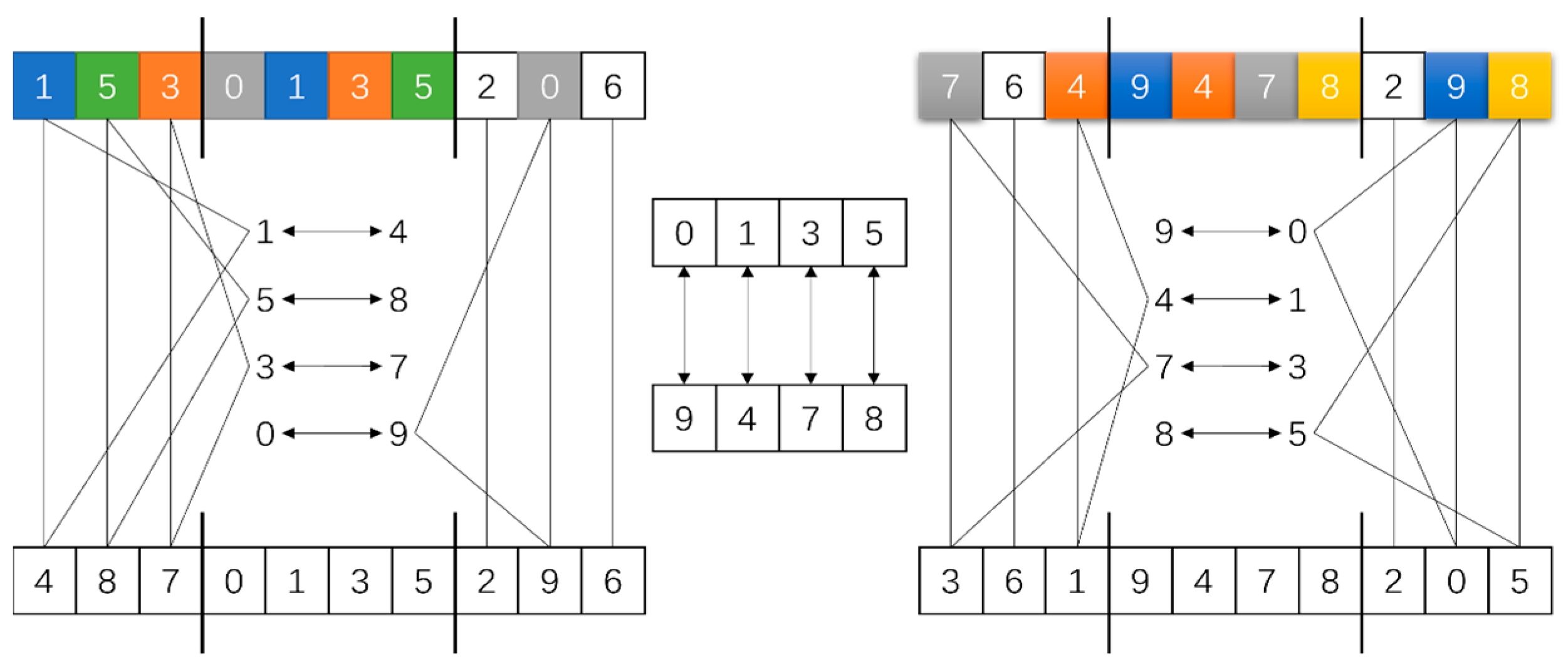
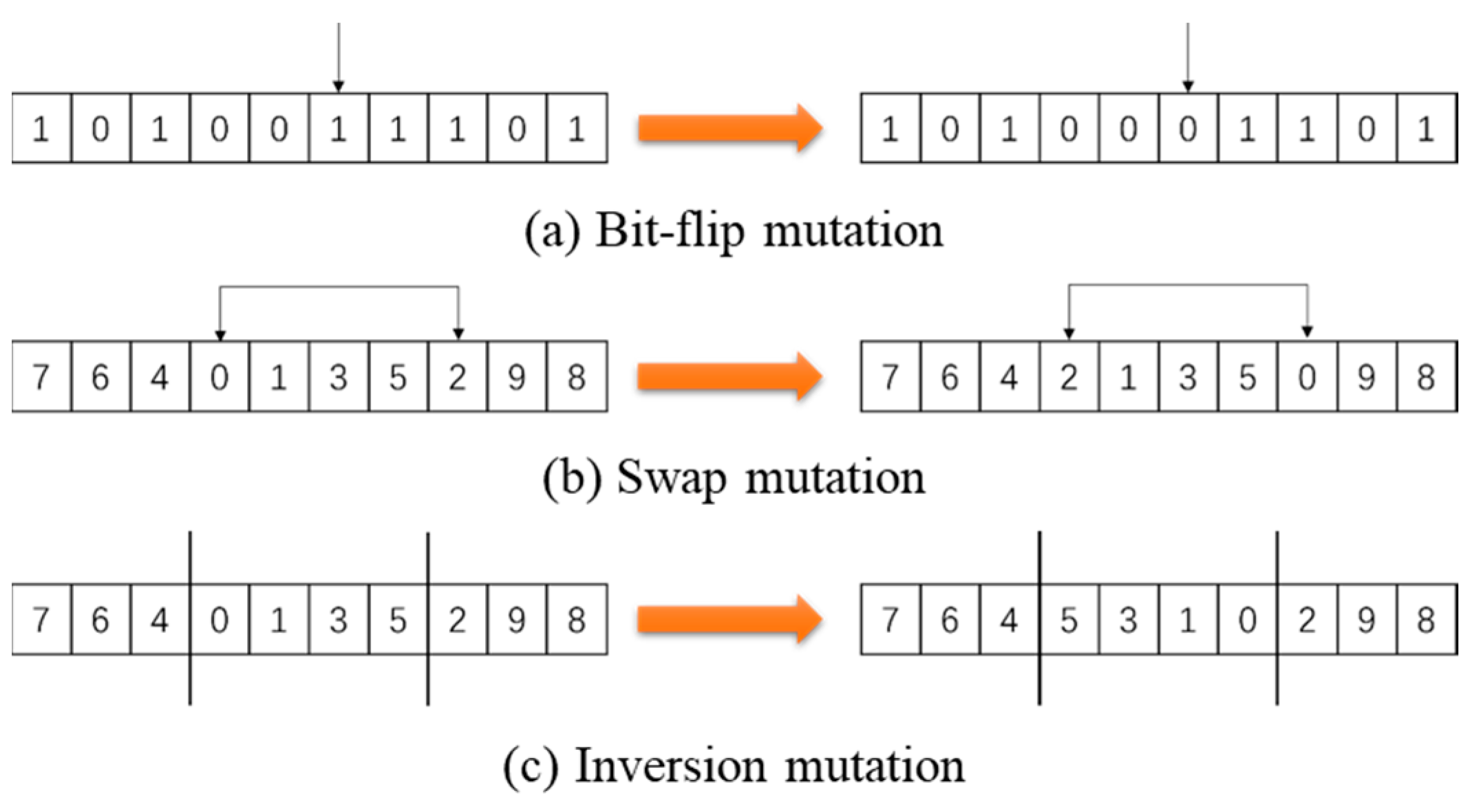
3.3.1. Genetic Algorithm (GA)

The GA operates through stages of initialization of chromosome sets, fitness evaluation based on predefined criteria, chromosome ranking and culling by fitness, and generation of new chromosomes via crossover and mutation [121], as demonstrated in Figure 6 and Figure 7, where ‘0’ and ‘1’ represented the absence or presence of sensors at specific locations. Due to challenges in this method during crossover and mutation [122], alternative encodings like integer [123], floating-point [124], decimal two-dimensional array [125], quantum probability vectors [126], and dual-structure coding [127] were developed to improve computational efficiency and stability in GA operations.

Following the initial generation and fitness evaluation, the GA then comes into a crucial selection phase, vital for their effectiveness and convergence [128]. Methods include roulette wheel selection, tournament selection, Boltzmann selection, and random universal sampling selection. Roulette wheel selection assigns each chromosome a section on a roulette wheel proportional to its fitness, choosing by random draw [129], while tournament selection pairs chromosomes randomly, selecting the fittest from each pair for further evolution [130]. These selection methods are pivotal in guiding the GA towards optimal convergence.

After chromosome selection, the GA perform crossover operations to generate new generations. Methods include single-point, double-point, K-point, uniform, and partially matched crossover. Single-point crossover involves exchange segments beyond a random point between two chromosome [131] (Figure 7a), while double-point crossover uses two crossover points (Figure 7b,c). However, these methods may produce duplicate or missing codes, leading to the use of variants like partially matched crossover, which replace duplicates in the non-swapped segment with elements from the swapped parent [132] (Figure 8). These techniques are essential for the evolution of chromosomes in GA, ensuring viable new generations.

Mutation operations in GA are crucial for maintaining genetic diversity and avoiding local optima. Techniques included bit-flip mutation, swap mutation, inversion mutation, and reverse mutation. Bit-flip mutation changes a specific bit from 0 to 1 or vice versa, as shown in Figure 9a. Swap mutation randomly exchanges values between two positions, as demonstrated in Figure 9b. Reverse mutation selects a chromosome segment and reverses the order of its elements [130], as depicted in Figure 9c. These methods introduce variability, helping GA explore the solution space more effectively and prevent settling on suboptimal solutions.

The effectiveness of GA in finding optimal solutions relies on their iterative nature factors like population size, search space dimensionality, and the number of iterations significantly impact their performance [133,134]. Reliable results often require multiple runs of the algorithm, with the best solution chosen from the outcomes. The ‘no free lunch’ theorem [135] highlights that no single algorithm excels across all problem, emphasizing the need for problem-specific algorithm selection or development.

Numerous researchers have enhanced GA for various applications. Nasr et al. [81] enhanced SHM using an optimization algorithm with ensemble Kalman filtering (EnKF), tested on a 10-story building. Liu et al. [136] focused on OSP for bridge structures using a single parents GA. Kang et al. [137] introduced a virus coevolutionary parthenogenetic algorithm (VEPGA), integrating a parthenogenetic algorithm with viral evolution theory for modal recognition in large spatial structures, exemplified by portal frames and concrete arc dams. Yi et al. [122] developed a generalized GA for the tallest building in northern China. Fiber-reinforced shell structures benefited from Nandy et al. [138], using an island model parallel GA to achieve enhanced computational efficiency. Ganesan et al. [139] proposed a GA using a 2D discrete Daubechies 4 (db4) lifting wavelet transform for sensor placement, and Kim et al. [140] introduced an Adam mutation genetic algorithm (AMGA) for pipeline monitoring.

Additionally, Qin et al. [141] proposed a parthenogenetic algorithm for optimizing sensor placement based on initial sensor distribution, verified with a terminal container crane case study. These advancements in GA demonstrate the algorithm’s adaptability and efficacy across diverse applications, underscoring the importance of selecting or developing algorithms tailored to specific project requirements.

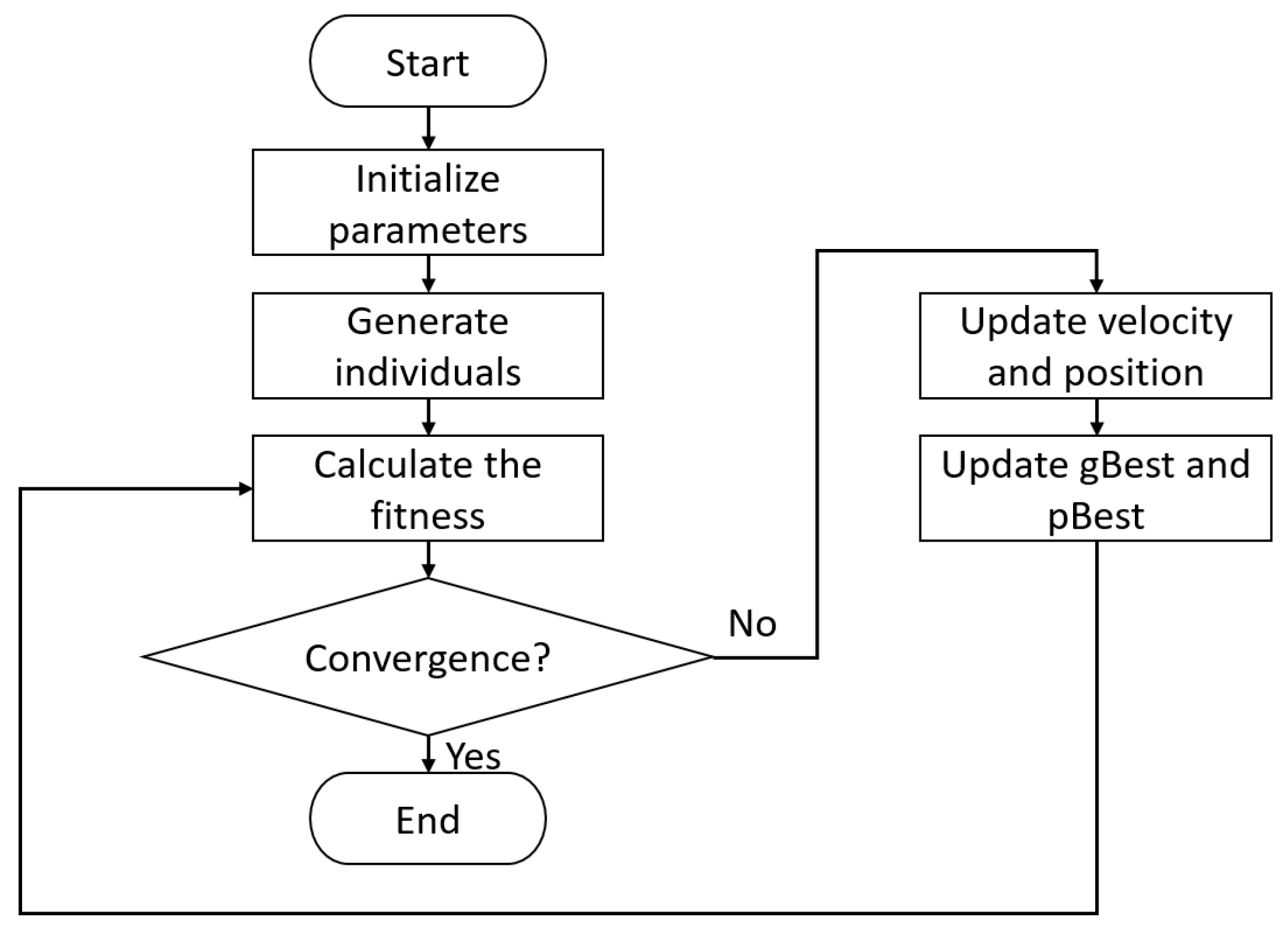
3.3.2. Particle Swarm Optimization (PSO)

The particle swarm optimization (PSO) algorithm, developed by Kennedy and Eberhart in 1995, is inspired by the foraging behavior of birds [142]. It simulates how birds adjust positions to find food, with each ‘particle’ representing a potential solution. The algorithm iterates as particles update their velocities and positions based on experiences, effectively converging on optimal solutions [143,144]. This method is influential in various fields, particularly in complex optimization scenarios.

In PSO, each particle possesses velocity and position attributes, essential for movement and direction. Particles independently search for their optimal solution, the ‘personal best’ (pbest), which is shared within the swarm. The most effective pbest becomes the ‘global best’ (gbest), symbolizing the swarm’s collective optimal solution at any point. Particles dynamically adjust speed and position, influenced by the interplay between their pbest and the swarm’s gbest [145]. This individual and collective refinement process is key to the algorithm’s success in complex environments.

The velocity and displacement of the particle are calculated as shown in the following equation [146]:

$$V_k(i+1)=\omega V_k(i)+c_1{r}_1(p_{best,i}^k-X_k(i))+c_2{r}_2(g_{best,i}-X_k(i))$$

(19)

$$X_k(i+1)=X_k(i)+V_k(i+1)$$

(20)

$$\omega ={\omega }_{\max }-\frac{{\omega }_{\max }-{\omega }_{\min }}{ite{r}_{\max }}\times iter,$$

(21)

where $V_k(i+1)$ is the velocity of particle $k$ at the ${(i+1)}^{th}$ iteration, $X_k\left(i\right)$ is the position of particle b at the $i^{th}$ iteration, $p_{best,j}^k$ is the personal best value of particle $k$ at the $i^{th}$ iteration, $g_{best,i}$ is the global best value of particle $k$ at the $i^{th}$ iteration, $c_1$ and $c_2$ are factors that the influence of determining the personal best value and the global best value on particle $k$ is called the learning rate or the factor, and $r_1$ and $r_2$ are two independent random numbers between 0 and 1. $\omega$ is the influence coefficient used to control the current velocity, called the particle’s inertia weight, ${iter}_{\mathrm{m}\mathrm{a}\mathrm{x}}$ is the maximum number of iterations, $iter$ is the current iteration, and ${\omega }_{\mathrm{m}\mathrm{a}\mathrm{x}}$ and ${\omega }_{\mathrm{m}\mathrm{i}\mathrm{n}}$ are initial and final values of the inertia weight, respectively.

In the PSO framework, a particle’s movement comprises three parts: its current velocity $\omega V_k\left(i\right)$, representing the inertia of past behavior; the influence of its individual optimum $c_1{r}_1(p_{best,i}^k-X_k(i\left)\right)$, reflecting its ability to move towards a memorized optimal location; and the influence of the global optimum $c_2{r}_2(g_{best,i}-X_k(i\left)\right)$, symbolizing information sharing and cooperation among particles. The underlying psychological assumption of this algorithm is that an individual tends to remember its own optimal solutions while considering those of others. When it finds that others’ solutions work better, it adaptively adjusts its approach.

The solution steps of the PSO can be categorized as follows: (1) initialize to generate a particle swarm population; (2) calculate the fitness of each particle based on a predetermined evaluation criterion or fitness function; (3) update the velocity and position of each particle; (4) update individual extremes and global optimal extremes. The flowchart of PSO is shown in Figure 10.

Advancements in the particle swarm optimization (PSO) algorithm for OSP have been significant across various contexts. Wang et al. [147] introduced an adaptive mutation probabilistic binary PSO (AMPBPSO) for industrial wireless sensor networks (IWSNs), which outperformed traditional discrete binary PSO (DBPSO) and GA while maintaining network reliability. He et al. [148] developed an integer-encoding multi-swarm PSO (IMPSO) for placing multiaxial sensors on large structures like the Laxiwa arch dam model, showing improved efficiency and accuracy over standard GA and binary PSO methods. Kong et al. [149] proposed a discrete PSO-based sensor method for hydraulic control systems to determine the optimal number and location of sensors. For large-span cable-stayed bridges, Li et al. [150] proposed the dual-structure coding and mutation PSO (DSC-MPSO), demonstrating enhanced convergence speed and accuracy compared to genetic algorithms and standard PSO.

Shi et al. [31] proposed a two-layer optimization strategy for sensor arrangement optimization, which resulted in a 29.7% higher outcome than the mean value of the optimization results of GA in reducing uncertainty in parameter identification for hydraulic control systems fault diagnosis. These developments highlight the versatility and enhanced performance of PSO in various sensor placement applications.

3.3.3. Others

In addition to the meta-heuristic algorithms mentioned above, many excellent algorithms have emerged in recent years, such as dung beetle optimizer [151], artificial gorilla troops optimizer [152], African vultures optimization algorithm [153], snake optimizer [154], and so on [155,156,157], which will not be explained in detail for space reasons. It is worth noting that, according to the “no free lunch theorem” by Wolpert and Macready [135], the performance of any two given search algorithms is the same on all possible problems. It is therefore necessary to select or write a suitable algorithm depending on the object of study.

Yin et al. [158] proposed a weighted centroid artificial fish swarm algorithm (WC-AFSA) in order to optimize the placement of wireless sensor nodes for wind turbine blades. The algorithm uses the weighted centroid algorithm to construct the initial fish swarm to improve the diversity and search accuracy of the fish swarm. Adaptive step size based on dynamic parameters is utilized to jump out the local optimal solution and improve the convergence speed.

Yang et al. [159] proposed an improved artificial bee colony (IABC) algorithm that uses a dynamic random coverage coding method to initialize the colony to ensure diversity and effectiveness. After food source matching, the algorithm randomly selects factors with lower trust values for searching and evolving in order to retain point factors with relatively high trust when developing food sources, thus reducing the blindness of searching and improving the convergence efficiency and accuracy of the algorithm. The finite element model of Ha-Qi long span railway bridge is taken as an example to compare the efficiency and solution accuracy of IABC and ABC algorithms.

Kaveh et al. [160] proposed a dynamic version for a quantum-inspired evolutionary optimization algorithm (DQEA) for use in a two-stage optimal sensor placement approach for structural modal identification. In the first stage, the structure is divided into equal substructures using graph theoretical technique. In the second stage, a predefined number of triaxial sensors are proportionally assigned to the substructures and the location of the sensors is determined using the mentioned optimization algorithm. A standard version of the quantum-inspired evolutionary algorithm and genetic algorithm are introduced for comparison using the bridge model of the University of Central Florida as the base structure, and the results illustrate that the proposed DQEA outperforms the other algorithms.

Gao et al. [161] proposed an optimized sensor placement method based on the initial sensor placement, using the dynamically adjusted attenuation coefficient gravity search algorithm (DGSA), which introduced the effective modal mass participation ratio to ensure the validity of the initial data for the optimal sensor placement. Considering the lack of development capability of the gravity search algorithm, the attenuation coefficient alpha is dynamically adjusted to assist the global search in early iterations and the local fine search in later iterations. The DGSA algorithm is applied to the OSP using a double-coding method, and the feasibility of the algorithm is verified using a cable-stayed bridge as an example.

Zhou et al. [162] proposed a multi-objective discrete firefly algorithm based on neighborhood searching (MDFA/NS) to solve the multi-objective optimal placement problem for wireless sensors. The algorithm utilizes neighborhood information to drive the fireflies to move towards the Pareto front at high speed. To enhance the robustness of the algorithm, elite preservation is also employed. Numerical experiments show that the optimality criterion maintains the trade-off between information effectiveness and network performance, and MDFA/NS outperforms the commonly used non-dominated sorting genetic algorithm II.

Mghazli et al. [163] proposed a new hybrid meta-inspired algorithm that combines three algorithms, namely teaching–learning-based optimization (TLBO), artificial bee colonies (ABC), and stochastic paint optimizer (SPO). A high-rise building finite element model of 410 m was used as an example to compare with the six algorithms, and compared with the other algorithms, the number of iterations of this algorithm was reduced by 50% to 70%, thus showing good results in the optimization of cost calculation.

3.4. Summary of the Section

This section provides an overview of sensor placement in SHM, covering deterministic sensor placement algorithms suitable for simple structures, such as beam and plate configurations, including constrained and unconstrained optimization methods. To address complex large-scale structures with discrete sensor locations, innovative solutions like mixed design problems are introduced. The sequential sensor placement algorithm, categorized into forward and backward methods, offers systematic sensor placement, exemplified by the minimize modal assurance criterion (MinMAC) and effective independence (EI). While this approach is computationally simple, it may lack efficiency, especially for large-scale structures. To address this, meta-heuristic optimization algorithms, including the GA, are explored. These algorithms employ evolutionary principles, involving chromosome initialization, fitness assignment, selection, crossover, and mutation operations. Various encoding methods and selection techniques are discussed.

Table 2. Summary of optimization algorithm involved.

Type of Algorithm	Features	Advantages	Disadvantages
Deterministic Sensor Placement	Utilizes mathematical formulations to determine optimal sensor locations. Prioritizes accuracy and computational efficiency in less complex structural scenarios.	Emphasizes data precision and algorithmic speed.	Not well-adapted for large-scale or highly complex structures due to scalability limitations.
Sequential Sensor Placement	Adopts an iterative procedure, adding or removing sensors in each step to enhance monitoring efficiency. Offers flexibility in accommodating structural features.	Focuses on the comprehensiveness of coverage and the number of iterations required for convergence.	Computationally demanding for extensive structures, potentially leading to increased time and resource consumption.
Meta-heuristic Optimization	Employs adaptive algorithms inspired by natural processes. Offers flexibility and adaptability in diverse structural design.	Assesses the optimization of sensor network coverage and overall computational efficiency.	Can be computationally intensive and may require extensive calibration and fine-tuning to achieve optimal results.

summarizes the advantages and disadvantages of the methods discussed at the group level.

4. Engineering Applications

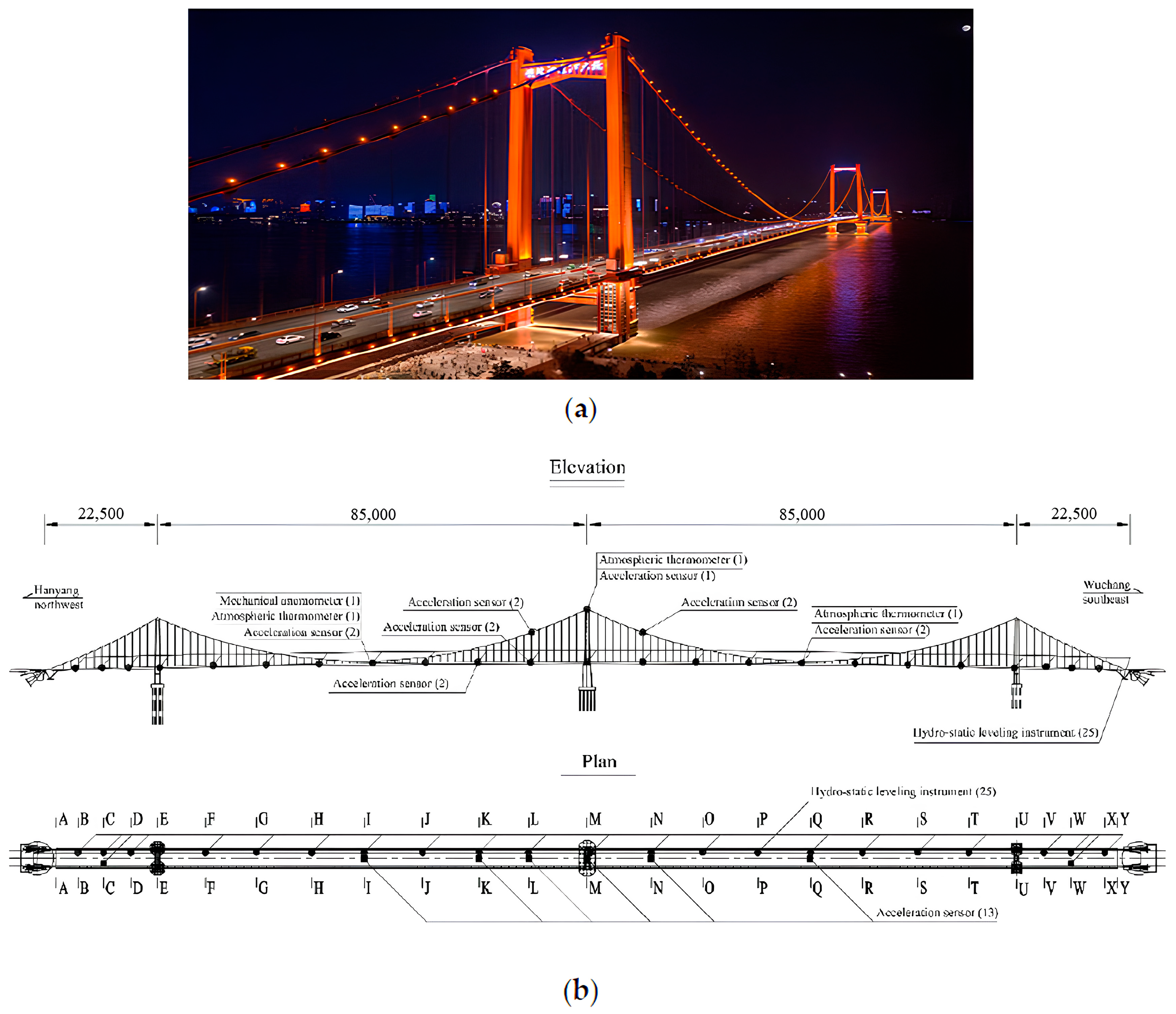
As previously mentioned, it is imperative to bridge the gap between theoretical concepts and practical applications in OSP. To accomplish this, it is crucial to showcase tangible instances where OSP techniques have proven effective in the context of engineering scenarios.

4.1. Bridges

Several studies have explored OSP for monitoring bridges in different locations. These studies utilize various techniques such as the effective independence approach, ant colony algorithm, MAC, and other optimization algorithms. Researchers have applied these methodologies to bridges in Poland, Spain, Dalian, Italy, Liaoning, Harbin, and Foshan, demonstrating the versatility and effectiveness of sensor placement for structural monitoring.

Figure 11 depicts the strategic arrangement of accelerometers on the Yingwuzhou Yangtze River Bridge, a three-tower, four-span suspension bridge, which extends 3.42 km in length, with its main span reaching 850 m, connecting Hanyang and Wuchang. It is equipped with an array of 58 sensors, including thermometers, anemometers, and accelerometers. These sensors facilitate real-time tracking of the bridge’s condition, ensuring its safety and operational integrity.

Moreover, Błachowski et al. [165] undertook OSP for load monitoring using the effective independence method, augmented by convex relaxation, on a tied-arch simply supported bridge situated in Poland. Pachón et al. [166] utilized the effective independence method to determine optimal sensor locations for the E. Torroja bridge, constructed in Spain in 1957. In a study by Feng et al. [167], an optimal arrangement method for triaxial sensors, complemented by the effective independence approach, was employed to assess the Dalian South Bay Cross-sea Bridge. Furthermore, Vincenzi et al. [168] introduced a novel methodology based on IE theory, integrating both distance and modal vectors, for OSP on a pedestrian bridge in Italy. These practical applications showcase the versatility and effectiveness of sensor placement methodologies across diverse structural scenarios.

Meanwhile, Feng et al. [169] introduced an arrangement method for triaxial acceleration sensors, leveraging the ant colony algorithm and MAC, and implemented this approach on the North Bridge in Dalian, Liaoning. Yang et al. [170] proposed a beetle-swarm evolution competitive algorithm with MAC as the objective function, effectively applied to a large-span bridge on the Haqi high-speed railroad in Harbin. Luo et al. [171] developed a novel harmony search cat swarm optimization algorithm, utilizing the MAC matrix’s non-diagonal element maxima as the evaluation criterion, which was successfully employed for the Beijiang Bridge in Foshan, Guangdong. Zhou et al. [88] innovatively merged the MAC evaluation criterion with considerations of wireless sensor connectivity and energy balance to formulate a hybrid discrete firefly algorithm, deployed on the Runyang Yangtze River Highway Bridge in Jiangsu Province.

Moreover, Xiao et al. [172] focuses on identifying damage in large-scale space truss structures using a stiffness separation method, particularly aimed at large-scale structures where traditional damage detection methods may be less effective due to the complexity and size of the structures. Later, by using numerical optimization, Xiao’s team determined the minimal number of sensors and their most effective layout for evaluating a bridge’s structural condition [173].

4.2. High-Rise Buildings

High-rise buildings, both current and future, have a significant need for SHM. In this part, studies have utilized different evaluation criteria such as MAC, MKE, and a combination of both. Researchers have conducted trials on diverse structures, including MIT campus buildings, the Canton Tower, Shanghai Center Tower, Shanghai Center Building, Jingji Financial Center, Dalian World Trade Center, and the Civil Engineering Research Building of National Taiwan University. The outcomes of these studies showcase the effectiveness and advantages of these innovative algorithms in achieving OSP for monitoring high-rise buildings and superstructures.

The Canton Tower in South China, standing at 610 m, is equipped with a long-term SHM system featuring over 700 sensors of 16 types. Ni et al. [174] developed a reduced-order FEM for benchmarking, comprising 37 beam elements and 185 DOFs, closely matching the full-scale FEM in modal frequencies and shapes. This benchmark study includes field data from 20 accelerometers, an anemometer, and a temperature sensor, along with details on sensor locations and specifications, as shown in Figure 12.

Additionally, Sun et al. [176] proposed a discrete optimization scheme based on an artificial bee colony algorithm, using MAC as the evaluation criterion, and conducted trials on various structures, including campus buildings at MIT and the iconic Canton Tower. Mahjoubi et al. [177] introduced a hypotrochoid spiral optimization algorithm to study optimal triaxial accelerometer placement for high-rise building monitoring. In an extensive evaluation using seven optimization algorithms, the efficiency of these approaches was assessed using the 632-m Shanghai Center Tower as a case study, with MAC as the key evaluation criterion. To realize the reconstruction of response to ground shaking, Hu et al. [178] applied a sequential sensor placement algorithm to achieve the OSP configuration with the minimum reconstruction error, and illustrated it with the example of Shanghai Center Building. By using the Jingji Financial Center as the engineering background, Fan et al. [179] studied the super high-rise construction monitoring system, applying the whole process of construction simulation technology to the OSP, according to the structural response changes in the process of construction simulation, to design a suitable temperature, vertical displacement, and stress measurement points placement scheme. Yi et al. [180] improved the monkey swarm algorithm and combined it with the MAC objective function to apply it in the Dalian World Trade Center, illustrating the advantages of the algorithm. Yang et al. [181] proposed an OSP method that can be used for structures that require repetitive monitoring to reduce the number of sensors required and to find the higher modal frequencies of the structure and illustrated the workability of the method by conducting a field test at the Civil Engineering Research Building of National Taiwan University. Mghazli et al. [163] combined the objective functions of MKE and MAC in a mixed meta-heuristic algorithm to design an OSP for the Willis Tower in Chicago and compared it with other algorithms to illustrate the effectiveness of the algorithm.

4.3. Others

Structures with complex designs, such as stadiums and museums, require SHM due to their architectural intricacies and high usage. SHM is essential for early detection of structural issues, ensuring safety, and preserving the integrity of these culturally significant buildings. This proactive approach is crucial for their long-term durability and safe operation.

The Shenzhen Sports Center spans 57,500 square meters and features a grandstand capable of seating approximately 45,000 spectators. The stadium is characterized by its elliptical grandstand, which measures 258 m along its major axis and 200 m along its minor axis, with the field’s main axis oriented north–south. The structure’s highest point reaches 32 m, featuring a grandstand that includes both upper and lower seating sections and a layer of private boxes sandwiched in between. The stadium is equipped with an SHM system that includes more than 100 sensors of four different types, strategically placed to monitor various critical points throughout the stadium, as shown in Figure 13.

Teng et al. [182] proposed a GA based on modal energy for optimal placement of multi-objective sensors and used the steel structure of the National Swimming Center as an engineering background to optimize the placement of acceleration sensors during its modal testing process. Xu et al. [183] used the particle swarm algorithm to optimize the arrangement of acceleration sensors and strain sensors in the monitoring system of Xining City Stadium, respectively. Jin et al. [184] used the effective independence method for OSP on the giant telescope cable network structure.

Wang et al. [185] proposed a new method named “Reduced Redundant Biaxial Modal Assurance Criteria” based on the three-dimensional modal assurance criterion for optimal placement of biaxial acceleration sensors and illustrated the advantages of the RRBMAC method with the example of a lattice transmission tower. Based on the ant colony optimization (ACO) algorithm, Feng et al. [186] proposed the “siege ant colony algorithm”, which aims to improve the efficiency and accuracy of the OSP problem in large-scale structure monitoring. The method is applied and compared with the standard method by using the Han River transmission tower as an example.

Schulze et al. [187] used a GA to minimize MAC non-diagonal elements to design an optimal solution for acceleration sensors for a 3-MWwind turbine. Cong et al. [188] developed a comprehensive strategy involving OSP, complex mode expansion, and cross-model cross-mode-based model updating technique. To demonstrate the effectiveness of the proposed method, computer simulations with the National Renewable Energy Laboratory 5-MW reference turbine are carried out.

Yan et al. [189] studied the method of OSP for offshore platforms using the example of an offshore platform in the South China Sea. Wang et al. [190] proposed an offshore platform sensor position fractional order optimization method and applied the effective independence method to experimentally study the fractional order placement of the sensors and validated the method with an offshore platform in Jinzhou as an example. A digital twin framework with OSP to accurately calculate the modal response and identify the damage rate of an offshore jacket platform was proposed by Wang et al. [191]. The OSP model was validated using a multi-objective Lichtenberg’s algorithm for sensor number/location optimization, and the proposed method was validated using an offshore jacket platform. These applications underscore the diverse range of innovative OSP for SHM.

4.4. Summary of the Section

This section has highlighted numerous successful applications of OSP techniques across a wide range of engineering scenarios. The research presented has optimized sensor configurations for bridge monitoring utilizing methods like the effective independence approach and MAC on structures in various locations worldwide. High-rise building monitoring studies have employed criteria such as MAC, modal kinetic energy, and their combination to determine OSP for tall buildings. Additionally, OSP has been featured for other structures including the swimming center, stadiums, telescope networks, transmission towers, wind turbines, and offshore platforms. Through diverse case studies evaluating different algorithms and metrics, this section underscores how OSP methods have been effectively deployed across this range of contexts to achieve practical, optimized solutions for SHM. These many examples showcase the versatility and demonstrate the value of employing theoretical frameworks for optimal sensor configuration in addressing real-world engineering challenges.

5. Challenges and Prospects

The previous sections provide an extensive review of OSP, covering its evolution, methodologies, primary research focus, and real-world applications in engineering. While the field has witnessed substantial growth, challenges still exist, which could guide future research directions.

5.1. Challenges

5.1.1. Interplay of Sensor Placement Sensing Techniques and Data Processing

The development of robust sensor networks for SHM must navigate the complex interplay between OSP, sensing techniques, and data processing. OSP plays a pivotal role in determining the physical locations of sensors, seeking to maximize spatial coverage and minimize resource expenditure. However, it must align with sensing techniques, which are critical when resources are scant, like in environmental monitoring, where visual sensing networks are advantageous for reducing sensor count without compromising data quality. Sensing techniques set the parameters for data collection, affecting both temporal and spatial data resolution, and consequently, the OSP strategy. Data processing techniques, such as compress sensing [192,193], offer a critical role in refining raw sensor data, enabling data quality enhancement and mitigation of suboptimal placement effects. Addressing this interplay calls for a comprehensive sensor network design strategy to achieve optimal performance and meet specific application needs.

5.1.2. The Bottleneck of Optimization Algorithms

The quest for a universally applicable algorithm is increasingly challenging due to the inherent diversity and complexity of real-world structural monitoring problems. The “no free lunch” theorem underscores that an algorithm’s efficacy depends on the specific problem it addresses, necessitating a strategic approach involving the development or selection of tailored evaluation criteria to align with distinct application needs. This customization of evaluation metrics enables optimization algorithms to be finely tuned, improving the computational efficiency of specific problem classes and ensuring a precise alignment of algorithmic solutions with unique application requirements.

5.1.3. Discrepancy between Research Advancements and Practical Applications

Many real-world applications still rely heavily on established guidelines and algorithms, highlighting an urgent need to more effectively integrate research findings into practical engineering applications. Future research in OSP should focus on closing this gap, adopting a pragmatic approach that emphasizes real-world applicability.

5.2. Prospects

5.2.1. Optimal Sensor Placement under Uncertainty

In practical engineering applications, it is imperative to consider factors such as structural modeling inaccuracies, device sampling precision, and measurement noise, all of which contribute to uncertainties in the identification of modal parameters. Therefore, when planning sensor placement, it becomes crucial to minimize these uncertainties, enhancing the overall stability and reliability of the sensor system. As an illustration, Lam et al. [14] addressed this challenge by modeling prediction errors as spatially correlated Gaussian processes, effectively resolving sensor redundancy and clustering issues. In a similar vein, Cantero-Chinchilla et al. [15] conducted research into optimal sensor configuration under conditions of parameter uncertainty. Their work encompassed aspects such as uncertainty in parameters, uncertainties in functions concerning parameters, and the spatial correlation of sensors.

5.2.2. Optimal Arrangement of Different Types of Sensors

In the field of SHM, according to the application of different purposes, the corresponding sensors are also different, such as acceleration sensors [122,167,169], which are commonly used in the vibration monitoring of the structure to obtain the dynamic information of the structure, such as frequency, damping ratio, etc.; fiber-optic strain sensors [194,195], which are commonly used in the strain monitoring of the structure to monitor fatigue rupture or corrosion, etc.; and temperature sensors [196,197,198], which are often used in cooperation with other sensors to monitor the effect of temperature changes on the structure. In addition to these popular sensors, there are also wind speed and direction sensors [199], inclination sensors [200], and so on. A single sensor type can only obtain part of the dynamic parameter information of the structure, and obtaining enough information about the structure requires the arrangement of multiple types of sensors; with sufficient information, a more comprehensive monitoring of the structure can be carried out.

A future development direction is how to use different types of sensors together to improve the monitoring effect. At present, scholars have carried out related research, such as the shifting of the OSP from a single type to a multi-type OSP and the performance of data acquisition and information fusion of multi-type sensors to improve the completeness of the sensor network. For example, Ručevskis et al. [86] investigated the problem of optimal arrangement of multiple types of sensors for damage and the identification of composite structures. Zhang et al. [33] proposed an algorithm for the optimal arrangement of multiple types of sensors.

5.2.3. Optimal Sensor Placement under Multiple Objectives

Current OSP methods primarily focus on the optimization of individual criteria such as modal independence, modal energy, system observability, and reliability. However, practical engineering applications often demand the satisfaction of multiple criteria simultaneously. In such scenarios, the optimization directions of each criterion may conflict with one another, and the magnitudes of evaluation criteria may not be consistent. Consequently, there is a growing need to explore multi-objective optimization methods that can strike a balance among different indicators. An example of such a method is NSGA-II [201], which is primarily designed for bi-objective optimization. For more complex multi-objective optimization scenarios, Deb et al. [202] introduced the NSGA-III algorithm in 2014, specifically tailored for handling problems with three to fifteen objectives. While research on OSP using the NSGA-II algorithm remains relatively limited, a few notable studies have emerged. For instance, Jiang et al. [203] defined a multi-objective optimization problem encompassing cost, reliability, and the implementation complexity of sensors, employing NSGA-II for OSP. Civera et al. [204] used the dual objective function of AutoMAC and CrossMAC with the NSGA-II algorithm to investigate Fossano’s church. Wang et al. [191] proposed a new digital twin (DT) framework based on optimal sensor placement for accurately calculating the modal response and identifying the damage rate of an offshore conduit rack platform. Its OSP model adopts the multi-objective Lichtenberg algorithm (MOLA) for optimizing the number and placement of sensors, which achieves a good balance between the cost of sensors and the accuracy of modal computation. Yang et al. [205] proposed an uncertainty-oriented multi-objective robust optimization method for optimal sensor placement by combining the traditional optimal sensor placement method with non-probability theory. The FIM and its uncertainty are taken as the first objective, and the minimum and mean values of the non-diagonal elements of the MAC matrix are taken as the second objective. An interval possibility is developed using the interval Pareto fronts to determine the optimal number of sensors.

Some researchers have also transformed it into a single-objective optimization problem by introducing weights for each indicator of the multi-objective function. Yang et al. [17] proposed an algorithm for structural health monitoring sensor placement based on an iterative updating process. The multi-objective function optimization is transformed into a single-objective optimization problem by considering the effects of different objective order differences. Zhang et al. [206] proposed a three-stage method for optimal sensor placement and developed a new logarithmic-type weighted fitting function for multi-type sensors and multi-objective monitoring, using a courtyard-style heritage built 133 years ago as an example.

It should be noted that how to strategically situate sensors to optimize multiple objectives is an important ongoing research direction. It is expected to propose new methods that can consider the influence of each parameter in the near future.

5.2.4. Optimal Sensor Placement with Emerging Technology

In the current landscape of sensor placement research, meta-heuristic algorithms are frequently employed to strike a balance between computational efficiency and accuracy. However, in situations where data is insufficient, these approaches can become inefficient and computationally expensive. To address these limitations, integrating AI techniques into the field of OSP presents a promising avenue. By harnessing extensive datasets to construct mapping networks, the potential exists to significantly enhance both computational efficiency and accuracy. A noteworthy illustration of this approach can be found in the work of Kaveh et al. [41], who incorporated reinforcement learning into OSP to optimize the computational efficiency of meta-heuristic algorithms.

6. Conclusions

In conclusion, OSP signifies an evolutionary stride in multidisciplinary integration, calling for a fluid incorporation into contemporary engineering methodologies and an embrace of insights from a plethora of technological fields. The pivotal steps in this intricate process are systematically outlined in Figure 14, which elucidates the dual objectives of this synthesis: to achieve cost-efficiency and to optimize performance in accordance with the demanding criteria of various engineering applications.

Our expansive review elucidates the pragmatic benefits of OSP within the realm of SHM, illustrated across diverse engineering scenarios. Case studies corroborate the effectiveness of selecting pertinent evaluation criteria that resonate with the specific goals of projects and the strategic employment of optimization algorithms. These approaches collectively yield advanced monitoring capabilities, manifesting in tangible advantages such as heightened accuracy in data reconstruction and the early detection of faults.

Extending beyond conventional civil structures, our investigation embraces a vast spectrum of applications, emphasizing the adaptability of optimization methodologies and the pivotal role of bespoke sensor planning. Looking ahead, we envision a future brightened by the advent of real-time sensor optimization through digital platforms, a development that hints at the transformative potential of collaborations between academic research and industry practices. Such synergies promise to substantially fortify the practices of structural monitoring. OSP techniques have evolved into a refined, data-centric tool poised to address the escalating demands of infrastructure and process monitoring.

Our research underlines the necessity of an all-encompassing approach that skillfully negotiates the interplay between coverage, precision, cost-effectiveness, and operational efficiency. OSP extends beyond the constraints of technical specifications, inviting a thoughtful contemplation of practicalities such as economic limitations, sensor availability, and environmental variables. The quest for optimal sensor locations unfolds as a multifarious challenge that demands the melding of disparate considerations to achieve specific monitoring objectives within the confines of logistical and fiscal realities. This paper shines a light on the nuanced equilibrium demanded by OSP, championing the development of bespoke, application-centric strategies within SHM. Our findings delineate OSP methodologies that stand out for their technical soundness and pragmatic viability, ensuring the deployment of sensor networks is as efficacious as it is attainable in tangible settings.

References

1. Omrany, H.; Ghaffarianhoseini, A.; Chang, R.D.; Ghaffarianhoseini, A.; Rahimian, F.P. Applications of Building information modelling in the early design stage of high-rise buildings. Autom. Constr. 2023, 152, 104934. [Google Scholar] [CrossRef]
2. Ni, F.T.; Zhang, J.; Noori, M.N. Deep learning for data anomaly detection and data compression of a long-span suspension bridge. Comput. Aided Civ. Infrastruct. Eng. 2020, 35, 685–700. [Google Scholar] [CrossRef]
3. Zhang, Y.M.; Wang, H.; Mao, J.X.; Xu, Z.D.; Zhang, Y.F. Probabilistic Framework with Bayesian Optimization Responses of a Long-Span Bridge. J. Struct. Eng. 2021, 147, 04020297. [Google Scholar] [CrossRef]
4. Xie, Z.H.; Xie, F.G.; Zhu, L.M.; Liu, X.J. Robotic mobile and mirror milling of large-scale complex structures. Natl. Sci. Rev. 2023, 10, nwac188. [Google Scholar] [CrossRef] [PubMed]
5. Yang, C. Advances and prospects for optimal sensor placement of structural health monitoring. J. Vib. Shock. 2020, 39, 82–93. [Google Scholar]
6. Tan, Y.; Zhang, L. Computational methodologies for optimal sensor placement in structural health monitoring: A review. Struct. Health Monit. 2019, 19, 1287–1308. [Google Scholar] [CrossRef]
7. Housner, G.W.; Bergman, L.A.; Caughey, T.K.; Chassiakos, A.G.; Claus, R.O.; Masri, S.F.; Skelton, R.E.; Soong, T.T.; Spencer, B.F.; Yao, J.T.P. Structural control: Past, present, and future. J. Eng. Mech. 1997, 123, 897–971. [Google Scholar] [CrossRef]
8. Yi, T.H.; Li, H.N. Methodology Developments in Sensor Placement for Health Monitoring of Civil Infrastructures. Int. J. Distrib. Sens. Netw. 2012, 11, 612726. [Google Scholar] [CrossRef]
9. Ostachowicz, W.; Soman, R.; Malinowski, P. Optimization of sensor placement for structural health monitoring: A review. Struct. Health Monit. 2019, 18, 963–988. [Google Scholar] [CrossRef]
10. Li, D.; Zhang, Y.; Ren, L.; Li, H. Sensor deployment for structural health monitoring and their evaluation. Adv. Mech. 2011, 41, 39–50. [Google Scholar]
11. Hernandez, E.M. Efficient sensor placement for state estimation in structural dynamics. Mech. Syst. Signal Proc. 2017, 85, 789–800. [Google Scholar] [CrossRef]
12. Leyder, C.; Dertimanis, V.; Frangi, A.; Chatzi, E.; Lombaert, G. Optimal sensor placement methods and metrics—Comparison and implementation on a timber frame structure. Struct. Infrastruct. Eng. 2018, 14, 997–1010. [Google Scholar] [CrossRef]
13. Lee, E.T.; Eun, H.C. An Optimal Sensor Layout Using the Frequency Response Function Data within a Wide Range of Frequencies. Sensors 2022, 22, 3778. [Google Scholar] [CrossRef] [PubMed]
14. Lam, H.-F.; Adeagbo, M.O. An enhanced sequential sensor optimization scheme and its application in the system identification of a rail-sleeper-ballast system. Mech. Syst. Signal Proc. 2022, 163, 108188. [Google Scholar] [CrossRef]
15. Cantero-Chinchilla, S.; Papadimitriou, C.; Chiachío, J.; Chiachío, M.; Koumoutsakos, P.; Fabro, A.T.; Chronopoulos, D. Robust optimal sensor configuration using the value of information. Struct. Control Health Monit. 2022, 29, e3143. [Google Scholar] [CrossRef]
16. Loutas, T.H.; Bourikas, A. Strain sensors optimal placement for vibration-based structural health monitoring. The effect of damage on the initially optimal configuration. J. Sound. Vib. 2017, 410, 217–230. [Google Scholar] [CrossRef]
17. Yang, C. An adaptive sensor placement algorithm for structural health monitoring based on multi-objective iterative optimization using weight factor updating. Mech. Syst. Signal Proc. 2021, 151, 107363. [Google Scholar] [CrossRef]
18. Lin, J.-F.; Xu, Y.-L. Response covariance-based sensor placement for structural damage detection. Struct. Infrastruct. Eng. 2017, 14, 1207–1220. [Google Scholar] [CrossRef]
19. Yang, C.; Lu, Z. An interval effective independence method for optimal sensor placement based on non-probabilistic approach. Sci. China Technol. Sci. 2016, 60, 186–198. [Google Scholar] [CrossRef]
20. Bertola, N.J.; Smith, I.F.C. A methodology for measurement-system design combining information from static and dynamic excitations for bridge load testing. J. Sound. Vib. 2019, 463, 114953. [Google Scholar] [CrossRef]
21. Kim, T.; Youn, B.D.; Oh, H. Development of a stochastic effective independence (SEFI) method for optimal sensor placement under uncertainty. Mech. Syst. Signal Proc. 2018, 111, 615–627. [Google Scholar] [CrossRef]
22. Zhang, Y.; Chai, S.; An, C.; Lim, F.; Duan, M. A new method for optimal sensor placement considering multiple factors and its application to deepwater riser monitoring systems. Ocean. Eng. 2022, 244, 110403. [Google Scholar] [CrossRef]
23. Downey, A.; Hu, C.; Laflamme, S. Optimal sensor placement within a hybrid dense sensor network using an adaptive genetic algorithm with learning gene pool. Struct. Health Monit. 2017, 17, 450–460. [Google Scholar] [CrossRef]
24. Yang, C.; Lu, Z.; Yang, Z. Robust Optimal Sensor Placement for Uncertain Structures with Interval Parameters. IEEE Sens. J. 2018, 18, 2031–2041. [Google Scholar] [CrossRef]
25. Yi, T.H.; Zhou, G.D.; Li, H.N.; Wang, C.W. Optimal placement of triaxial sensors for modal identification using hierarchic wolf algorithm. Struct. Control. Health Monit. 2017, 24, e1958. [Google Scholar] [CrossRef]
26. Yang, C.; Zheng, W.; Zhang, X. Optimal sensor placement for spatial lattice structure based on three-dimensional redundancy elimination model. Appl. Math. Model. 2019, 66, 576–591. [Google Scholar] [CrossRef]
27. Su, J.-B.; Luan, S.-L.; Zhang, L.-M.; Zhu, R.-H.; Qin, W.-G. Partitioned genetic algorithm strategy for optimal sensor placement based on structure features of a high-piled wharf. Struct. Control Health Monit. 2019, 26, e2289. [Google Scholar] [CrossRef]
28. Yang, C.; Xia, Y. A novel two-step strategy of non-probabilistic multi-objective optimization for load-dependent sensor placement with interval uncertainties. Mech. Syst. Signal Proc. 2022, 176, 109173. [Google Scholar] [CrossRef]
29. Colombo, L.; Todd, M.D.; Sbarufatti, C.; Giglio, M. On statistical Multi-Objective optimization of sensor networks and optimal detector derivation for structural health monitoring. Mech. Syst. Signal Proc. 2022, 167, 108528. [Google Scholar] [CrossRef]
30. Yuen, K.V.; Hao, X.H.; Kuok, S.C. Robust sensor placement for structural identification. Struct. Control. Health Monit. 2022, 29, e2861. [Google Scholar] [CrossRef]
31. Shi, Q.; Wang, H.; Wang, L.; Luo, Z.; Wang, X.; Han, W. A bilayer optimization strategy of optimal sensor placement for parameter identification under uncertainty. Struct. Multidiscip. Optim. 2022, 65, 264. [Google Scholar] [CrossRef]
32. Nieminen, V.; Sopanen, J. Optimal sensor placement of triaxial accelerometers for modal expansion. Mech. Syst. Signal Proc. 2023, 184, 109581. [Google Scholar] [CrossRef]
33. Zhang, C.D.; Xu, Y.L. Optimal multi-type sensor placement for response and excitation reconstruction. J. Sound. Vib. 2016, 360, 112–128. [Google Scholar] [CrossRef]
34. Mendler, A.; Döhler, M.; Ventura, C.E. Sensor placement with optimal damage detectability for statistical damage detection. Mech. Syst. Signal Proc. 2022, 170, 108767. [Google Scholar] [CrossRef]
35. Zhang, C.; Zhou, Z.; Hu, G.; Yang, L.; Tang, S. Health assessment of the wharf based on evidential reasoning rule considering optimal sensor placement. Measurement 2021, 186, 110184. [Google Scholar] [CrossRef]
36. Dinh-Cong, D.; Dang-Trung, H.; Nguyen-Thoi, T. An efficient approach for optimal sensor placement and damage identification in laminated composite structures. Adv. Eng. Softw. 2018, 119, 48–59. [Google Scholar] [CrossRef]
37. Chisari, C.; Macorini, L.; Amadio, C.; Izzuddin, B.A. Optimal sensor placement for structural parameter identification. Struct. Multidiscip. Optim. 2016, 55, 647–662. [Google Scholar] [CrossRef]
38. Huang, Y.; Ludwig, S.A.; Deng, F. Sensor optimization using a genetic algorithm for structural health monitoring in harsh environments. J. Civ. Struct. Health Monit. 2016, 6, 509–519. [Google Scholar] [CrossRef]
39. Lin, C.; Zhang, C.-l.; Chen, J.-h. Optimal arrangement of structural sensors in soft rock tunnels based industrial IoT applications. Comput. Commun. 2020, 156, 159–167. [Google Scholar] [CrossRef]
40. Keskin, M.E. A column generation heuristic for optimal wireless sensor network design with mobile sinks. Eur. J. Oper. Res. 2017, 260, 291–304. [Google Scholar] [CrossRef]
41. Kaveh, A.; Dadras Eslamlou, A.; Rahmani, P.; Amirsoleimani, P. Optimal sensor placement in large-scale dome trusses via Q-learning-based water strider algorithm. Struct. Control Health Monit. 2022, 29, e2949. [Google Scholar] [CrossRef]
42. Zhou, S.; Yu, L.; Wu, Z.; Yang, H. Optimal Sensor Placement Based on Deep Learning Method. J. Vib. Meas. Diagn. 2020, 40, 719–724. [Google Scholar]
43. Salama, M.; Rose, T.; Garba, J. Optimal placement of excitations and sensors for verification of large dynamical systems. In Proceedings of the 28th Structures, Structural Dynamics and Materials Conference, Monterey, CA, USA, 6–8 April 1987. [Google Scholar]
44. Stubbs, N.; Kim, J.T. Damage localization in structures without baseline modal parameters. Aiaa J. 1996, 34, 1644–1649. [Google Scholar] [CrossRef]
45. Kim, J.T.; Ryu, Y.S.; Cho, H.M.; Stubbs, N. Damage identification in beam-type structures: Frequency-based method vs mode-shape-based method. Eng. Struct. 2003, 25, 57–67. [Google Scholar] [CrossRef]
46. He, C.; Xing, J.; Li, J.; Yang, Q.; Wang, R.; Zhang, X. A Combined Optimal Sensor Placement Strategy for the Structural Health Monitoring of Bridge Structures. Int. J. Distrib. Sens. Netw. 2013, 9, 820694. [Google Scholar] [CrossRef]
47. Declerck, J.P.; Avitabile, P. Development of Several New Tools for Modal Pre-test Evaluation. In Proceedings of the 14th International Modal Analysis Conference, Dearborn, MI, USA, 12–15 February 1996; p. 1272. [Google Scholar]
48. Horn, R.A.; Johnson, C.R. Matrix Analysis; Cambridge University Press: Cambridge, UK, 2012. [Google Scholar]
49. Gui, C.; Lei, J.; Duan, Z.; Zhang, X. Optimal sensor placement by using MSSP/DM-MAC method. Chin. J. Appl. Mech. 2019, 36, 1499–1503. [Google Scholar]
50. Heylen, W.; Lammens, S.; Sas, P. Modal Analysis Theory and Testing; Katholieke Universiteit Leuven: Leuven, Belgium, 1997; Volume 200. [Google Scholar]
51. Larson, C.B.; Zimmerman, D.C.; Marek, E.L. A comparison of modal test planning techniques: Excitation and sensor placement using the NASA 8-bay truss. In Proceedings of the 12th International Modal Analysis Conference, Ilikai Hotel, Honolulu, HI, USA, 31 January–3 February 1994; Volume 2251, p. 205. [Google Scholar]
52. Imamovic, N.; Ewins, D. Optimization of excitation DOF selection for modal tests. In Proceedings of the 15th International Modal Analysis Conference, Orlando, FL, USA, 3–6 February 1997; p. 1945. [Google Scholar]
53. Imamovic, N. Validation of Large Structural dynamics MODELS Using Modal Test Data. Doctoral Dissertation, Department of Mechanical Engineering, Imperial College, London, UK, 1998. [Google Scholar]
54. Meo, M.; Zumpano, G. On the optimal sensor placement techniques for a bridge structure. Eng. Struct. 2005, 27, 1488–1497. [Google Scholar] [CrossRef]
55. Carne, T.G.; Dohrmann, C.R. A modal test design strategy for model correlation. In Proceedings of the Conference: International Modal Analysis Conference, Nashville, TN, USA, 13–16 February 1995. [Google Scholar]
56. An, H.; Youn, B.D.; Kim, H.S. A methodology for sensor number and placement optimization for vibration-based damage detection of composite structures under model uncertainty. Compos. Struct. 2022, 279, 114863. [Google Scholar] [CrossRef]
57. Stephan, C. Sensor placement for modal identification. Mech. Syst. Signal Proc. 2012, 27, 461–470. [Google Scholar] [CrossRef]
58. Lin, T.Y.; Tao, J.; Huang, H.H. A Multiobjective Perspective to Optimal Sensor Placement by Using a Decomposition-Based Evolutionary Algorithm in Structural Health Monitoring. Appl. Sci. 2020, 10, 7710. [Google Scholar] [CrossRef]
59. Golub, G.H.; Van Loan, C.F. Matrix Computations; JHU Press: Baltimore, MD, USA, 2013. [Google Scholar]
60. Cherng, A.P. Optimal sensor placement for modal parameter identification using signal subspace correlation techniques. Mech. Syst. Signal Proc. 2003, 17, 361–378. [Google Scholar] [CrossRef]
61. Chhabra, D.; Bhushan, G.; Chandna, P. Optimal placement of piezoelectric actuators on plate structures for active vibration control via modified controlmatrix and singular value decomposition approach using modified heuristic genetic algorithm. Mech. Adv. Mater. Struct. 2016, 23, 272–280. [Google Scholar] [CrossRef]
62. Kammer, D.C. Sensor placement for on-orbit modal identification and correlation of large space structures. J. Guid. Control Dyn. 1991, 14, 251–259. [Google Scholar] [CrossRef]
63. Bayard, D.S.; Hadaegh, F.Y.; Meldrum, D.R. Optimal experiment design for identification of large space structures. Automatica 1988, 24, 357–364. [Google Scholar] [CrossRef]
64. Borguet, S.; Leonard, O. The Fisher Information Matrix as a Relevant Tool for Sensor Selection in Engine Health Monitoring. Int. J. Rotating Mach. 2008, 2008, 784749. [Google Scholar] [CrossRef]
65. An, H.; Youn, B.D.; Kim, H.S. Optimal Sensor Placement Considering Both Sensor Faults under Uncertainty and Sensor Clustering for Vibration-Based Damage Detection. Struct. Multidiscip. Optim. 2022, 65, 102. [Google Scholar] [CrossRef]
66. Papadimitriou, C.; Beck, J.L.; Au, S.K. Entropy-based optimal sensor location for structural model updating. J. Vib. Control 2000, 6, 781–800. [Google Scholar] [CrossRef]
67. Papadimitriou, C. Pareto optimal sensor locations for structural identification. Comput. Meth. Appl. Mech. Eng. 2005, 194, 1655–1673. [Google Scholar] [CrossRef]
68. Papadimitriou, C. Optimal sensor placement methodology for parametric identification of structural systems. J. Sound. Vib. 2004, 278, 923–947. [Google Scholar] [CrossRef]
69. Yang, Y.; Chadha, M.; Hu, Z.; Todd, M.D. An optimal sensor placement design framework for structural health monitoring using Bayes risk. Mech. Syst. Signal Proc. 2022, 168, 108618. [Google Scholar] [CrossRef]
70. Bansal, S.; Cheung, S.H. On the Bayesian sensor placement for two-stage structural model updating and its validation. Mech. Syst. Signal Proc. 2022, 169, 108578. [Google Scholar] [CrossRef]
71. Pei, X.-Y.; Yi, T.-H.; Qu, C.-X.; Li, H.-N. Conditional information entropy based sensor placement method considering separated model error and measurement noise. J. Sound. Vib. 2019, 449, 389–404. [Google Scholar] [CrossRef]
72. Mehrjoo, A.; Song, M.; Moaveni, B.; Papadimitriou, C.; Hines, E. Optimal sensor placement for parameter estimation and virtual sensing of strains on an offshore wind turbine considering sensor installation cost. Mech. Syst. Signal Proc. 2022, 169, 108787. [Google Scholar] [CrossRef]
73. Said, W.M.; Staszewski, W.J. Optimal sensor location for damage detection using mutual information. In Proceedings of the 11th International Conference on Adaptive Structures and Technologies (ICAST), Nagoya, Japan, 23–26 October 2000; pp. 428–435. [Google Scholar]
74. Chen, M.J.; Sivakumar, K.; Banyay, G.A.; Golchert, B.M.; Walsh, T.F.; Zavlanos, M.M.; Aquino, W. Bayesian Optimal Sensor Placement for Damage Detection in Frequency-Domain Dynamics. J. Eng. Mech. 2022, 148, 04022078. [Google Scholar] [CrossRef]
75. Bhattacharyya, P.; Beck, J. Exploiting convexification for Bayesian optimal sensor placement by maximization of mutual information. Struct. Control. Health Monit. 2020, 27, e2605. [Google Scholar] [CrossRef]
76. Azam, S.E.; Chatzi, E.; Papadimitriou, C. A dual Kalman filter approach for state estimation via output-only acceleration measurements. Mech. Syst. Signal Proc. 2015, 60–61, 866–886. [Google Scholar] [CrossRef]
77. O’Callahan, J.C. System equivalent reduction expansion process. In Proceedings of the 7th International Modal Analysis Conference, Las Vegas, NV, USA, 30 January–2 February 1989. [Google Scholar]
78. O’Callahan, J.; Li, P. A non smoothing SEREP process for modal expansion. In Proceedings of the 12th International Modal Analysis Conference, Ilikai Hotel, Honolulu, HI, USA, 31 January–3 February 1994; Volume 2251, p. 232. [Google Scholar]
79. Guyan, R.J. Reduction of stiffness and mass matrices. Aiaa J. 1965, 3, 380. [Google Scholar] [CrossRef]
80. Lin, J.F.; Xu, Y.L.; Law, S.S. Structural damage detection-oriented multi-type sensor placement with multi-objective optimization. J. Sound. Vib. 2018, 422, 568–589. [Google Scholar] [CrossRef]
81. Nasr, D.; Dahr, R.E.; Assaad, J.; Khatib, J. Comparative Analysis between Genetic Algorithm and Simulated Annealing-Based Frameworks for Optimal Sensor Placement and Structural Health Monitoring Purposes. Buildings 2022, 12, 1383. [Google Scholar] [CrossRef]
82. Jaya, M.M.; Ceravolo, R.; Fragonara, L.Z.; Matta, E. An optimal sensor placement strategy for reliable expansion of mode shapes under measurement noise and modelling error. J. Sound. Vib. 2020, 487, 115511. [Google Scholar] [CrossRef]
83. Cumbo, R.; Tamarozzi, T.; Janssens, K.; Desmet, W. Kalman-based load identification and full-field estimation analysis on industrial test case. Mech. Syst. Signal Proc. 2019, 117, 771–785. [Google Scholar] [CrossRef]
84. Warsewa, A.; Bohm, M.; Guerra, F.; Wagner, J.L.; Haist, T.; Tarin, C.; Sawodny, O. Self-tuning state estimation for adaptive truss structures using strain gauges and camera-based position measurements. Mech. Syst. Signal Proc. 2020, 143, 106822. [Google Scholar] [CrossRef]
85. Flynn, E.B.; Todd, M.D. A Bayesian approach to optimal sensor placement for structural health monitoring with application to active sensing. Mech. Syst. Signal Proc. 2010, 24, 891–903. [Google Scholar] [CrossRef]
86. Rucevskis, S.; Rogala, T.; Katunin, A. Optimal Sensor Placement for Modal-Based Health Monitoring of a Composite Structure. Sensors 2022, 22, 3867. [Google Scholar] [CrossRef] [PubMed]
87. Hou, R.R.; Xia, Y.; Xia, Q.; Zhou, X.Q. Genetic algorithm based optimal sensor placement for L-1-regularized damage detection. Struct. Control. Health Monit. 2019, 26, e2274. [Google Scholar] [CrossRef]
88. Zhou, G.D.; Yi, T.H.; Zhang, H.; Li, H.N. Energy-aware wireless sensor placement in structural health monitoring using hybrid discrete firefly algorithm. Struct. Control. Health Monit. 2015, 22, 648–666. [Google Scholar] [CrossRef]
89. Elsersy, M.; Elfouly, T.M.; Ahmed, M.H. Joint Optimal Placement, Routing, and Flow Assignment in Wireless Sensor Networks for Structural Health Monitoring. IEEE Sens. J. 2016, 16, 5095–5106. [Google Scholar] [CrossRef]
90. Liu, Y.; Chin, K.W.; Yang, C.L.; He, T.J. Nodes Deployment for Coverage in Rechargeable Wireless Sensor Networks. IEEE Trans. Veh. Technol. 2019, 68, 6064–6073. [Google Scholar] [CrossRef]
91. Tam, N.T.; Binh, H.T.T.; Dat, V.T.; Lan, P.N.; Vinh, L.T. Towards optimal wireless sensor network lifetime in three dimensional terrains using relay placement metaheuristics. Knowl.-Based Syst. 2020, 206, 106407. [Google Scholar] [CrossRef]
92. Yuan, B.; Chen, H.H.; Yao, X. Optimal relay placement for lifetime maximization in wireless underground sensor networks. Inf. Sci. 2017, 418, 463–479. [Google Scholar] [CrossRef]
93. Hao, X.H.; Yuen, K.V.; Kuok, S.C. Energy-aware versatile wireless sensor network configuration for structural health monitoring. Struct. Control. Health Monit. 2022, 29, e3083. [Google Scholar] [CrossRef]
94. Xenakis, A.; Foukalas, F.; Stamoulis, G. Cross-layer energy-aware topology control through Simulated Annealing for WSNs. Comput. Electr. Eng. 2016, 56, 576–590. [Google Scholar] [CrossRef]
95. Fang, K.; Liu, C.Y.; Teng, J. Cluster-based optimal wireless sensor deployment for structural health monitoring. Struct. Health Monit. 2018, 17, 266–278. [Google Scholar] [CrossRef]
96. Juhlin, M.; Jakobsson, A. Optimal sensor placement for localizing structured signal sources. Signal Process. 2023, 202, 108679. [Google Scholar] [CrossRef]
97. Dhillon, S.S.; Chakrabarty, K. Sensor placement for effective coverage and surveillance in distributed sensor networks. In Proceedings of the 2003 IEEE Wireless Communications and Networking, WCNC 2003, New Orleans, LA, USA, 16–20 March 2003; Volume 1603, pp. 1609–1614. [Google Scholar]
98. Maulin, P.; Chandrasekaran, R.; Venkatesan, S. Energy efficient sensor, relay and base station placements for coverage, connectivity and routing. In Proceedings of the PCCC 2005, 24th IEEE International Performance, Computing, and Communications Conference, Phoenix, AZ, USA, 7–9 April 2005; pp. 581–586. [Google Scholar]
99. Wang, B. Coverage problems in sensor networks: A survey. ACM Comput. Surv. 2011, 43, 32. [Google Scholar] [CrossRef]
100. Wu, H.; Liu, Z.; Hu, J.; Yin, W. Sensor placement optimization for critical-grid coverage problem of indoor positioning. Int. J. Distrib. Sens. Netw. 2020, 16. [Google Scholar] [CrossRef]
101. Akbarzadeh, V.; Lévesque, J.C.; Gagné, C.; Parizeau, M. Efficient sensor placement optimization using gradient descent and probabilistic coverage. Sensors 2014, 14, 15525–15552. [Google Scholar] [CrossRef]
102. Thiene, M.; Khodaei, Z.S.; Aliabadi, M.H. Optimal sensor placement for maximum area coverage (MAC) for damage localization in composite structures. Smart Mater. Struct. 2016, 25, 095037. [Google Scholar] [CrossRef]
103. Liu, J.; Ouyang, H.; Han, X.; Liu, G.R. Optimal sensor placement for uncertain inverse problem of structural parameter estimation. Mech. Syst. Signal Proc. 2021, 160, 107914. [Google Scholar] [CrossRef]
104. Sadhu, A.; Goli, G. Blind source separation-based optimum sensor placement strategy for structures. J. Civ. Struct. Health Monit. 2017, 7, 445–458. [Google Scholar] [CrossRef]
105. Biswal, S.; Wang, Y. Optimal sensor placement strategy for the identification of local bolted connection failures in steel structures. In Proceedings of the International Conference on Smart Infrastructure and Construction 2019 (ICSIC), 2019 Churchill College, Cambridge, UK, 8–10 July 2019. [Google Scholar]
106. Shi, Q.H.; Wang, X.J.; Chen, W.P.; Hu, K.J. Optimal Sensor Placement Method Considering the Importance of Structural Performance Degradation for the Allowable Loadings for Damage Identification. Appl. Math. Model. 2020, 86, 384–403. [Google Scholar] [CrossRef]
107. Ghosh, D.; Mukhopadhyay, S. Fisher information-based optimal sensor locations for output-only structural identification under base excitation. Struct. Control. Health Monit. 2022, 29, e3021. [Google Scholar] [CrossRef]
108. Luenberger, D.G.; Ye, Y. Linear and Nonlinear Programming; Springer: Reading, MA, USA, 1984; Volume 2. [Google Scholar]
109. Deuflhard, P. Newton Methods for Nonlinear Problems: Affine Invariance and Adaptive Algorithms; Springer Science & Business Media: New York, NY, USA, 2005; Volume 35. [Google Scholar]
110. Sepulveda, A.E.; Jin, I.M.; Schmit, L.A. Optimal placement of active elements in control augmented structural synthesis. Aiaa J. 1993, 31, 1906–1915. [Google Scholar] [CrossRef]
111. Cruz, A.; Velez, W.; Thomson, P. Optimal sensor placement for modal identification of structures using genetic algorithms-a case study: The olympic stadium in Cali, Colombia. Ann. Oper. Res. 2010, 181, 769–781. [Google Scholar] [CrossRef]
112. Li, D.-S.; Fritzen, C.-P.; Li, H.-N. Extended MinMAC algorithm and comparison of sensor placement methods. In Proceedings of the IMAC-XXVI, Orlando, FL, USA, 4–7 February 2008. [Google Scholar]
113. Holland, J.H. Adaptation in Natural and Artificial Systems: An Introductory Analysis with Applications to Biology, Control, and Artificial Intelligence; MIT Press: Cambridge, MA, USA, 1992. [Google Scholar]
114. Zhou, K.; Wu, Z.Y. Strain gauge placement optimization for structural performance assessment. Eng. Struct. 2017, 141, 184–197. [Google Scholar] [CrossRef]
115. Cazzulani, G.; Chieppi, M.; Colombo, A.; Pennacchi, P. Optimal sensor placement for continuous optical fiber sensors. In Proceedings of the Conference on Sensors and Smart Structures Technologies for Civil, Mechanical, and Aerospace Systems, Denver, CA, USA, 5–8 March 2018. [Google Scholar]
116. Rao, A.R.M.; Anandakumar, G. Optimal placement of sensors for structural system identification and health monitoring using a hybrid swarm intelligence technique. Smart Mater. Struct. 2007, 16, 2658–2672. [Google Scholar] [CrossRef]
117. Overton, G.; Worden, K. Sensor optimisation using an ant colony metaphor. Strain 2004, 40, 59–65. [Google Scholar] [CrossRef]
118. Scott, M.; Worden, K. A Bee Swarm Algorithm for Optimising Sensor Distributions for Impact Detection on a Composite Panel. Strain 2015, 51, 147–155. [Google Scholar] [CrossRef]
119. Yi, T.H.; Li, H.N.; Zhang, X.D. Health monitoring sensor placement optimization for Canton Tower using immune monkey algorithm. Struct. Control. Health Monit. 2015, 22, 123–138. [Google Scholar] [CrossRef]
120. Zhou, G.-D.; Yi, T.-H.; Li, H.-N. Sensor placement optimization in structural health monitoring using cluster-in-cluster firefly algorithm. Adv. Struct. Eng. 2014, 17, 1103–1115. [Google Scholar] [CrossRef]
121. Gao, H.D.; Rose, J.L. Sensor placement optimization in structural health monitoring using genetic and evolutionary algorithms. In Proceedings of the Smart Structures and Materials 2006 Conference, San Diego, CA, USA, 27 February–2 March 2006. [Google Scholar]
122. Yi, T.H.; Li, H.N.; Gu, M. Optimal Sensor Placement for Health Monitoring of High-Rise Structure Based on Genetic Algorithm. Math. Probl. Eng. 2011, 2011, 395101. [Google Scholar] [CrossRef]
123. Roy, T.; Chakraborty, D. Optimal vibration control of smart fiber reinforced composite shell structures using improved genetic algorithm. J. Sound. Vib. 2009, 319, 15–40. [Google Scholar] [CrossRef]
124. Zhang, H.W.; Lennox, B.; Goulding, P.R.; Leung, A.Y.T. A float-encoded genetic algorithm technique for integrated optimization of piezoelectric actuator and sensor placement and feedback gains. Smart Mater. Struct. 2000, 9, 552–557. [Google Scholar] [CrossRef]
125. Liu, W.; Gao, W.C.; Sun, Y.; Xu, M.J. Optimal sensor placement for spatial lattice structure based on genetic algorithms. J. Sound. Vib. 2008, 317, 175–189. [Google Scholar] [CrossRef]
126. Zhu, K.; Gu, C.S.; Qiu, J.C.; Liu, W.X.; Fang, C.H.; Li, B. Determining the Optimal Placement of Sensors on a Concrete Arch Dam Using a Quantum Genetic Algorithm. J. Sens. 2016, 2016, 2567305. [Google Scholar] [CrossRef]
127. Minshui, H.; Jie, L.; Hongping, Z. Optimal sensor layout for bridge health monitoring based on dual-structure coding genetic algorithm. In Proceedings of the 2009 International Conference on Computational Intelligence and Software Engineering, Wuhan, China, 1–13 December 2009; p. 4. [Google Scholar] [CrossRef]
128. Katoch, S.; Chauhan, S.S.; Kumar, V. A review on genetic algorithm: Past, present, and future. Multimed. Tools Appl. 2021, 80, 8091–8126. [Google Scholar] [CrossRef]
129. Fox, B.; McMahon, M. Genetic operators for sequencing problems. In Foundations of Genetic Algorithms; Elsevier: Amsterdam, The Netherlands, 1991; Volume 1, pp. 284–300. [Google Scholar]
130. Jebari, K.; Madiafi, M. Selection methods for genetic algorithms. Int. J. Emerg. Sci. 2013, 3, 333–344. [Google Scholar]
131. Soon, G.K.; Guan, T.T.; On, C.K.; Alfred, R.; Anthony, P. A Comparison on the Performance of Crossover Techniques in Video Game. In Proceedings of the IEEE International Conference on Control System, Computing and Engineering (ICCSCE), Penang, Malaysia, 29 November–1 December 2013; pp. 493–498. [Google Scholar]
132. Goldberg, D.E.; Lingle, R. Alleles, loci, and the traveling salesman problem. In Proceedings of the First International Conference on Genetic Algorithms and Their Applications; L. Erlbaum Associates Inc.: Hillsdale, NJ, USA, 1985; pp. 154–159. [Google Scholar]
133. Buczak, A.L.; Wang, H.; Darabi, H.; Jafari, M.A.; Jafari, B. Genetic algorithm convergence study for sensor network optimization. Inf. Sci. 2001, 133, 267–282. [Google Scholar] [CrossRef]
134. Maul, W.A.; Kopasakis, G.; Santi, L.M.; Sowers, T.S.; Chicatelli, A. Sensor Selection and Optimization for Health Assessment of Aerospace Systems. J. Aerosp. Comput. Inf. Commun. 2008, 5, 16–34. [Google Scholar] [CrossRef]
135. Wolpert, D.H.; Macready, W.G. No free lunch theorems for optimization. IEEE Trans. Evol. Comput. 1997, 1, 67–82. [Google Scholar] [CrossRef]
136. Liu, H.B.; Wu, C.L.; Wang, J. Sensor Optimal Placement for Bridge Structure based on Single Parents Genetic Algorithm with Different Fitness Functions. In Bridge Health Monitoring, Maintenance and Safety; Liu, Y., Ed.; Key Engineering Materials; Trans Tech Publications Ltd.: Durnten, Switzerland; Zurich, Switzerland, 2011; Volume 456, pp. 115–124. [Google Scholar]
137. Kang, F.; Li, J.J.; Xu, Q. Virus coevolution partheno-genetic algorithms for optimal sensor placement. Adv. Eng. Inform. 2008, 22, 362–370. [Google Scholar] [CrossRef]
138. Nandy, A.; Chakraborty, D.; Shah, M.S. Optimal Sensors/Actuators Placement in Smart Structure Using Island Model Parallel Genetic Algorithm. Int. J. Comput. Methods 2019, 16, 1840018. [Google Scholar] [CrossRef]
139. Ganesan, T.; Rajarajeswari, P. Efficient sensor node connectivity and target coverage using genetic algorithm with Daubechies 4 lifting wavelet transform. Int. J. Commun. Netw. Distrib. Syst. 2022, 28, 337–364. [Google Scholar] [CrossRef]
140. Kim, C.; Oh, H.; Jung, B.C.; Moon, S.J. Optimal sensor placement to detect ruptures in pipeline systems subject to uncertainty using an Adam-mutated genetic algorithm. Struct. Health Monit. 2022, 21, 2354–2369. [Google Scholar] [CrossRef]
141. Qin, X.R.; Zhan, P.M.; Yu, C.Q.; Zhang, Q.; Sun, Y.T. Health monitoring sensor placement optimization based on initial sensor layout using improved partheno-genetic algorithm. Adv. Struct. Eng. 2021, 24, 252–265. [Google Scholar] [CrossRef]
142. Kennedy, J.; Eberhart, R. Particle swarm optimization. In Proceedings of the 1995 IEEE International Conference on Neural Networks Proceedings (Cat. No.95CH35828), Perth, WA, Australia, 27 November–1 December 1995; Volume 1944, pp. 1942–1948. [Google Scholar] [CrossRef]
143. Hassani, S.; Dackermann, U. A Systematic Review of Optimization Algorithms for Structural Health Monitoring and Optimal Sensor Placement. Sensors 2023, 23, 3293. [Google Scholar] [CrossRef] [PubMed]
144. Deng, Z.H.; Huang, M.S.; Wan, N.; Zhang, J.W. The Current Development of Structural Health Monitoring for Bridges: A Review. Buildings 2023, 13, 1360. [Google Scholar] [CrossRef]
145. Jain, M.; Saihjpal, V.; Singh, N.; Singh, S.B. An Overview of Variants and Advancements of PSO Algorithm. Appl. Sci. 2022, 12, 8392. [Google Scholar] [CrossRef]
146. Shi, Y.; Eberhart, R. A modified particle swarm optimizer. In Proceedings of the 1998 IEEE International Conference on Evolutionary Computation Proceedings, IEEE World Congress on Computational Intelligence (Cat. No.98TH8360), Anchorage, AK, USA, 4–9 May 1998; pp. 69–73. [Google Scholar] [CrossRef]
147. Wang, L.; Ye, W.; Wang, H.K.; Fu, X.P.; Fei, M.R.; Menhas, M.I. Optimal Node Placement of Industrial Wireless Sensor Networks Based on Adaptive Mutation Probability Binary Particle Swarm Optimization Algorithm. Comput. Sci. Inf. Syst. 2012, 9, 1553–1576. [Google Scholar] [CrossRef]
148. He, L.J.; Lian, J.J.; Ma, B.; Wang, H.J. Optimal multiaxial sensor placement for modal identification of large structures. Struct. Control. Health Monit. 2014, 21, 61–79. [Google Scholar] [CrossRef]
149. Kong, X.D.; Cai, B.P.; Liu, Y.H.; Zhu, H.M.; Liu, Y.Q.; Shao, H.D.; Yang, C.; Li, H.J.; Mo, T.Y. Optimal sensor placement methodology of hydraulic control system for fault diagnosis. Mech. Syst. Signal Proc. 2022, 174, 109069. [Google Scholar] [CrossRef]
150. Li, J.L.; Zhang, X.; Xing, J.C.; Wang, P.; Yang, Q.L.; He, C. Optimal sensor placement for long-span cable-stayed bridge using a novel particle swarm optimization algorithm. J. Civ. Struct. Health Monit. 2015, 5, 677–685. [Google Scholar] [CrossRef]
151. Xue, J.K.; Shen, B. Dung beetle optimizer: A new meta-heuristic algorithm for global optimization. J. Supercomput. 2023, 79, 7305–7336. [Google Scholar] [CrossRef]
152. Abdollahzadeh, B.; Gharehchopogh, F.S.; Mirjalili, S. Artificial gorilla troops optimizer: A new nature-inspired metaheuristic algorithm for global optimization problems. Int. J. Intell. Syst. 2021, 36, 5887–5958. [Google Scholar] [CrossRef]
153. Abdollahzadeh, B.; Gharehchopogh, F.S.; Mirjalili, S. African vultures optimization algorithm: A new nature-inspired metaheuristic algorithm for global optimization problems. Comput. Ind. Eng. 2021, 158, 107408. [Google Scholar] [CrossRef]
154. Hashim, F.A.; Hussien, A.G. Snake Optimizer: A novel meta-heuristic optimization algorithm. Knowl. -Based Syst. 2022, 242, 108320. [Google Scholar] [CrossRef]
155. Luo, J.; Huang, M.S.; Xiang, C.Y.; Lei, Y.Z. A Novel Method for Damage Identification Based on Tuning-Free Strategy and Simple Population Metropolis-Hastings Algorithm. Int. J. Struct. Stab. Dyn. 2023, 23, 2350043. [Google Scholar] [CrossRef]
156. Luo, J.; Huang, M.S.; Lei, Y.Z. Temperature Effect on Vibration Properties and Vibration-Based Damage Identification of Bridge Structures: A Literature Review. Buildings 2022, 12, 1209. [Google Scholar] [CrossRef]
157. Huang, M.S.; Ling, Z.Z.; Sun, C.; Lei, Y.Z.; Xiang, C.Y.; Wan, Z.H.; Gu, J.F. Two-stage damage identification for bridge bearings based on sailfish optimization and element relative modal strain energy. Struct. Eng. Mech. 2023, 86, 715–730. [Google Scholar] [CrossRef]
158. Yin, H.; Zhang, Y.; He, X. WSN Nodes Placement Optimization Based on a Weighted Centroid Artificial Fish Swarm Algorithm. Algorithms 2018, 11, 147. [Google Scholar] [CrossRef]
159. Yang, J.H.; Peng, Z.R. Improved ABC Algorithm Optimizing the Bridge Sensor Placement. Sensors 2018, 18, 2240. [Google Scholar] [CrossRef] [PubMed]
160. Kaveh, A.; Eslamlou, A.D. An efficient two-stage method for optimal sensor placement using graph-theoretical partitioning and evolutionary algorithms. Struct. Control. Health Monit. 2019, 26, e2325. [Google Scholar] [CrossRef]
161. Gao, B.; Bai, Z.H.; Song, Y.B. Optimal Three-Dimensional Sensor Placement for Cable-Stayed Bridge Based on Dynamic Adjustment of Attenuation Factor Gravitational Search Algorithm. Shock. Vib. 2021, 2021, 6664188. [Google Scholar] [CrossRef]
162. Zhou, G.D.; Yi, T.H.; Xie, M.X.; Li, H.N.; Xu, J.H. Optimal Wireless Sensor Placement in Structural Health Monitoring Emphasizing Information Effectiveness and Network Performance. J. Aerosp. Eng. 2021, 34, 04020112. [Google Scholar] [CrossRef]
163. Mghazli, M.O.; Zoubir, Z.; Nait-Taour, A.; Cherif, S.; Lamdouar, N.; El Mankibi, M. Optimal sensor placement methodology of triaxial accelerometers using combined metaheuristic algorithms for structural health monitoring applications. Structures 2023, 51, 1959–1971. [Google Scholar] [CrossRef]
164. Hou, J.L.; Cao, S.G.; Hu, H.; Zhou, Z.W.; Wan, C.F.; Noori, M.; Li, P.Y.; Luo, Y.A. Vortex-Induced Vibration Recognition for Long-Span Bridges Based on Transfer Component Analysis. Buildings 2023, 13, 2012. [Google Scholar] [CrossRef]
165. Blachowski, B.; Swiercz, A.; Ostrowski, M.; Tauzowski, P.; Olaszek, P.; Jankowski, L. Convex relaxation for efficient sensor layout optimization in large-scale structures subjected to moving loads. Comput. Aided Civ. Infrastruct. Eng. 2020, 35, 1085–1100. [Google Scholar] [CrossRef]
166. Pachon, P.; Castro, R.; Garcia-Macias, E.; Compan, V.; Puertas, E.E. Torroja’s bridge: Tailored experimental setup for SHM of a historical bridge with a reduced number of sensors. Eng. Struct. 2018, 162, 11–21. [Google Scholar] [CrossRef]
167. Feng, S.; Jia, J.Q. Acceleration sensor placement technique for vibration test in structural health monitoring using microhabitat frog-leaping algorithm. Struct. Health Monit. 2018, 17, 169–184. [Google Scholar] [CrossRef]
168. Vincenzi, L.; Simonini, L. Influence of model errors in optimal sensor placement. J. Sound. Vib. 2017, 389, 119–133. [Google Scholar] [CrossRef]
169. Feng, S.; Jia, J.Q. 3D sensor placement strategy using the full-range pheromone ant colony system. Smart Mater. Struct. 2016, 25, 075003. [Google Scholar] [CrossRef]
170. Yang, J.H.; Peng, Z.R. Beetle-Swarm Evolution Competitive Algorithm for Bridge Sensor Optimal Placement in SHM. IEEE Sens. J. 2020, 20, 8244–8255. [Google Scholar] [CrossRef]
171. Luo, B.; Yi, L.; Wu, H.; Qiu, Y.; Li, X.; Tang, F.; Zhang, Y. A Novel Harmony Search Cat Swarm Optimization Algorithm for Optimal Bridge Sensor Placement. In Proceedings of the 2022 IEEE International Conferences on Internet of Things (iThings) and IEEE Green Computing & Communications (GreenCom) and IEEE Cyber, Physical & Social Computing (CPSCom) and IEEE Smart Data (SmartData) and IEEE Congress on Cybermatics (Cybermatics), Espoo, Finland, 22–25 August 2022; pp. 41–47. [Google Scholar] [CrossRef]
172. Xiao, F.; Sun, H.M.; Mao, Y.X.; Chen, G.S. Damage identification of large-scale space truss structures based on stiffness separation method. Structures 2023, 53, 109–118. [Google Scholar] [CrossRef]
173. Xiao, F.; Hulsey, J.L.; Chen, G.S.; Xiang, Y.J. Optimal static strain sensor placement for truss bridges. Int. J. Distrib. Sens. Netw. 2017, 13, 11. [Google Scholar] [CrossRef]
174. Ni, Y.Q.; Xia, Y.; Lin, W.; Chen, W.H.; Ko, J.M. SHM benchmark for high-rise structures: A reduced-order finite element model and field measurement data. Smart. Struct. Syst. 2012, 10, 411–426. [Google Scholar] [CrossRef]
175. Lin, W.; Song, G.B.; Chen, S.H. PTMD Control on a Benchmark TV Tower under Earthquake and Wind Load Excitations. Appl. Sci. 2017, 7, 425. [Google Scholar] [CrossRef]
176. Sun, H.; Buyukozturk, O. Optimal sensor placement in structural health monitoring using discrete optimization. Smart Mater. Struct. 2015, 24, 125034. [Google Scholar] [CrossRef]
177. Mahjoubi, S.; Barhemat, R.; Bao, Y. Optimal placement of triaxial accelerometers using hypotrochoid spiral optimization algorithm for automated monitoring of high-rise buildings. Autom. Constr. 2020, 118, 103273. [Google Scholar] [CrossRef]
178. Hu, R.P.; Xu, Y.L.; Zhao, X. Optimal multi-type sensor placement for monitoring high-rise buildings under bidirectional long-period ground motions. Struct. Control. Health Monit. 2020, 27, e2541. [Google Scholar] [CrossRef]
179. Feng, F.A.N.; Huajie, W.; Xiaofei, J.I.N.; Xudong, Z.H.I.; Gang, H.; Jianxin, L.U.; Enchun, Z.H.U. Development and application of construction monitoring system for super high-rise buildings. J. Build. Struct. 2011, 32, 50–59. [Google Scholar]
180. Yi, T.H.; Li, H.N.; Song, G.B.; Zhang, X.D. Optimal sensor placement for health monitoring of high-rise structure using adaptive monkey algorithm. Struct. Control. Health Monit. 2015, 22, 667–681. [Google Scholar] [CrossRef]
181. Yang, Y.Y.; Leu, L.J. Optimal sensors placement for structural health monitoring based on system identification and interpolation methods. J. Chin. Inst. Eng. 2021, 44, 803–819. [Google Scholar] [CrossRef]
182. Teng, J.; Zhu, Y. Optimal sensor placement for modal parameters test of large span spatial steel structural. Eng. Mech. 2011, 28, 150–156. [Google Scholar]
183. Xu, J.; Liu, B.; Dong, J.; Zhang, C.; Wang, X. Optimal placement of sensors for monitoring systems on agymnasium using particle swarm optimization. Spat. Struct. 2019, 25, 40–46. [Google Scholar]
184. Jin, X.-f.; Fan, F.; Qian, H.-l.; Shen, S.-z. Optimal sensor placement of 30-meter scaled structure of large telescope FAST. J. Harbin Inst. Technol. 2009, 41, 31–35. [Google Scholar]
185. Wang, Z.; Wang, J. Optimal placement of biaxial acceleration sensor for transmission towers. Chin. J. Sci. Instrum. 2017, 38, 2200–2209. [Google Scholar]
186. Feng, S.; Jia, J.Q.; Zhang, J.C. Sensor configuration optimizing in modal identification by siege ant colony algorithm. J. Mech. 2017, 33, 269–277. [Google Scholar] [CrossRef]
187. Schulze, A.; Zierath, J.; Rosenow, S.E.; Bockhahn, R.; Rachholz, R.; Woernle, C. Optimal sensor placement for modal testing on wind turbines. In Proceedings of the Conference on Science of Making Torque from Wind (TORQUE), Munich, Germany, 5–7 October 2016. [Google Scholar]
188. Cong, S.; Hu, S.L.J.; Li, H.J. Using incomplete complex modes for model updating of monopiled offshore wind turbines. Renew. Energy 2022, 181, 522–534. [Google Scholar] [CrossRef]
189. Yan, T.; Zhou, G.; Wang, W.; Zhao, H. Optimal sensor placement of structural health monitoring for jacket platform. J. Mach. Des. 2022, 39, 51–55. [Google Scholar]
190. Wang, C.; Liu, F.; Li, W. Experiment Study of Optimal Sensor Placement on Offshore Platform for Different Mode Orders. J. Ocean. Univ. China 2013, 43, 103–108. [Google Scholar]
191. Wang, M.M.; Incecik, A.; Feng, S.Z.; Gupta, M.K.; Królczyk, G.; Li, Z. Damage identification of offshore jacket platforms in a digital twin framework considering optimal sensor placement. Reliab. Eng. Syst. Saf. 2023, 237, 109336. [Google Scholar] [CrossRef]
192. Zhang, T.; Biswal, S.; Wang, Y. SHMnet: Condition assessment of bolted connection with beyond human-level performance. Struct. Health Monit. 2020, 19, 1188–1201. [Google Scholar] [CrossRef]
193. Wang, Y.; Hao, H. Damage Identification Scheme Based on Compressive Sensing. J. Comput. Civ. Eng. 2015, 29, 04014037. [Google Scholar] [CrossRef]
194. Yeager, M.; Todd, M.; Gregory, W.; Key, C. Assessment of embedded fiber Bragg gratings for structural health monitoring of composites. Struct. Health Monit. 2017, 16, 262–275. [Google Scholar] [CrossRef]
195. Lan, C.G.; Zhou, Z.; Ou, J.P. Monitoring of structural prestress loss in RC beams by inner distributed Brillouin and fiber Bragg grating sensors on a single optical fiber. Struct. Control. Health Monit. 2014, 21, 317–330. [Google Scholar] [CrossRef]
196. Lee, S.Y.; Lee, I.B.; Yeo, U.H.; Kim, R.W.; Kim, J.G. Optimal sensor placement for monitoring and controlling greenhouse internal environments. Biosyst. Eng. 2019, 188, 190–206. [Google Scholar] [CrossRef]
197. Xiao, F.; Hulsey, J.L.; Balasubramanian, R. Fiber optic health monitoring and temperature behavior of bridge in cold region. Struct. Control. Health Monit. 2017, 24, e2020. [Google Scholar] [CrossRef]
198. Song, Y.J.; Liu, X.B.; Zhang, D.Y.; Fan, X.H.; Cui, R.H.; Zheng, Y.; Wang, Y. A grating coating sensor for quantitative monitoring of metal structure cracks under varying ambient temperature. Measurement 2022, 192, 110919. [Google Scholar] [CrossRef]
199. Ibrahim, M.; Rassolkin, A.; Vaimann, T.; Kallaste, A.; Zakis, J.; Hyunh, V.; Pomarnacki, R. Digital Twin as a Virtual Sensor for Wind Turbine Applications. Energies 2023, 16, 6246. [Google Scholar] [CrossRef]
200. Yu, Y.; Ou, J.P.; Zhang, J.; Zhang, C.W.; Li, L.Y. Development of Wireless MEMS Inclination Sensor System for Swing Monitoring of Large-Scale Hook Structures. IEEE Trans. Ind. Electron. 2009, 56, 1072–1078. [Google Scholar] [CrossRef]
201. Deb, K.; Pratap, A.; Agarwal, S.; Meyarivan, T. A fast and elitist multiobjective genetic algorithm: NSGA-II. IEEE Trans. Evol. Comput. 2002, 6, 182–197. [Google Scholar] [CrossRef]
202. Deb, K.; Jain, H. An Evolutionary Many-Objective Optimization Algorithm Using Reference-Point-Based Nondominated Sorting Approach, Part I: Solving Problems with Box Constraints. IEEE Trans. Evol. Comput. 2014, 18, 577–601. [Google Scholar] [CrossRef]
203. Jiang, D.N.; Li, W. Multi-Objective Optimal Placement of Sensors Based on Quantitative Evaluation of Fault Diagnosability. IEEE Access 2019, 7, 117850–117860. [Google Scholar] [CrossRef]
204. Civera, M.; Pecorelli, M.L.; Ceravolo, R.; Surace, C.; Fragonara, L.Z. A multi-objective genetic algorithm strategy for robust optimal sensor placement. Comput. Aided Civ. Infrastruct. Eng. 2021, 36, 1185–1202. [Google Scholar] [CrossRef]
205. Yang, C.; Xia, Y.Q. Interval Pareto front-based multi-objective robust optimization for sensor placement in structural modal identification. Reliab. Eng. Syst. Saf. 2024, 242, 109703. [Google Scholar] [CrossRef]
206. Zhang, C.W.; Chun, Q.; Leng, J.W.; Lin, Y.J.; Qian, Y.C.; Cao, G.; Dong, Q.C. Optimal placement method of multi-objective and multi-type sensors for courtyard-style timber historical buildings based on Meta-genetic algorithm. Struct. Health Monit. 2023, 30, 14759217231181724. [Google Scholar] [CrossRef]
Figure 1. General steps of OSP for SHM.
Buildings 13 03129 g001
Figure 2. Potential sensor placement for SHM. A: buildings on mountain site, B: buildings on the island within the river and C: buildings on the flat terrain.
Buildings 13 03129 g002
Figure 3. Concept of critical-grid coverage model for indoor positioning: (a) critical areas of a concept indoor environment and (b) critical-grid coverage model [100].
Buildings 13 03129 g003
Figure 4. Coverage of sensors influenced by the elevation [101].
Buildings 13 03129 g004
Figure 5. Decision-making process for sensor placement in SHM.
Buildings 13 03129 g005
Figure 6. Flowchart of GA algorithm in general.
Buildings 13 03129 g006
Figure 7. Crossover methods in GA.
Buildings 13 03129 g007
Figure 8. Partial match crossover.
Buildings 13 03129 g008
Figure 9. Mutation in GA.
Buildings 13 03129 g009
Figure 10. Flowchart of PSO algorithm.
Buildings 13 03129 g010
Figure 11. Layout of Yingwuzhou Yangtze River Bridge. (a) The real bridge overview, (b) layout of monitoring sensors of the bridge [164].
Buildings 13 03129 g011
Figure 12. Benchmark model of Canton Tower [175].
Buildings 13 03129 g012
Figure 13. Sensors placement for Shenzhen Sports Center. (a) Overview of the Center, up: steel roof, down: grandstand, (b) locations of strain gauges.
Buildings 13 03129 g013
Figure 14. General steps and purposes of OSP in SHM.
Buildings 13 03129 g014