Abstract
One of the main targets of globally aimed strategies such as the UN-supported Race to Zero campaign or the European Green Deal is the decarbonisation of the building sector. The implementation of renewable energy sources in new urban structures, as well as the complex reconstruction of existing buildings, represents a key area of sustainable urban development. Supporting this approach, this paper introduces the solar-surface-area-to-volume ratio (Rsol) and the solar performance indicator (Psol), applicable for evaluation of the energy performance of basic building shapes at early design stages. The indicators are based on the preprocessors calculated using two different mathematical models—Robinson and Stone’s cumulative sky algorithm and Kittler and Mikler’s model—which are then compared and evaluated. Contrary to the commonly used surface-area-to-volume ratio, the proposed indicators estimate the potential for energy generation by active solar appliances integrated in the building envelope and allow optimisation of building shape in relation to potential energy losses and potential solar gains simultaneously. On the basis of the mathematical models, an online application optimising building shape to maximise sun-exposed surfaces has been developed. In connection with the solar-surface-area-to-volume ratio, it facilitates the quantitative evaluation of energy efficiency of various shapes by the wider professional public. The proposed indicators, verified in a case study presented, shall result in the increased sustainability of building sector by improving the utilisation of solar energy and overall energy performance of buildings.
1. Introduction
Humankind is facing climate change and discussions on how to mitigate its impact on world biotopes, and the resolution on Climate and Environmental Emergency in Europe approved by the European Parliament only acknowledges this fact [1]. Another argument to explore energy consumption and look for alternative energy sources other than fossil fuels—which have the main negative and harmful effects on the environment—is the aim of supporting carbon neutrality in Europe by 2050 [2]. The competencies of architects and city planners are rather limited in this professional field, but through the use of contemporary information-technology-based design tools for the optimisation of building designs and concepts, they can definitely contribute to decreasing the human impact on the environment through a reduction in the energy consumption of buildings. Therefore, the authors are of the opinion that an easy-to-use tool could be helpful in creating a high-quality environment within buildings or urban spaces. This tool would be available not only for architects but also for the wider professional public.
The paper seeks the capabilities that architects have at their disposal within the building design process which could be applied to reducing greenhouse gas emissions in the building sector, which contributes significantly to CO2 emissions, accounting for about 30% of total energy consumption and more than 55% of total electricity power consumption [3]. The main portion of this consumption comprises the energy/electricity power used for heating and cooling of buildings the envelopes of which are affected by the hostile effects of the climate. This interaction with the environment, mainly by the transmission of heat through a building envelope and the air circulation, has a direct adverse impact on the energy demand of buildings due to (air) infiltration in winter or the overheating effect and cooling requirements in the summer period. Hence, with thoughtful designing of building envelope parameters, i.e., orientation to cardinal points, shape of the building, wall heat-transfer parameters, fenestrations and their ratio, shading devices, shape of the roof, and building construction performed at a high quality level with balanced details, the heat losses and energy load can be considerably mitigated. According to Gupta [4], to exclude unwanted climatic extremes from a building, the fundamental principles of good design for temperate climate require:
- (1)
- A building that promotes solar heat gain;
- (2)
- A low surface-to-volume ratio to reduce conductive heat flow;
- (3)
- A tight building envelope to reduce infiltration.
This paper has an ambition to add to these previous three criteria the optimal solar inclined surfaces of a building envelope with the intention of generating power supply for the building itself or supporting a tangential urban fragment through a smart power grid within the energy cooperation concept of urban structures. It means that energy-deficient parts of a city (e.g., historic city centres with cultural monuments that need to be preserved) are supplied by the energy-surplus urban districts using solar appliances and other clean-energy generators and ecologically friendly energy sources as well. Thus, as an integral part of the Smart City concept, it can assist in decreasing the energy demand of buildings and cities as a whole in terms of sustainability without thwarting the ability of future generations to satisfy their own needs.
2. Background
2.1. Overview of the Currently Used Building Shape Indicators Related to Heat Losses
Thermal interaction between the enclosed internal environment of a building and the ambient conditions takes place through a building envelope; its rate is described through the surface-area-to-volume ratio, also called the surface-to-volume ratio, and is alternatively denoted as sa/vol or SA:V or rarely referred to as to the shape factor of the building. This ratio determines the magnitude of the heat transfer in and out of the building; thus, for minimum heat transfer, the lowest possible sa/vol ratio is required. As the indicator represents only the minimum heat transfer, it does not take into consideration shading of a building made by a double façade or natural ventilation which helps in hot weather and, thus, is not frequently used in tropical or subtropical climates. However, it is widely used in cold and moderate climates—as the representation of the heat transfer could be easily related to the energy losses in the winter, required energy for heating, or needed insulation—to evaluate the shape in the initial design phase. The straightforward focus of the indicator on only the simplistic estimation of future energy losses increases its usability and popularity. Nevertheless, it is not evaluating the structural and material qualities, treated floor area, or usability of the evaluated shapes, or any other significant external inputs such as wind or difference between interior and exterior temperatures.
As an indicator of the compactness of a building—usually used in architecture, and in engineering and building energy performance calculations in moderate and cold climates—it compares the exterior surface area of a building Ab [m2] with its internal volume Vb [m3].
sa/vol = Abuilding × Vbuilding−1 [m2 × m−3]
Some other attempts have been made to describe conventional compactness indicators characterising building shapes in terms of the relation between the building’s volume and total surface area. A common example is the characteristic length (lc) introduced by Mahdavi et al. (1996) that depends on the shape’s size (i.e., absolute value of the volume) and defines the scale of a physical system [5]:
lc = Vbody × Asurface−1 [m3 × m−2]
To compare the surface area with the volume ratios of buildings of different shapes, the volumes must be equal [6]. Therefore, the cube as a reference body was used by Markus and Morris (1980) in the Ratio of Change (ROC) calculation to compare the surface-area-to-volume ratio of a building to that of a cube with the same volume [7]. In an effort to develop better aggregate descriptions of building geometry, the Relative Compactness (RC) indicator of a shape was derived by Mahdavi and Gurtekin (2001) [8,9]. Its volume-to-surface ratio is compared to that of the most compact shape with the same volume. For the sphere as reference, it is given by [9]:
RCsphere = 4.84 V0.66 × A−1 [m3 × m−2]
Since most buildings have orthogonal polyhedral shapes, one uses a cube as the reference shape, thus arriving at the following definition of RC [9]:
RCcube = 6 V0.66 × A−1 [m3 × m−2]
One can continue with other scientific sources assessing compactness and its limits determined in various ways such as Aksoy and Inalli (2006) who use the expression of Shape Factor (SF) [10], Bostancioglu and his ratio of external wall area to floor area—EWA/FA (2010) [11], or Gonzalo and Habermann using the A/S ratio (2002) [12]. There is also A/V ratio as applied by Hegger et al. (2008) [13], Depecker et al. (2001) [14], and Ourghi et al. (2007) [15]; Relative Geometric Efficiency—RGE—introduced by Parasonis et al. (2012) [16]; the RC ratio introduced by Tuhus-Dubrow and Krarti (2010) [17]; as well as many others. All these indicators and benchmarks describe the architectural and layout characteristics of a building with respect to its energy-efficiency potential as one of the most important aspects of sustainability. However, they do not express the potential of a building to generate power, only its predisposition to withstand the climate, and, in addition, they are mostly calculated in ideal conditions.
2.2. Solar Energy in Relation to Commonly Used Building Indicators
There are some pioneers in the field of estimation of buildings’ solar potential, predominantly in Germany. To mention a few, based on his research, Treperspurg (1994) argues that the grouping of a building with several offsets backward and forward may increase the area of the building envelope and, thereby, the solar radiation gain may multiply fourfold in intensity [18]. Furthermore, Pokorny’s (2004) projects’ grading factor (EGZ—Entwurfsgütezahl in German) for solar houses proves this approach as well [19,20]. The ratio of Fsouth (active surfaces for solar radiation on the south façade) to Atotal (total area of the building) should be as low as possible. The F/A ratio of the best-shaped building is 0.1, which can be an optimal value for locations with a hot climate [21]. In contrast, Dagmar Everding (2007) introduces her solar merit figure (Solare Gütezahl in German) which relates the solar active surfaces (area of solar appliances) to the useful area of the building [22]. Alternatively, it can be expressed in relation to the built-up area within the territory, area of the roof planes, or area of façades. Such indicators mainly take into account the optimal/ideal exact southern orientation of constructions, which is crucial for the passive energy standard of buildings. On the one hand, this ideal south–north orientation can increase the active solar energy performance of the building; on the other hand, preferring only this orientation to cardinal points is not always applicable in architecture and town-planning praxis, will result in urban uniformity, and may not always provide adequate living conditions to town residents.
Since the efficiency of solar appliances has been increasing, the utilisation of building-integrated photovoltaics (BIPV) and building-integrated solar thermal systems (BIST) is highly expected. Nowadays, due to the highest solar gains existing in zones between 40°–60° N, south-facing photovoltaics (PV) with an inclination of about 30° dominate. In the future, due to the increasing need for electricity, PVs oriented in all directions will support the energy demand distributed throughout the day. There will be an increasing need for east-facing PVs that generate peak power in the morning or west-facing PVs that reach their peak in the afternoon. An important role in the changing current power-load profiles will even be played by PV appliances integrated in façades that reach their maximum in winter when the sun is low over the horizon, or are oriented to the north and generate power in the summer period mostly during the mornings and evenings.
2.3. Solar Town Planning Space-Time Constructs
As regards the contemporary solar urban planning processes and maximisation of the irradiation rate based on various solar access laws (e.g., Right to the Sun), some concepts and theories should be mentioned, e.g., the solar envelope of Ralph Knowles [23,24], solar pyramid as introduced by Los and Pulitzer [25], solar volume as described by Capuleto and Shaviv [26], Kristl and Krainer’s iso-shadow contours [27], or the research of Höhl, Schiler, and Uen-Fang [28,29]. In this urban context, solar cadastres using geographic information systems (GIS) for estimating the roofs’ solar potential and introduced by many cities worldwide shall be mentioned as well. Other software for determining urban solar potential includes GOSOL, which was developed by Peter Goretzki in 1988 [30]. Such solar urban maps graphically interpret predominantly the top-view (2D) solar potentials of surfaces, and the solar potential of building shapes (3D) is still not widely implemented at an urban scale. This online visualisation tool depicting the on-site solar potential of structures and constructions plays a key role in motivating the inhabitants and municipal governments to install or share/rent already installed solar appliances—with such practice already used in Vienna—and to contribute, albeit to a small extent, to energy self-sufficiency and security. Other research studies focused on simple and reliable evaluation of solar access in early design stages dedicated to urban planning by finding relevant indicators are provided by Czachura et al. [31] and Morganti et al. [32]. These studies are focused mainly on the evaluation of large-scale urban morphologies and urban textures and the verification of the evaluation by case study. The present era is characterised by decentralisation of energy sources, their diversification, and the optimisation of their management and control of energy flows over time (e.g., during the day or a season), etc. In such a case, the resilience of the city is based on the law of substitution, as in ecology, which says that the more the system is diversified, the more stable it is. This means that we need not only an energy mix but also heterogeneity of all energy sources. In this context, the current discussion has been slowly anticipating a state of assessment of the share of “green energy” in the network, including microgrids and smart grids. The research presented in this article attempts to contribute to this debate.
3. Approach and Methods
3.1. Boundary Conditions Determining the Solar-Surface-Area-to-Volume-Ratio
Emphasising the necessity to generate energy on the surface of buildings, the authors of this article propose reconsidering the commonly used surface-area-to-volume ratio as one of the essential indicators of energy efficiency or performance and sustainability of buildings. The fundamental premise of the research is based on a retreat from the paradigm of finding the smallest surface for a given volume represented by the sa/vol ratio. In addition, the focus should be on building surfaces optimised for harnessing solar energy and converting it into power or heat by active solar systems such as photovoltaic and solar thermal energy appliances.
The aim is to provide a new generally applicable indicator that would allow the professional public to evaluate and optimise the shape of the building, primarily intended to utilise active solar systems as a sustainable energy source. However, it should be a counterweight to the widely used surface-area-to-volume ratio—to be comparable and compatible with it, similarly usable, popular, simple, and straightforward, focused only on the initial massing design phase, to roughly estimate future solar energy management of the building. Thus, the plan for solar-surface-area-to-volume ratio does not take into consideration any visual or usability qualities of the evaluated shape. The outcome of the indicator should be an estimation of the solar potential, with rather simple computation, similarly neglecting complex inputs and conditions such as structural qualities of the building envelope, e.g., thickness and materials of the walls and roofs, efficiency of the solar panels, and external conditions such as wind, shading, and temperature differences.
The compatibility and comparability of the newly developed indicator with the traditional surface-area-to-volume ratio will ensure the balance between the represented issues of future heat energy losses and solar energy gains is found, leading to spending of resources on thermal insulation or active solar systems and the basic evaluation of the future CO2 imprint of the building.
3.2. Determination of the Solar-Surface-Area-to-Volume Ratio
Based on the mentioned boundary conditions and compatibility, the indicator of the solar-surface-area-to-volume ratio (Rsol) is determined as the ratio of solar surface area of the object Asol [m2] to its internal volume V−1 [m3]:
Rsol = Asol × V−1 [m3 × m−2]
The key element of the indicator is the solar surface area (Asol), defined as that part of the entire surface area of the evaluated building which has the potential to effectively generate energy from the solar radiation. Similar indicators operate with approximations of this component, such as projections of the examined building to the south-oriented plane. Because the new active systems can also be installed on other sides of the geometry with significant results, this approximation seems to be not precise enough. To calculate the solar surface area, it is necessary to discover the relation between the orientation of the evaluated buildings’ sides and their potential to produce solar energy. This can be determined on the basis of the spatial rotation of the abstract plane and solar energy calculations.
3.3. Mathematical Models of Solar Irradiation
The solar calculation described in this paper is based on two different methodologies that are compared and evaluated further in the paper:
- -
- Calculation using the cumulative sky provided by the plugin Ladybug [33] in Grasshopper [34];
- -
- Kittler and Mikler’s mathematical model [35].
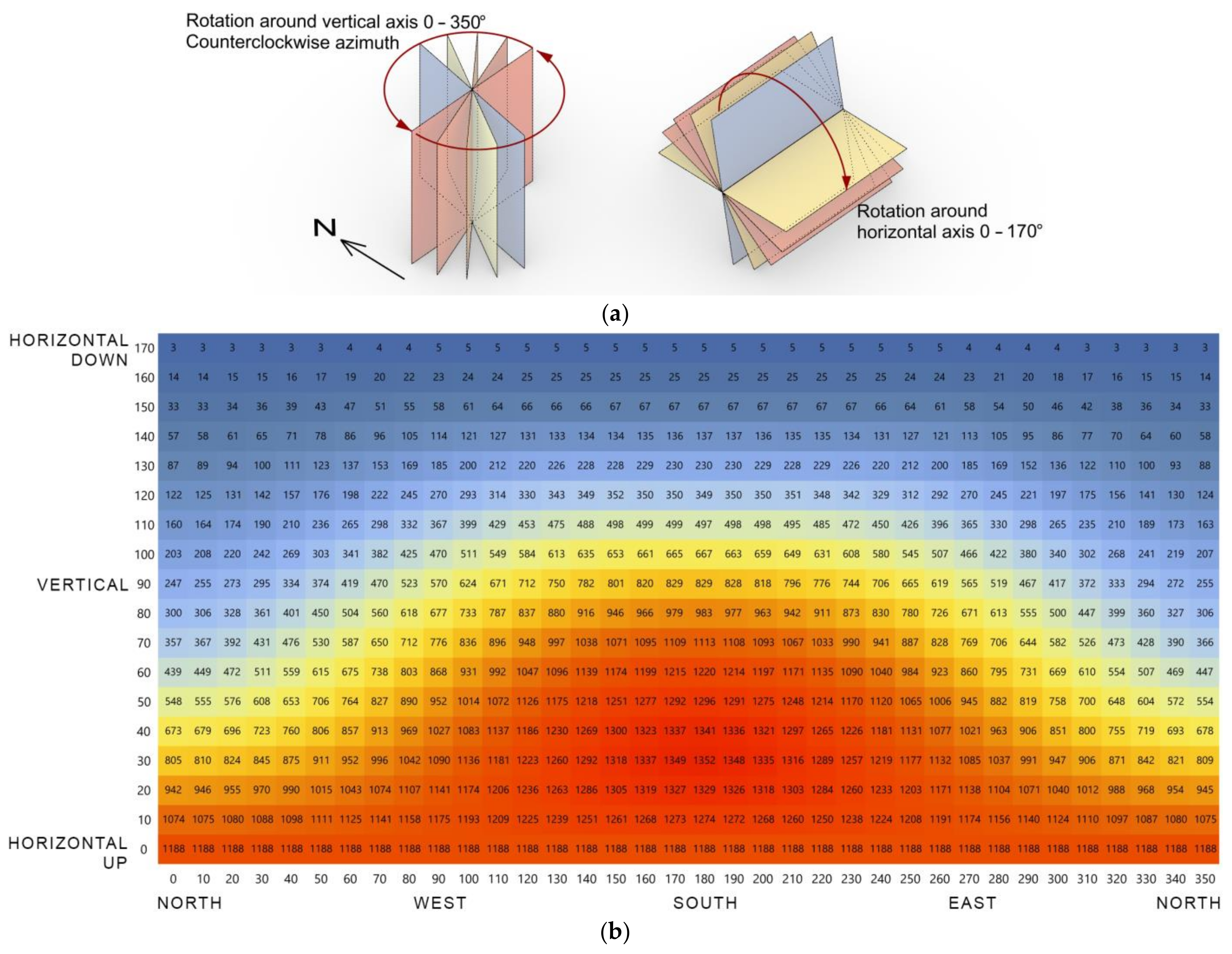
Calculation with Ladybug: the plugin for the analysis of weather data in Grasshopper uses the GenCumulativeSky algorithm [36]. This executable creates a discretised model of the sky dome made of 145 patches based on Tregenza subdivision [37] with specific solar radiation for each patch. The model is based on Perez expressions for sky luminance distribution [36,38]. The algorithm in Ladybug computes the irradiations of cumulative sky patches from direct normal and diffuse horizontal irradiance values, which are measured and recorded via the list, part of the EnergyPlus Weather file—reference year climate data [39,40]. Thus, the cumulative sky model simultaneously includes sky light and beam solar radiation. This model of the cumulative sky is then used as a preprocessor to calculate the radiation of a specifically oriented plane using the following formula, where Eβ [kWhm−2] is the amount of total radiation energy falling on the plane oriented at any spatial angle, γi [rad] is an angle between the normal of this plane and the specific cumulative sky patch i, and Ei [kWhm−2] is the total radiation energy of the specific patch i:
In contrast, the mathematical model by Kittler and Mikler uses significantly less data. This model uses only the reference sky cloud coverage data. The irradiation estimation of the set plane is calculated only from latitude (𝜑), solar constant (E0), Linke’s monthly turbidity coefficients (Tm), and monthly sunlight time (Sm) calculated from sky coverage (part of the EnergyPlus Weather file). The complete calculation has 11 expressions to calculate based on following input data: solar declination, solar altitude, solar azimuth, momentary solar constant dependent on declination, direct irradiance under cloudless conditions (PEbβ), diffuse irradiance under cloudless conditions (dEbβ), and diffuse irradiance under cloudy conditions (dEzβ). This calculation ends with the final expression to calculate the total irradiation of a plane with an arbitrary angle β per time Δh [35]:
Q = (PEbβ × Δh + dEbβ × Δh) × Sm + dEzβ × Δh × (1−Sm) [Whm−2]
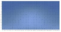
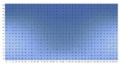
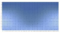
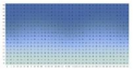
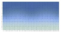
Both techniques can be applied to create the look-up table of every spatial rotation of the plane per specific time interval and for a specific geographic location. The look-up tables of annual irradiation in the solar conditions of Bratislava, Slovakia, were calculated and compared (see Figure 1).


Figure 1.
Look-up tables for annual irradiation [kWhm−2] of every 10° spatial rotation of the plane. (a) Spatial rotation of the abstract plane every 10°. (b) Calculation by Ladybug. (c) calculation using the Kittler and Mikler model. (d) Mean absolute error between these methodologies, MAE = 77.09 [kWhm−2]; the values of the Kittler and Mikler model are lower.
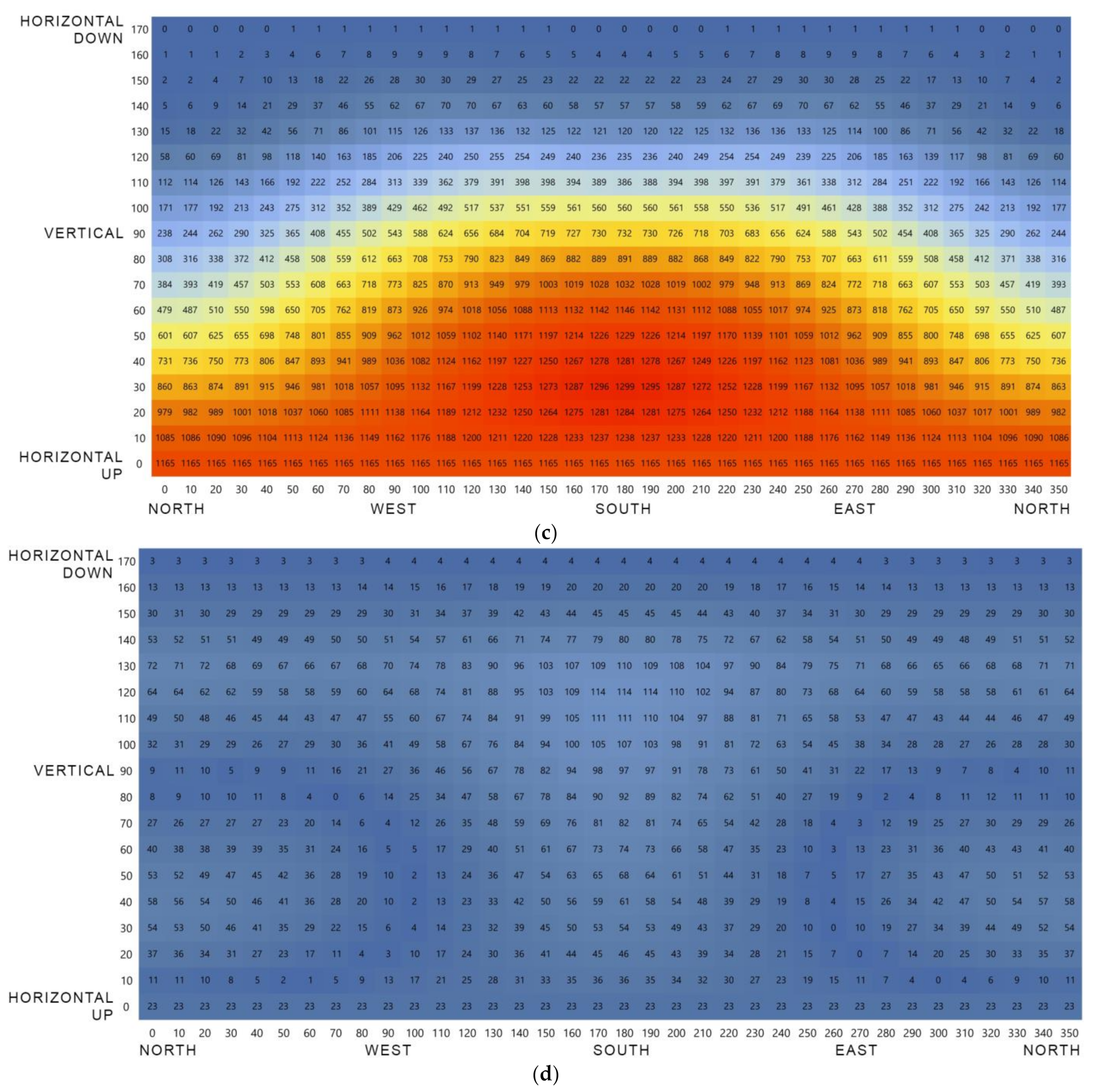
With each mentioned methodology, it is possible to calculate the irradiation of every spatial rotation of the plane per specific time interval in a specific geographic location. The energy gain of the outcome per area for every spatial rotation of the plane E [kWhm−2] divided by its annual maximum Emax [kWhm−2] represents the percentage value of the solar potential Φsol [%] of the orientation of the plane under site-specific conditions.
Φsol = E/Emax × 100 [%]
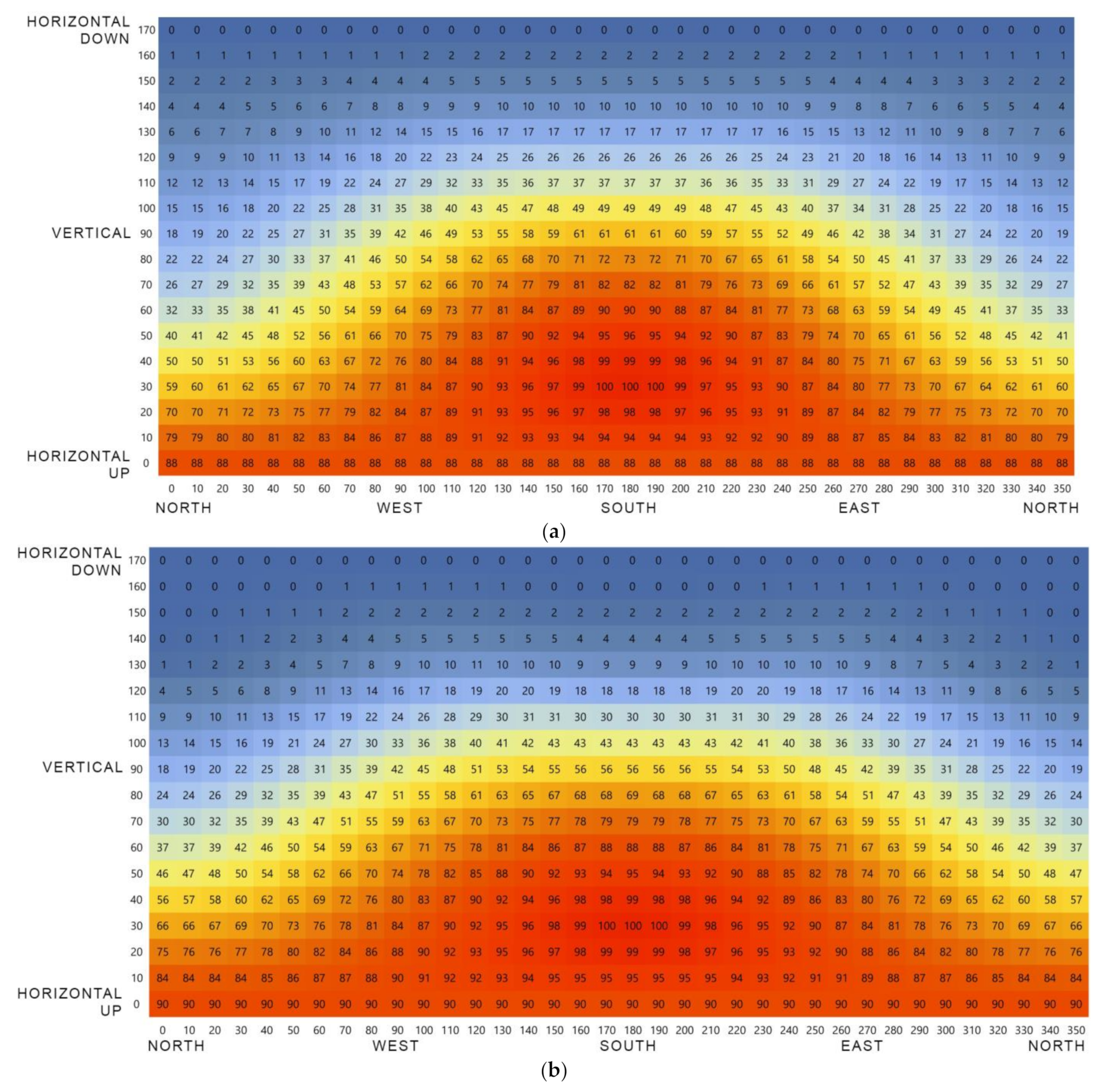
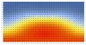
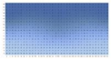
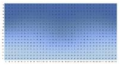
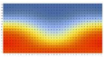
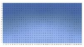
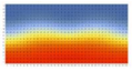
Figure 2 depicts the look-up tables for solar potential of an abstract plane for every 10° of spatial rotation in the solar conditions in Bratislava calculated by Ladybug and Kittler and Mikler’s model. The calculated table is an easy-to-use preprocessor and, using the described methodology, can be generated for any world location and any time interval.

Figure 2.
Solar potential Φsol [%] for every 10° of spatial rotation of an abstract plane in the solar conditions of Bratislava. (a) Calculation with Ladybug. (b) Calculation with the model by Kittler and Mikler.
3.4. Solar-Surface-Area-to-Volume Ratio
With a solar potential look-up table, the solar surface area is calculated as the sum of every side’s surface area As [m2] multiplied by the corresponding solar potential Φsol [%], where s is the index of the side and n is number of geometry sides evaluated.
Solar-surface-area-to-volume ratio, then, defines the size of the solar surface area relative to a specific volume of the object.
4. Algorithm of Solar-Surface-Area-to-Volume Ratio
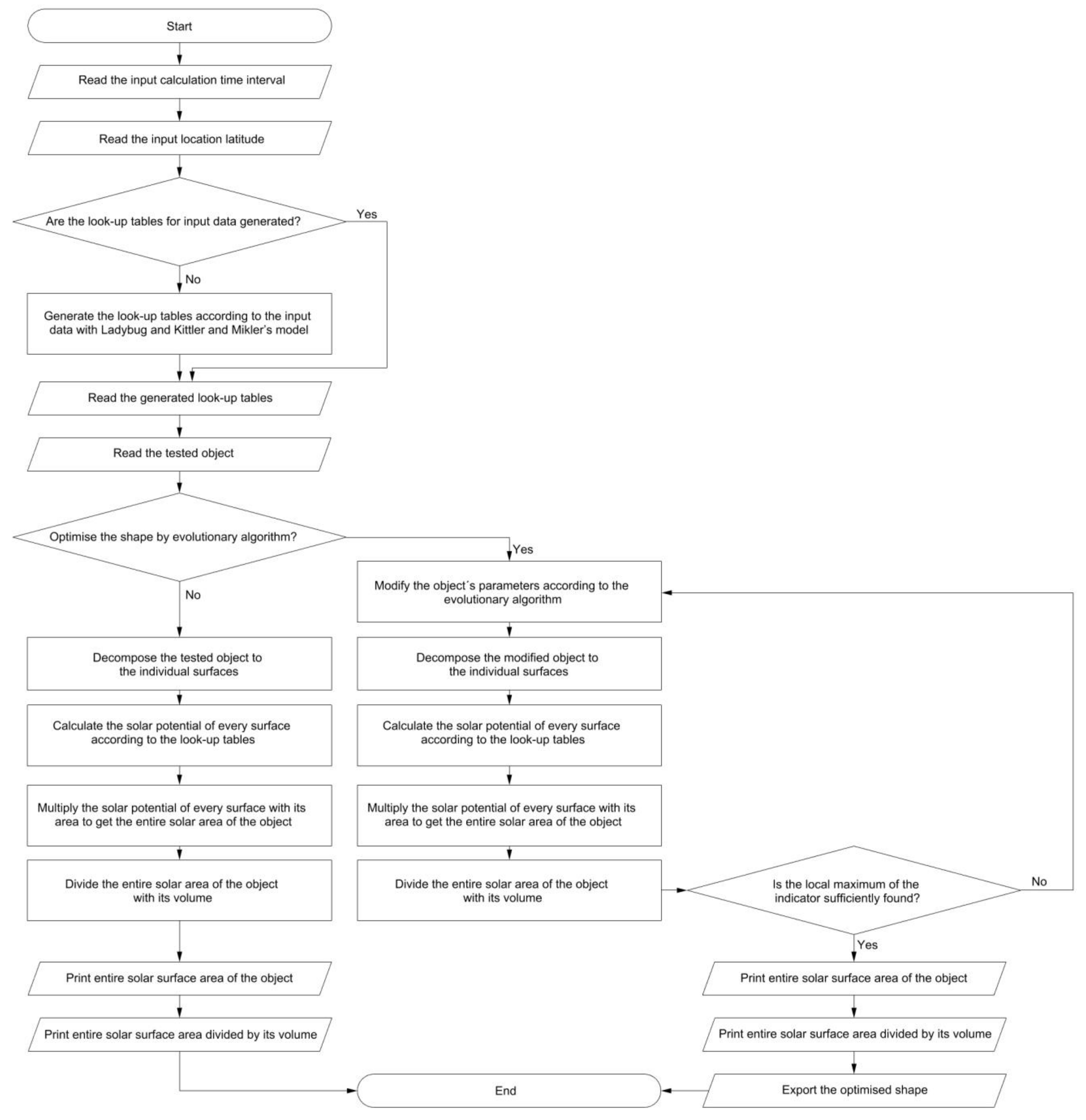
The mentioned methodologies are well-suited for use without computing technology, especially with generated look-up tables. However, the algorithm was also scripted in Grasshopper to make the calculations of shape variations faster, generate the look-up tables for different time intervals and locations, and connect it to the Galapagos evolutionary algorithm [41], used to find ideal shapes and optimise the form. The abovementioned algorithm helps to compare the solar-surface-area-to-volume indicator with surface-area-to-volume ratio and fully explore the possibilities of the indicator’s utilisation. The described methodologies disregard self-shadowing and, thus, they are quick to calculate. The algorithm is composed of the steps depicted in Figure 3.

Figure 3.
The algorithm for solar-surface-area-to-volume ratio. The algorithm without the evolutionary optimisation part was also scripted in Javascript to help the public calculate and visualise the solar surface area and solar-surface-area-to-volume ratio online.
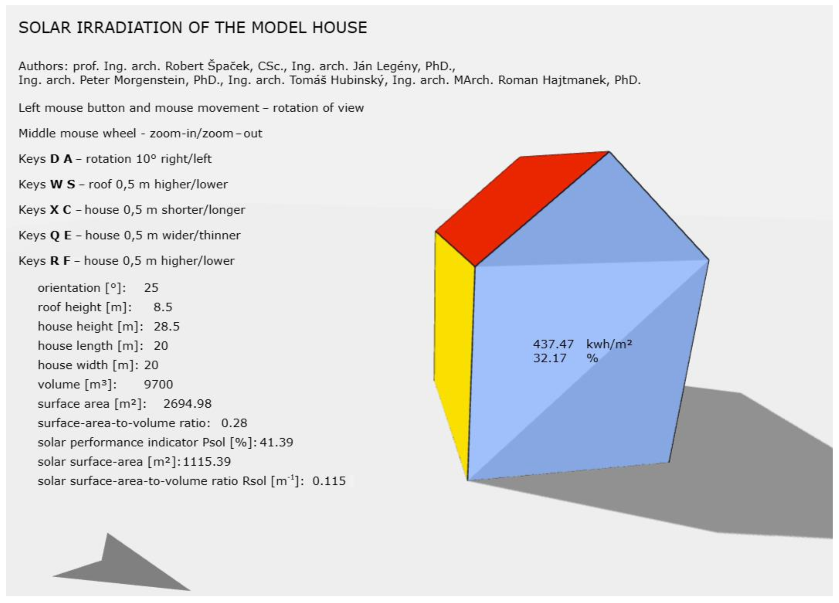
To present the analysis and described indicators to the wider public, an easy-to-use Javascript web application (see Figure 4) was developed and made available at solarmodel.hajtmanek.sk. The user is invited to modify proportions of the 3D building model and is able to see the changes in the solar potential of its faces and mentioned indicators immediately. In this way, public awareness can be expanded, which can result in optimised building shapes for solar gains and increased use of this renewable energy source.

Figure 4.
Web application solarmodel.hajtmanek.sk for visualisation of solar potential and indicators.
5. Evaluation of the Model House under Different Site-Specific Conditions and Time Intervals
To demonstrate the methodologies used, the house model was evaluated under different site-specific conditions provided by three different geographic locations: Bratislava in Europe, San Juan in America, and Wagga Wagga in Australia. The time intervals of analyses were defined for each season and for annual calculation. The Linke coefficients were used according to those found within Worldwide Linke turbidity information [42]. Table 1 shows the look-up tables of solar potential generated for each location with respect to seasons and annual values. The tables were calculated with Kittler and Mikler’s model and compared to Ladybug calculation with mean absolute error.

Table 1.
Generated look-up tables for annual and seasonal solar potential calculated with Mikler and Kittler’s model and their MAE with the Ladybug model. The images within the table provide a visual overview of the calculated values; a file with readable values for each field of the look-up tables can be found online at: https://doi.org/10.6084/m9.figshare.21768332.v1 (accessed on 22 December 2022).
The model of the house was defined as a 20 m long, 20 m wide, and 20 m high building with a pitched roof and rotated 45° off the south–north orientation (see Figure 5 below). The volume of the house was 9000 m3. Every side of the house was numbered. A drawing of the house with its geometry unfolded is in Figure 5.
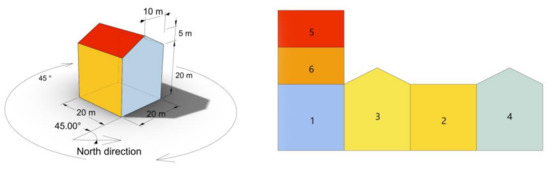
Figure 5.
The model of the house with all dimensions and its geometry unfolded with numbered sides.
The solar potential of the house was determined with the use of look-up tables and every side’s orientation. Subsequently, according to the algorithm, the solar surface area and the solar-surface-area-to-volume ratio of the object were obtained. With the same approach, the annual and seasonal values were calculated (see Table 2).
Table 2.
Calculated values for Bratislava, Wagga Wagga, and San Juan. Annual values are shown for every side of the house. The seasonal values are only applicable with respect to the entire solar surface area and the solar-surface-area-to-volume ratio of the object.
6. Comparison with the Surface-Area-to-Volume Ratio
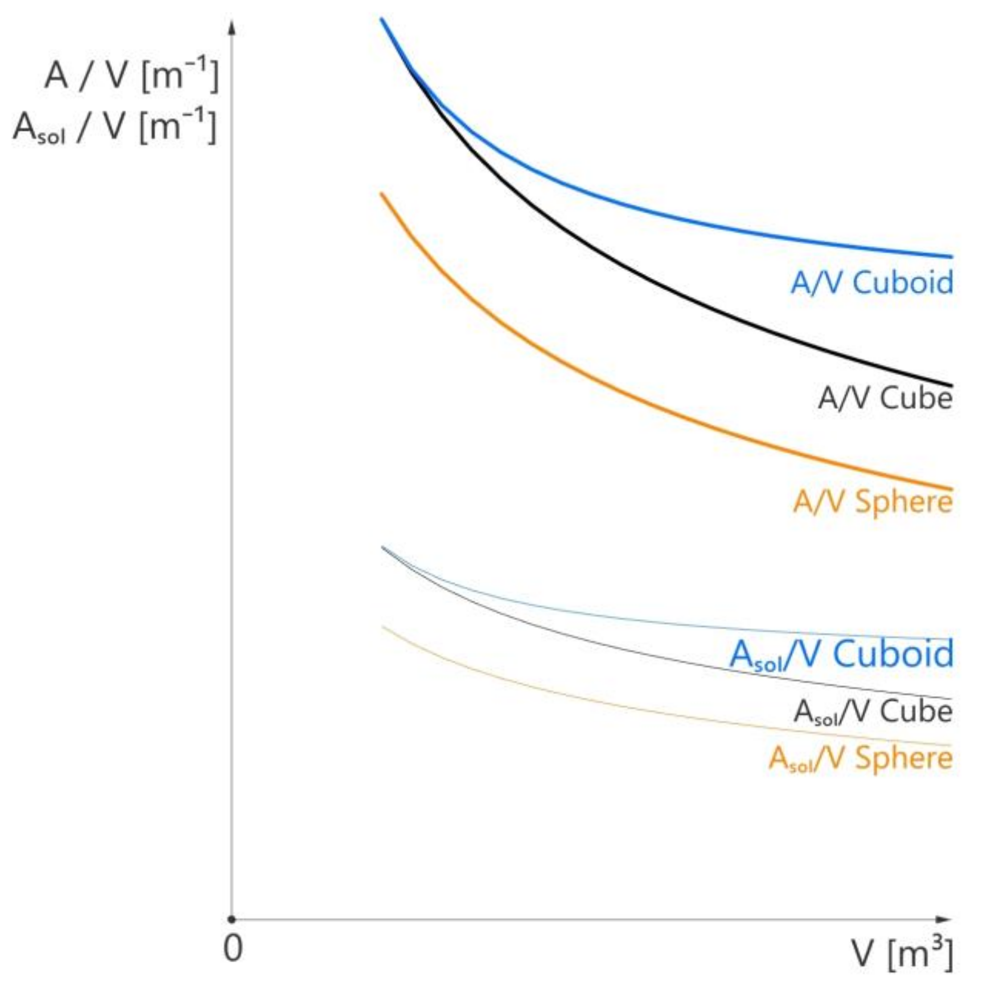
Because the values of the solar-surface-area-to-volume ratio are stated in the same units as those of the surface-area-to-volume ratio, it is possible to compare these two indicators. Figure 6 compares the surface-area-to-volume and solar-surface-area-to-volume ratios of different shapes.
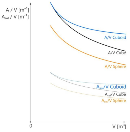
Figure 6.
Surface-area-to-volume and solar-surface-area-to-volume ratios of a sphere, a cube, and a cuboid. The solar surface area is notably related to the entire surface area of the object.
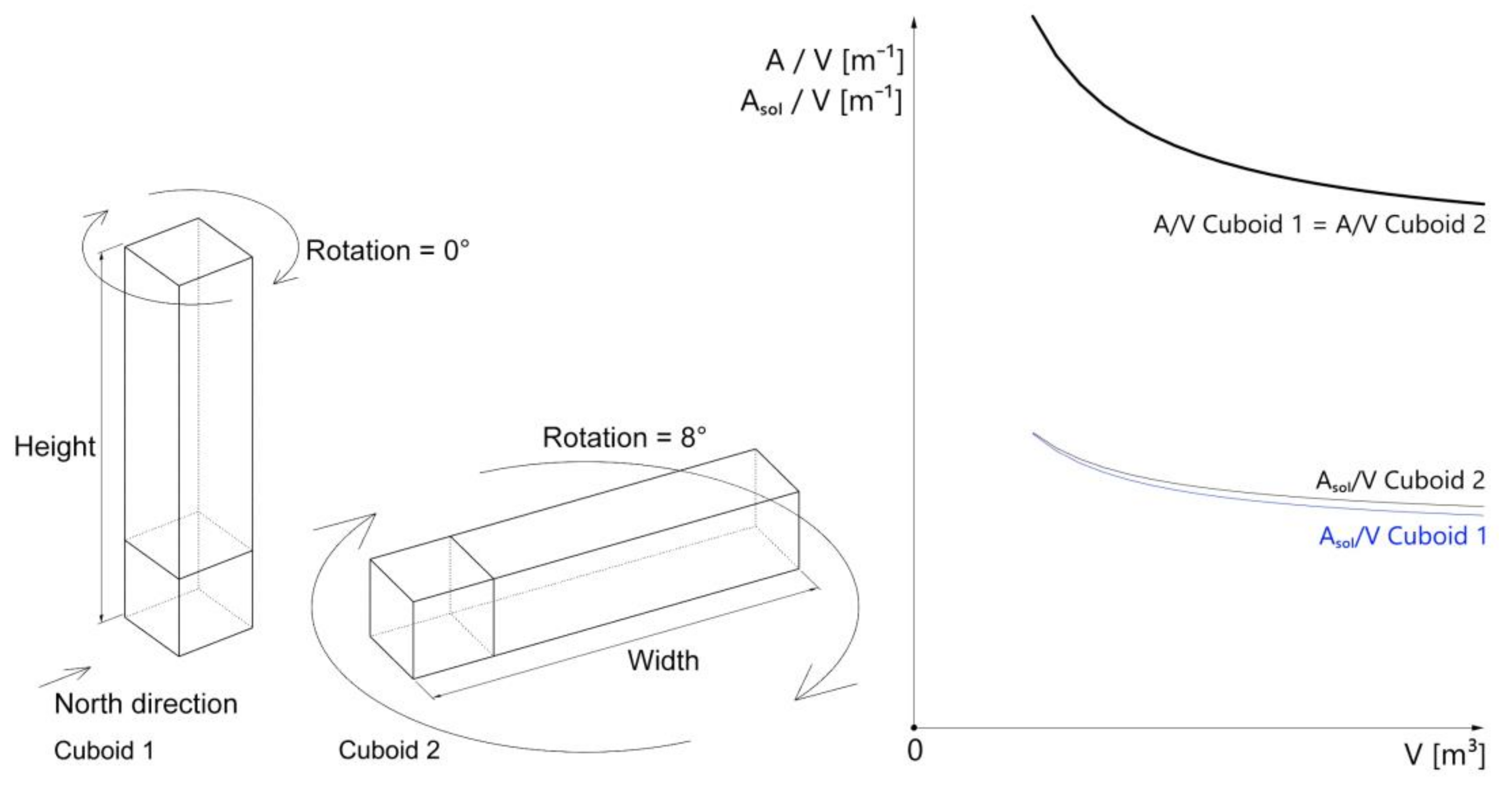
Both indicators depend on the shape of the object, but the solar-surface-area-to-volume ratio also depends on the proportions and orientation of the object, as can be noticed in the different cuboid variations in Figure 7. The orientation, height, and width of the cuboid were designed differently, with the result being identical surface-area-to-volume ratios but different solar-surface-area-to-volume ratios.

Figure 7.
Cuboids designed with variations in height, width, or orientation to the north and their graphs of surface-area-to-volume ratio and solar-surface-area-to-volume ratio.
6.1. Ideal Shape for Solar-Surface-Area-to-Volume Ratio
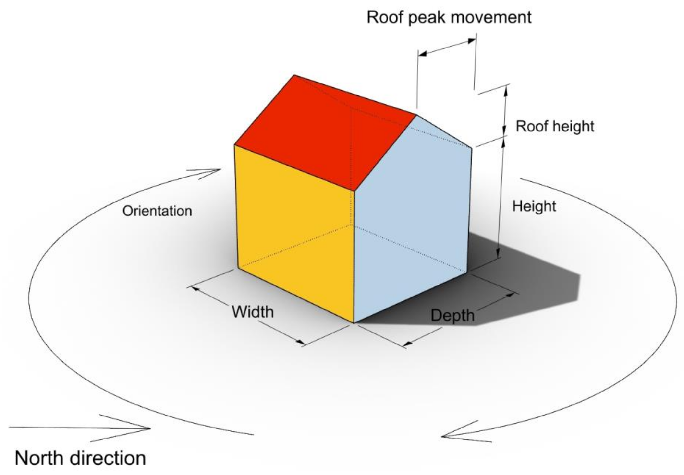
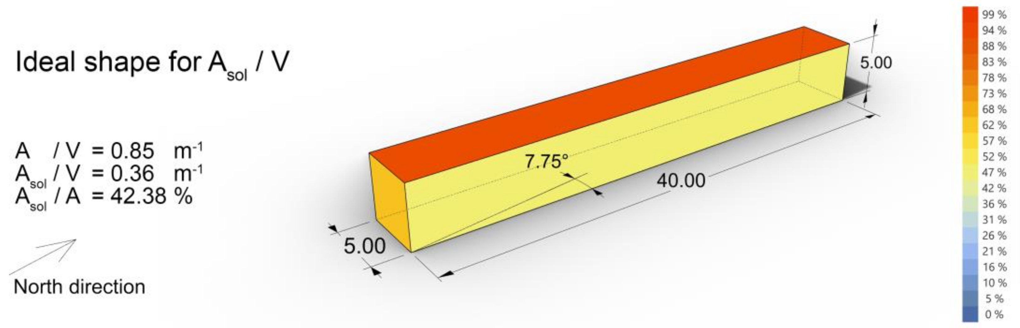
Further research was focused on finding the ideal building shape for solar-surface-area-to-volume ratio for a defined volume, because the use of the indicator will lead the designer to prefer this shape. The form of a building is defined by many parameters. In the course of the research, the authors worked with a simplified building model consisting of the same mass with variable height, width, depth, orientation, inclination, and type of roof with a predefined volume of 1000 m3 (see Figure 8). To simulate the usable form, the width, depth, and height were set to not be less than 5 m. As the building model is defined by many parameters, its ideal shape was sought for using a genetic algorithm that maximizes the solar-surface-area-to-volume ratio. The genetic algorithm was provided by the Galapagos plugin for Grasshopper [41].

Figure 8.
Variable parameters of the model building with constant volume of 1000 m3.
Genetic algorithms are used for optimisation of input variables to find the maximum or minimum of an optimisation objective, which is the outcome of a function with an unknown waveform. The maximum is searched for through generations of variations in the input variables. The algorithms are based on Darwin’s evolution theory and natural selection, as well as Mendeley’s theory of genetic heredity. Such a tool then autonomously searches for new, better solutions in contrast to predefined static normative values.
The solar conditions of Bratislava were used for the search of the ideal shape. This explanatory location of Bratislava was chosen because it is situated in a moderate climate, where the indicator of surface-area-to-volume ratio is widely used for shape evaluation. The result is depicted in Figure 9.

Figure 9.
Ideal shape for solar-surface-area-to-volume ratio.
6.2. Ideal Shape for Both Indicators
The ideal shape, which would have the best properties for coping with both potential losses and potential gains simultaneously, should most appropriately satisfy the requirements of reducing the carbon footprint generated by the manufacture of thermal insulation or active solar systems. To find such an ideal building shape, these two indicators were compared by their division, thus comparing only areas for potential losses A [m2] and potential gains Asol [m2] because, by maximising this value, the outcome shape should be compact—minimising the energy losses and minimising the thermal insulation needed—but also have significant area for generating solar energy:
Psol = (Asol/V)/(A/V) =
= (Asol/V) × (V/A) =
= Asol/A [-]
The outcome shape created by maximising this coefficient was searched for, using the same variable building model with a volume of 1000 m3 under the same solar conditions, by the genetic algorithm (see Figure 10).
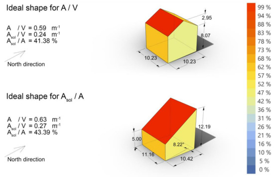
Figure 10.
Top: ideal shape for surface-area-to-volume ratio; bottom: shape optimised simultaneously for both indicators, A/V and Asol/V.
The resulting potential energy coefficient (Psol—Solar Performance Indicator) represents the boundary line between the efficiency of insulation and of active solar systems, thus indicating whether it is reasonable to invest in insulation or rather into active solar systems with respect to their efficiency in order to lower the carbon footprint. Pure maximisation of this value is obviously not representative of the ideal situation for carbon footprint, as both different types of thermal insulation and solar panels with various efficiencies have different carbon footprints. Thus, it would be possible to search for the ideal value of this coefficient, which is neither maximum nor minimum but would generate shapes mostly lowering carbon footprint using various materials by approaching this value. However, this observation is not within the scope of this research, which was further focused on the examination of the correlation between those indicators and energy balances in the physical conditions of a case study of residential buildings in Bratislava.
7. Case Study: Verification of the Solar Performance Indicator on Existing Buildings
To verify the correlation between the Solar Performance Indicator and the measured and calculated energy performance of buildings in practice, a case study was elaborated. Specifically, the case study was intended to compare the measured heating demands of existing buildings as obtained from the heat provider with the calculated energy demands, as well as the potentials in the case of theoretical refurbishment of the buildings envelopes to current standards. These included the principles of integration of renewable energy sources as required by the European Energy Performance Directive [43]. In our case we focused solely on active solar systems situated on surfaces of façades and roofs.
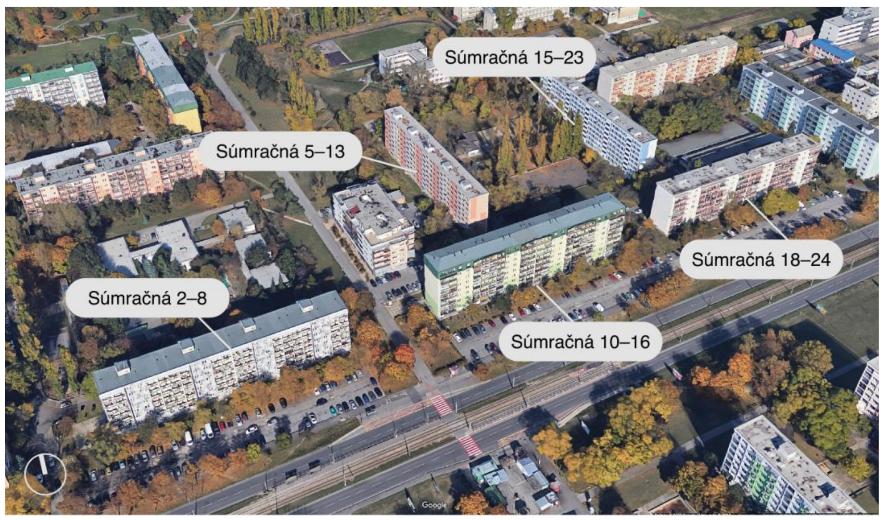
The Ostredky housing estate built in Bratislava in the 1960s consists predominantly of seven–eight-storey monofunctional residential prefabricated slabs with main façades oriented toward east–west or south–north. After the change in the ownership structure from cooperative to individual in the 1990s, the structures gradually underwent individual refurbishment, targeting the thermal parameters of the building envelopes by improving insulation and replacing original windows. For the case study, five buildings were chosen: Súmračná 2–8, Súmračná 10–16, and Súmračná 18–24 with main façades of the slabs orientated towards south–north, and Súmračná 5–13 and Súmračná 15–23 with main façades oriented towards east–west (Figure 11).

Figure 11.
Ostredky housing estate, Bratislava, with marked buildings selected for the case study. Source: Edited by the authors based on CNES/Airbus, European Space Imaging, Maxar Technologies, 2022. Available at: https://www.google.com/maps/@48.1561984,17.1679487,294a,35y,12.52h,45.54t/data=!3m1!1e3 (accessed on 22 December 2022).
7.1. Input Data and Calculation Presets
The goal of the case study was to confirm a correlation between the Solar Performance Indicator values and the overall energy balance of the given residential blocks and, thus, to validate the developed indicators for their practical use. For comparison, the data needed to be systematised and transposed to comparable datasets using an Excel worksheet populated with the input data. The Excel worksheet was structured into five sheets carrying data and calculations related to each of the five buildings, and one additional sheet with an interactive control panel and overview of the results. For each of the five residential buildings, basic parameters were collected in a separate sheet, such as physical dimensions (areas of surfaces—opaque and transparent parts of the building envelopes, volumes, number of storeys) and basic indicators of urban economy (floor area ratio, number of dwellings, etc).
For the heating demands of observed buildings, the input data consisted of their monthly consumption collected by the heat provider for the period from 2009 to 2013 in kWh (the data does not include energy for the preparation of domestic hot water preparation). The measured heating demands per building vary between the years, not only due to changing weather conditions over the years but also because individual buildings have undergone refurbishments as mentioned above. To limit the influence of the refurbishment process on the calculations, we are using the average consumption per annum over the years 2011–2013 (3 years) when the data were rather stabilized. However, due to the wide range of possible factors affecting the real heating demands of selected buildings that are beyond the capacity of this study, the intention was to frame a tendency and show the possible deviations between the calculations and the real measurements.
Within the Excel worksheet, an interactive tool was created for dynamic energy performance calculations, respecting the general principles of specifying energy losses and gains in the central European region. Thermodynamical calculations in the research conducted are based on normative calculation methods for the heating demand of buildings as defined in STN 73 0540 [44], ÖNORM B-8110-6 [45], and EN ISO 13790 [46], respectively, as well as other specialised literature by Chmúrny [47] and by Riccabona [48]:
Qh = (Qt + Qv) − 𝜂 ⋅ (Qs + Qi) [kWh].
The average annual heating demand Qh has been calculated for single buildings by subtracting the sum of the average annual internal gains (Qi) and the passive solar gains through windows (Qs)—both multiplied by the specific gain utilisation factor (𝜂)—from the sum of average annual heat losses through ventilation (Qv) and heat transfer through the building envelope (Qt). For the calculation of the internal gains, an average of 3.75 W/m2 was considered as the mean heat production of persons and devices in residential buildings. The input of solar gains for the heat loss calculation have been reduced accordingly to reflect only the heating season of the year when they can be used. The degree days used in the calculation of energy loss by heat transfer through the building envelope were based on the average number of real degree days of the heating seasons 2011–2013 as indicated by the local heat provider. Furthermore, the calculation of energy loss by heat transfer through the building envelope was calculated in variations. It was based on a dynamic selection of the overall heat transfer coefficients corresponding to the extent of surface types (opaque and transparent façade, roof, and ground). The extent of these surfaces was also dynamically adjustable, resulting in calculation variations.
To allow for the evaluation of the influence of increasing thermal insulation requirements over the course of the years 2013, 2016, and 2021 (National regulations in Slovakia, to be in line with the European Energy Performance of Buildings Directive (EPBD)), a dynamic selection of the overall heat transfer coefficient values for particular structural elements of the building envelope was implemented into the calculation, available in the control panel of the Excel worksheet. By using the minimum required values for heat transfer coefficient, further specification of materials used and their thickness could be avoided in favour of a generally applicable approach.
To calculate the cooling demand in the summer period, a formula adapted according to EN ISO 13790 [46] was used based on the literature by Riccabona [48]:
Qc = fcorr ⋅ (1 − 𝜂s) ⋅ (Qss + Qis) [kWh].
In this calculation, solely the summer season was reflected considering passive solar gains (Qss) and internal gains (Qis). The gain utilisation factor for the summer season (𝜂s) was based on the temperature gradient and resulting degree days during summer. The zoning correction factor (fcorr) was set to a value of 1 for the scope of this study.
The dynamic calculation variations represent the resulting potential energy balances in the case of a theoretical general refurbishment of selected buildings. Therefore, in addition to active solar systems, appropriate shading as well as the influence of heat recovery from ventilation have also been considered in the calculations. The heat recovery option for ventilation can be selected in the control panel sheet.
To visualise the overall energy consumption of buildings, the calculation of hot water demand and electricity use based on daily consumption values per dwelling unit has been adopted from previous research [49].
For the determination of solar potential, the available surfaces of the building envelopes were examined. Solar irradiation of façades and roofs was determined by simulation using the cumulative sky tool provided by the Ladybug plugin in Grasshopper as described above.
As the window coverage of the façades varies from 18% to 30% in the selected buildings (and the short façades have no windows at all), for the scope of the study, it was predetermined that each of the façades will be covered by 35% with photovoltaics (PV) and 20% with solar thermal panels (ST). The roof surfaces were covered with 60% PV and 15% ST. Based on previous research, the overall system efficiencies were pre-set as 15% for PV and 25% for ST [49].
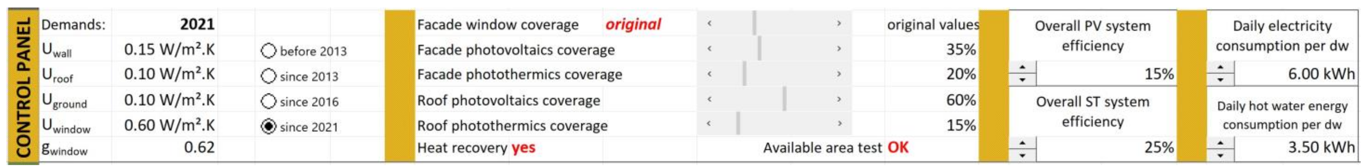
The input parameters can be varied using the control panel of the Excel worksheet (Figure 12), enabling the alteration of U-values for the overall heat transfer coefficients, façade window coverage ratio (selectable between realistic values of the building and an average percentual value), active solar system coverage of roofs and façades and their efficiency values, as well as the daily consumption rates of electricity and hot water per dwelling unit. The heat recovery option can also be switched.

Figure 12.
Overview of the Excel calculation sheet control panel with the pre-set values.
7.2. Calculation Results
Results of the calculation are shown in the tables below (and are available in the Excel Evaluation sheet as well). Table 3 focuses on the basic verification of the calculation by comparing the measured average annual heating demands of buildings in the three consecutive years 2011–2013 with the calculated energy demands. The parameters of the building envelope used in the calculation correspond to the standards of the heat transfer coefficient before 2013, and the buildings do not have ventilation heat recovery. The calculation results per square meter of floor area are close to the measured values with the exception of two buildings—Súmračná 2–8 and Súmračná 15–23—where energy efficiency refurbishment has not yet been implemented. It can be noted that this result verifies the coherence between the calculation method and the measurement; thus, the calculation can be further used for exploring theoretical development scenarios of the case study.
Table 3.
Comparison of the measured annual average heating energy demands during years 2011–2013 and the calculated energy demands of five residential buildings in the Ostredky housing estate, Bratislava. The parameters of the building envelope used in the calculation correspond to the standards of the heat transfer coefficient before 2013 with no ventilation heat recovery. Two columns on the right show the difference between measurement and calculation per m2 of floor area; notable differences are in case of Súmračná 2–8 and Súmračná 15–23, where basic refurbishment has not yet been completed.
The scope of further calculations was to simulate a scenario where the energy performance of the selected existing residential buildings is highly improved (deep renovation for energy performance purposes) to correspond to the demands of Nearly Zero Energy Buildings (NZEB) as defined by the revised European Energy Performance of Buildings Directive (EPBD): “‘nearly zero-energy building’ means a building that has a very high energy performance (…). The nearly zero or very low amount of energy required should be covered to a very significant extent by energy from renewable sources, including energy from renewable sources produced on-site or nearby”. [43] The theoretical deep renovation of the observed buildings scenario introduces the integration of renewable energy sources—active solar systems (photovoltaic panels and solar thermal panels)—into the building envelope to the extent mentioned above. The thermal properties of the building envelope were gradually increased by the National Slovak Standardisation (STN 73 0540 and its amendments) to the standards of NZEB as required by the European Union [43] (see Table 4). Furthermore, the deep renovation in this case study includes a heat recovery system for building ventilation (the efficiency of heat recovery in the calculations is 0.8).
Table 4.
Difference between minimal required values of heat transfer before 2013 and since 2021 corresponding to the Nearly Zero Energy Buildings concept implemented in Slovakia by the National Standardisation STN 73 0540.
The results of the calculation of the deep renovation scenario are shown in Table 5 below. The introduced improvements in the thermal properties of the building envelope as well as the reduction in heat losses through ventilation by heat recovery enabled a considerable increase in the energy efficiency of the observed buildings. Integration of active solar systems in the façades and roofs resulted in on-site generation of energy from renewable sources which almost covered the total energy demands including hot water, cooling, and electricity of the buildings Súmračná 2–8, Súmračná 10–16, and Súmračná 18–24, and even exceeds the total energy demands of Súmračná 5–13 and Súmračná 15–23.
Table 5.
Overview of the calculated energy demands and potentials of five residential buildings in the Ostredky housing estate, Bratislava in the event of a deep renovation. The calculated overall energy balance shows the coverage of more than 90% of the energy needs of Súmračná 2–8, Súmračná 10–16, and Súmračná 18–24, and exceeds the total energy demands of buildings Súmračná 5–13 and Súmračná 15–23.
Because the buildings examined have different orientations and also vary in dimensions and basic parameters, the calculation results per unit of floor area as provided in Table 6 offer a better comparison of the energy performance of the buildings. Moreover, finally, the correlation of the calculated energy performance of singular buildings and their solar performance indicator (Psol), solar-surface-area-to-volume ratio (Rsol), and solar surface area (Asol), as well as the widely used surface-to-volume ratio, can be assessed.
Table 6.
An overview of the calculated energy demands and potentials related to floor area in the case of a deep renovation of five residential buildings in the Ostredky housing estate, Bratislava, provides a direct comparison of the energy performance of buildings. In addition, the table shows the values of the easy-to-use building solar potential indicators proposed by the authors and their relationship to the calculated energy performance of the buildings.
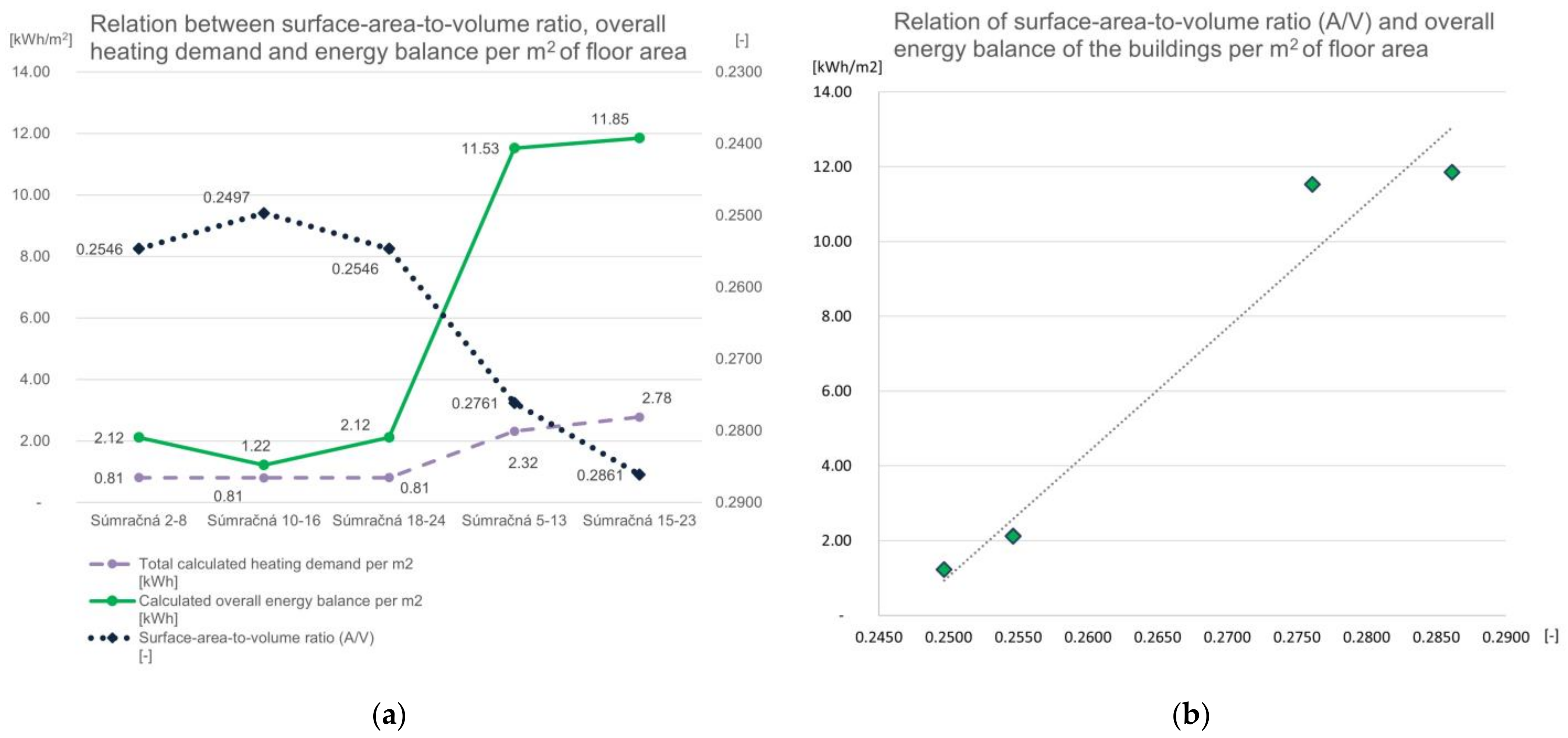
From Table 6, it is obvious that the calculated heating demand per square meter of floor area and the widely used surface-to-volume ratio correlate. However, as Figure 13 and the calculation in the Excel worksheet show, the differences in heating demand between buildings tend to be less pronounced when the buildings are well insulated and the heat recovery for ventilation is engaged. Despite the fact that the surface-to-volume indicator is an easy-to-use tool for the initial phases of building design, its applicability with increasing insulation standards, the introduction of advanced ventilation systems, and integration of active energy-collecting systems gradually drops. The irrelevance of the surface-to-volume ratio for the overall energy balance of the examined buildings is shown in Figure 13, where the surface-to-volume ratio has better values for buildings with lower overall energy balance per square meter and vice versa.

Figure 13.
The relationship between surface-area-to-volume ratio (A/V), overall heating demand, and energy balance per m2 of floor area. (a) The chart plotted with values on y-axis shows that, while the calculated heating demand corresponds to the A/V (the lower the A/V value, the lower the heating demand), the overall energy balance (which includes active energy gains) does not; (b) Relation of surface-area-to-volume ratio (A/V) and overall energy balance of the buildings per m2 of floor area plotted on x-axis and y-axis shows that A/V correlates with values of overall energy balance, but inversely—higher (worse) A/V values correspond to better energy balance.
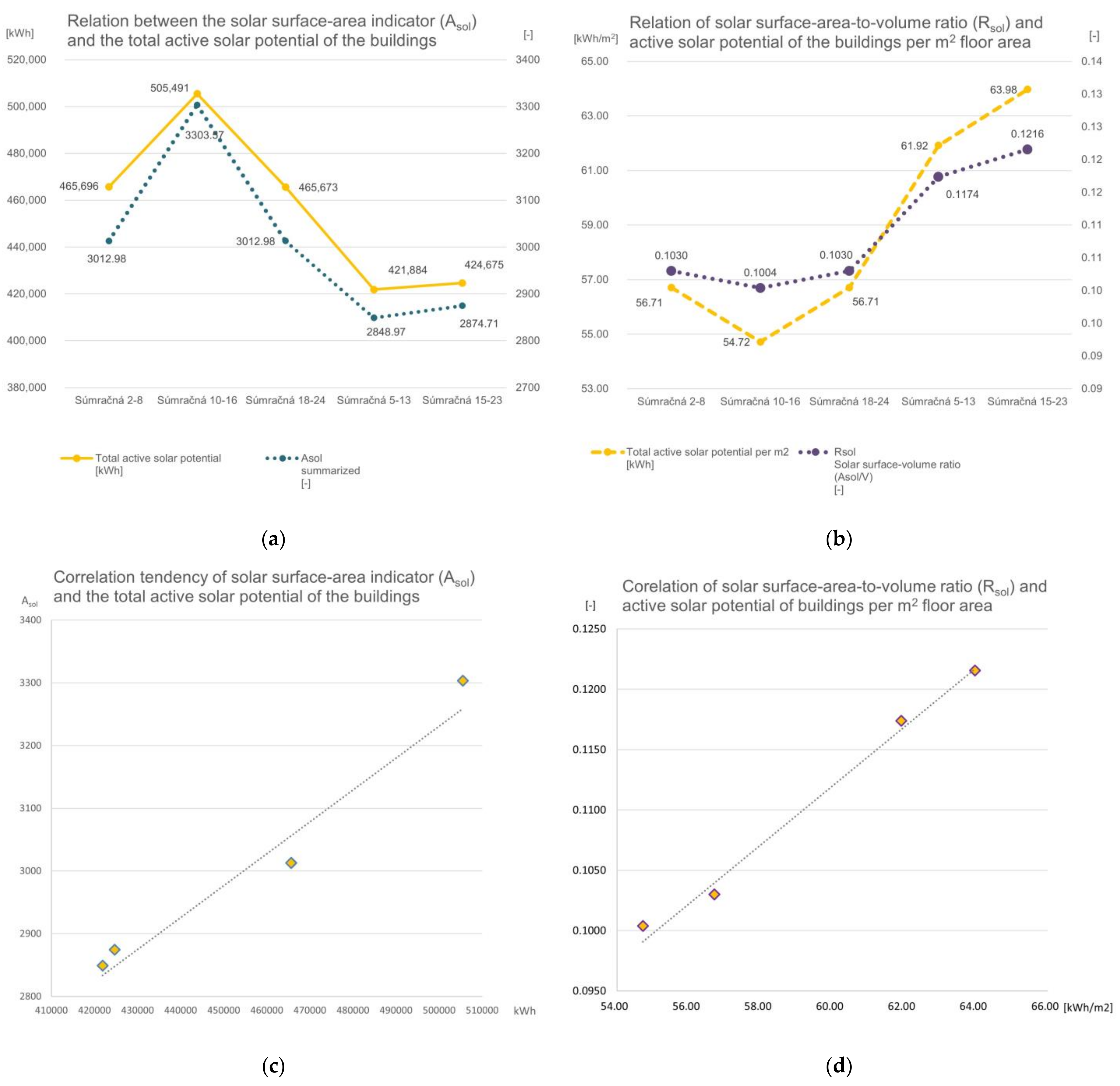
The solar surface area indicator (Asol) correlates with the calculated total active solar potential of the building, and can thus be used for the basic assessment of the overall solar energy potential of the building in the early design phases, as shown in Table 6 and depicted in Figure 14a.
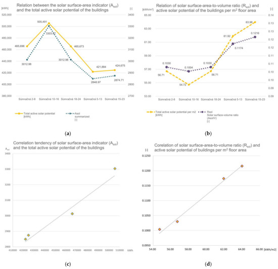
Figure 14.
Four graphs visualising the calculation results shown in Table 6 and focusing on the relation between particular energy performance values and proposed indicators: (a) Confirmed correlation between the solar surface area indicator (Asol) and the total active solar potential of the buildings; (b) The chart confirms that solar-surface-area-to-volume ratio (Rsol) and the active solar potential of the particular buildings per m2 floor area correlate; (c) Correlation of solar surface area indicator (Asol) and the total active solar potential of the buildings plotted on x-axis and y-axis; (d) Correlation of solar-surface-area-to-volume ratio (Rsol) and active solar potential of buildings per square meter of floor area. The correlation confirms the applicability of these indicators as tools for quick assessment of the solar performance of buildings under given conditions.
When the solar-surface-related indicator is put into context with the volume or floor area of the building (e.g., Rsol), it is related to the building performance per square meter, such as in the column Calculated overall energy balance per m2 floor area in Table 6 and Figure 14b. Charts in Figure 14c,d confirm the correlation of both Asol to the total solar potential and Rsol to the solar potential per square meter of floor area of the buildings, respectively.
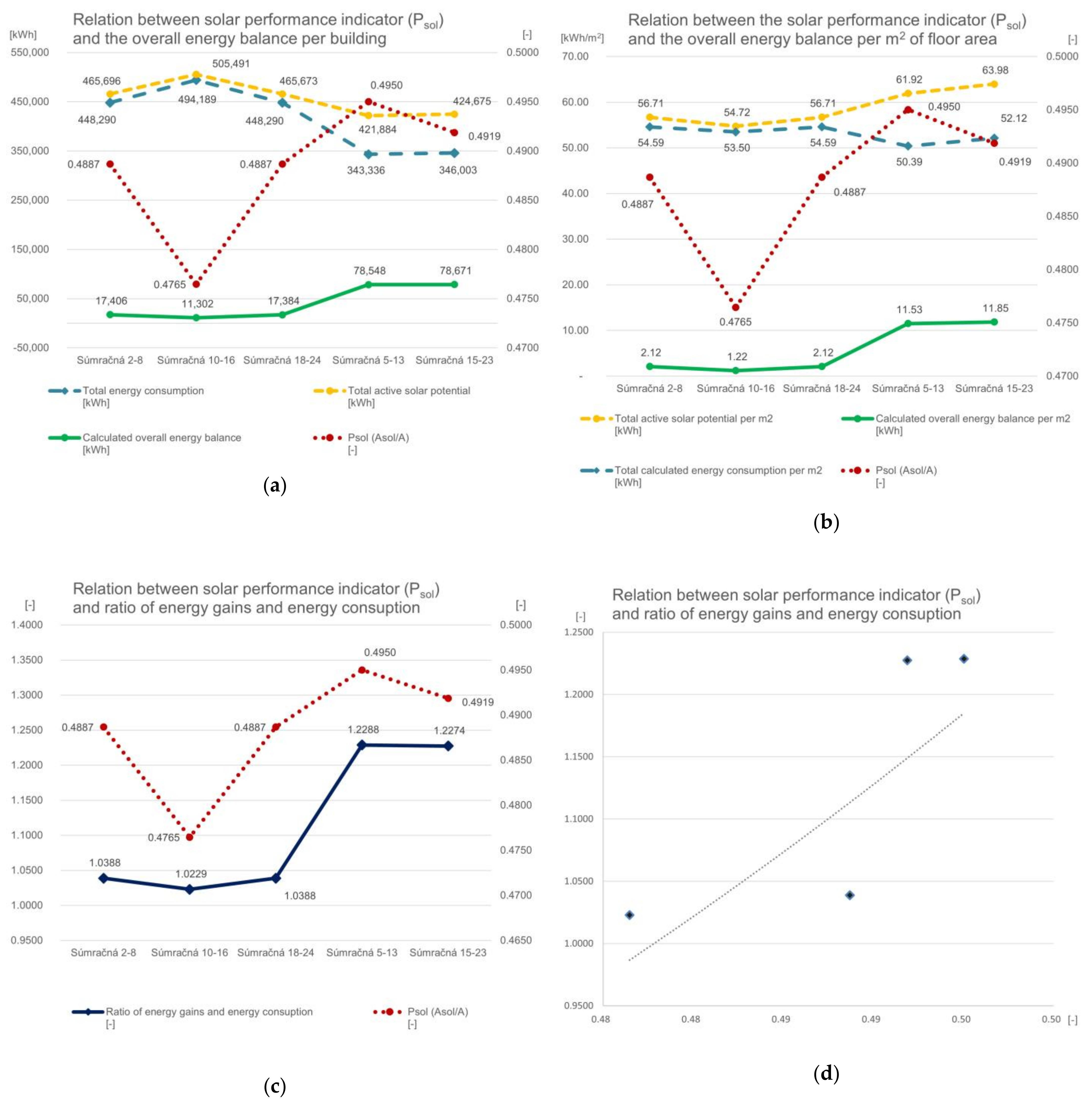
Specifically, the overall cumulative energy balance (in total and per square meter) of a particular building shown in Figure 15a,b corresponds to the solar performance indicator (Psol), thus confirming the possibility of using this simplified method for the assessment of the overall energy performance of a building already in the initial phases of the design process. Furthermore, the relationship between Psol and the ratio of energy gains and energy consumption has been examined, and is shown in Figure 15c,d. The chart shows a correlation between these values, which supports the applicability of the solar performance indicator in a quick comparison of different building shapes in initial design phases.

Figure 15.
Graphs visualising the calculation results shown in Table 6 and focusing on the relation between particular energy performance values and proposed indicators: (a) The chart depicts the correlation of the solar performance indicator (Psol) and the overall energy balance of the building, although, as expected, both the cumulative values of energy consumption and active solar potential are opposed to this indicator; (b) Correlation of the solar performance indicator (Psol) proposed by the authors and the overall energy performance of the building per square meter of floor area. The relationship between Psol and the ratio of energy gains and energy consumption in the chart shows the correlation between these values. The relation between the parameters is shown alternatively plotted (c) on two scales of the y-axis and (d) correlating values plotted on x- and y-axes. The results confirm the possible applicability of the indicator under defined conditions for preassessment of building performance by architects and planners in early design stages.
8. Discussion
The solar-surface-area-to-volume ratio was introduced and defined to evaluate potential solar energy gains. Its calculation is based on the look-up tables related to surface orientation and energy gain as a preprocessor calculated by Ladybug or Kittler and Mikler’s model. The differences between these two techniques may occur because of the low-resolution sky used in Ladybug’s model (only 145 patches) and the dependence on variable sky coverage and Linke’s turbidity factor used in the model by Kittler and Mikler. The difference was insignificant, with a mean absolute error of 77.09 [kWhm−2], which is only 5.68% of the maximum solar energy gain in the conditions in Slovakia.
To demonstrate the whole process of using the introduced indicator, the calculation with the explanatory model house in varied site-specific conditions and seasons was described. The house had differences in solar-surface-area-to-volume ratio during the seasons because the solar energy gain also differs during these time periods. However, the annual indicator was similar, 0.11–0.12, because it is calculated with respect to the maximum solar energy gain in the specific country.
Further research explored the solar-surface-area-to-volume ratio of different geometrical shapes under the conditions of moderate climate (located in Bratislava) rather than exploring different conditions of various locations to compare it with the surface-area-to-volume ratio.
For both indicators (solar-surface-area-to-volume ratio and surface-area-to-volume ratio), ideal building shapes with a volume of 1000 m3 were found with the genetic algorithm, resulting in significant energy performance differences. It was obvious that if the solar-surface-area-to-volume ratio was given preference, it led to an increase in potential losses with the increasing surface area of the object and vice versa (see Figure 9 and Figure 10).
To find the balance between those opposing indicators, the solar performance indicator (Psol) was introduced. Based on this coefficient, the optimal shape was found (Figure 10). Compared to the ideal building shape defined by the surface-area-to-volume ratio (A/V), this new optimised shape scores just 0.04 m−1 worse than the ideal shape for the surface-area-to-volume ratio. When the solar performance indicator was compared to the ideal shape for the solar-surface-area-to-volume indicator (Asol/V), the optimised building shape scores just 0.09 m−1 worse. Using the reverse process:
we can obtain the annual solar energy gain of the building. The annual solar energy gain of the ideal shape for surface-area-to-volume ratio was only 332 MWh and for the solar-surface-area-to-volume ratio it was 425 MWh, which is a 28% improvement. The annual solar energy gain of the ideal shape for both indicators was 374 MWh, which is better by 13% than the ideal shape for the surface-area-to-volume ratio. This analysis of the results confirms an improvement of the energy performance of a given structure when adhering to the proposed indicator.
E = Asol × Emax [kWh]
With respect to the surface-area-to-volume ratio, the ideal geometrical shape is the most compact form possible under the defined conditions. This shape can be applied to minimise energy losses, but it does not take into consideration any potential energy gains. In this case, the resources for thermal insulation of the building are saved, but the potential energy gains are not exploited fully. In contrast, the ideal building shape defined by the solar-surface-area-to-volume ratio optimizes its surface for maximal solar gains, but it is not compact, resulting in greater thermal energy losses through the building envelope. In this case, sufficient solar energy gains can be achieved, but more resources will be spent on thermal insulation. A geometric shape optimised simultaneously for solar energy gains and thermal energy losses at the same time should provide the optimum solution between the two extremes. The building shape is compact, but it also has sufficient solar-active surfaces.
The verification of the indicators proposed by the authors was further examined within the case study with the aim of confirming the correlation of these indicators and the calculated energy performance of real buildings. The results visualised in the graphs in Figure 14a–d confirmed the correlation of the solar surface area indicator (Asol) and the active solar potential of the buildings, as well as the correlation of solar-surface-area-to-volume ratio (Rsol) and the active solar potential of the building per m2 floor area. Such alignment of the results confirms the possibility of predicting the solar potential of a realistic building shape by using the proposed solar energy related indicators Asol and Rsol. Furthermore, Figure 15a,b shows the correlation tendency between the solar performance indicator (Psol) and the overall energy balance of the given structure, and Figure 15c,d shows the relation between Psol and the ratio of energy gains and energy consumption. This, under defined conditions, can be interpreted as a confirmation of applicability of the proposed indicator Psol which combines the demand for compactness of the building form and its energy performance. It needs to be stated that, while the indicator can prove useful in mild climates where minimisation of energy loss through the building envelope is needed, in hot climates, the principle of building compactness can be disadvantageous regarding the natural cooling and shading of the structure. Thus, the Psol indicator needs to be further examined reflecting different conditions. Likewise, the applicability of Asol and Rsol in different conditions should be verified by further case studies, although—as both indicators focus on solar potential—they can be expected to be more versatile under diverse conditions.
There are many factors that affect the overall energy balance of buildings, of which one of the main factors is user behaviour, which cannot be predicted. However, the introduced indicators focus on improving architects’ and urban planners’ decisions in estimating the energy performance of buildings in the context of the implementation of high energy efficiency demands and decarbonisation strategies for the building sector in the initial phases of design. Although the widely used surface-to-volume ratio today serves well in the case of basic predictions of energy losses by heat transition through the building envelope, the proposed solar performance indicator (Psol) additionally incorporates the potential of the building to utilise active and passive solar systems, while at the same time considering energy losses, too. This can also be deduced from the graphs in Figure 14c,d where neither the active solar potential nor the overall energy consumption solely correspond to the Psol indicator, but the combination of both is expressed in the calculated overall energy balance. The indicator can be useful in the basic decision-making process and supports the demand for the integration of energy sources directly on-site.
The solar surface area of a building is usually affected by shading from surrounding structures or other kinds of obstructions. However, when defining the solar performance indicator, we deliberately did not include the parameter of overshadowing of buildings, as the indicator and needed input data would become too complex for its quick use. Advanced tools for estimation of the influence of shading can be used in further design phases. The aim of this tool is also not to affect selection of building materials, definition of building structure, and building elements, which all play a crucial role in determining and lowering the building carbon footprint within its lifecycle.
Furthermore, the case study was focused on calculation of energy consumption and potential characteristics of residential buildings in Bratislava, and for a wider implementation of the indicators it would be necessary to validate the results for diverse building typologies (office buildings, schools, etc.). To verify the applicability of the indicators for other regions, further case studies need to be conducted in different latitudes and under different climate conditions. It can be assumed that, in warmer conditions, the Psol indicator would require modifications; depending on the location, observation of energy loss through the building envelope does not need to be a priority when estimating building energy performance. Contrarily, e.g., where overheating of buildings is the main issue, a loose building shape can perform better.
9. Conclusions
The aim of the research is to highlight the fact that focusing solely on optimisation of form compactness or on solar gains leads to suboptimal results and higher spending on solar active systems or thermal insulation. Optimisation of both parameters in respect of the mentioned solar performance indicator (Psol) represents the balance needed when considering building shapes in the conditions of Central Europe. Despite the simplification of the calculation, it points out the needed balance, and is easy to use. Future research will focus on verification of indicators with different building typologies. Furthermore, the difference between the potential energy gains and losses will be explored, with the aim of adjusting this coefficient in the context of optimisation of the relation between thermal insulation amount, active solar systems, and the connected carbon footprint.
In comparison to the abovementioned Pokorny’s projects’ grading factor (Entwurfsgütezahl), the introduced indicators Asol, Rsol, and Psol calculate not only with the solar active area of south façades but with the entire active solar area of the object, and thus, they are valid also for the locations near The Equator, or in the Southern Hemisphere where the roof or north façade are mostly significant. Above that, calculation with the entire solar surface area of the building’s geometry motivates one to install active solar systems on every side of the geometry with relevant solar energy gains.
The methodology used in those applications ignores the shadowing from the surroundings, because it should be easy to calculate for the wide public, even without the computing technology. However, the online application can be widely expanded—e.g., by adding the shadows calculation with a discrete model of the sky, similar to the Ladybug plugin. It is possible to calculate the discrete sky model with the model by Kittler and Mikler and compare it with the one calculated with Ladybug. The calculation methodology would then also be applicable to the evaluation of public spaces and neighbourhoods. The online models of buildings created could be downloaded and screenshotted by built-in tools. The parameters of downloaded outcomes could be saved to create a new tool that will optimise the physical parameters and offer the building shapes favoured by users.
The simple usability of these tools and indicators by the wide public leads to better energy solutions for buildings and a decrease in CO2 production upon their construction. The next step would be to implement those indicators in the legislation in a way similar to the way the surface-area-to-volume ratio is already implemented.
In architectural practice, the shape of the building is determined by many other conditions in addition to energy optimisation and carbon footprint. These aspects are often evaluated ex post. Familiarising the public with relevant information and making evaluation tools more accessible can lead to a more climate-friendly environment.
Author Contributions
Conceptualisation, R.Š., P.M., R.H., T.H. and J.L.; methodology, R.H. and P.M.; software, R.H. and P.M.; validation, T.H.; formal analysis, T.H.; investigation, P.M. and R.H.; resources, R.H.; data curation, P.M. and R.H.; writing—original draft preparation, R.H., P.M., T.H. and J.L.; writing—review and editing, R.Š.; visualisation, R.H. and P.M.; supervision, R.Š.; project administration, P.M.; funding acquisition, P.M. and J.L. All authors have read and agreed to the published version of the manuscript.
Funding
This work was supported by the Slovak Research and Development Agency, grant number APVV-18-0044 [“Solárny potenciál urbanizovaných území a jeho využitie v koncepte Smart City”/“Solar potential in urban areas and its application to the Smart City concept”] and Culture and Education Agency of the Ministry of Education, Science, Research and Sport of the Slovak Republic (KEGA), grant number 031STU-4/2022 [“More-dimensional model—educative and creative tool in the form of mixed reality for architects and urban planners”/“Viacdimenzionálny model—edukačno-tvorivý nástroj vo forme zmiešanej reality pre architektov a urbanistov”] and Operational Program Integrated Infrastructure co-financed by the European Regional Development Fund, grant number 313021BXZ1 [“Support of research activities of Excellence laboratories STU in Bratislava”].
Data Availability Statement
The solar irradiation of the model house web application for visualisation of solar potential and indicators developed within this research is publicly available at: solarmodel.hajtmanek.sk. The data on energy performance of buildings and related indicators presented within the case study, Ostredky, are openly available in FigShare [50].
Conflicts of Interest
The authors declare no conflict of interest.
References
- Climate and Environmental Emergency—Thursday. 28 November 2019. Available online: https://www.europarl.europa.eu/doceo/document/TA-9-2019-0078_EN.html (accessed on 19 December 2022).
- What Is Carbon Neutrality and How Can It Be Achieved by 2050?|News|European Parliament. Available online: https://www.europarl.europa.eu/news/en/headlines/society/20190926STO62270/what-is-carbon-neutrality-and-how-can-it-be-achieved-by-2050 (accessed on 19 December 2022).
- Potenciál Budov v Znižovaní Emisií Uhlíka je Veľký. SKGBC. Available online: https://skgbc.eu/portal/potencial-budov-v-znizovani-emisii-uhlika-je-velky/ (accessed on 19 December 2022).
- Gupta, V. Thermal Efficiency of Building Clusters: An Index for Non-Air-Conditioned Buildings in Hot Climates. In Energy and Urban Built Form; Elsevier: Amsterdam, The Netherlands, 1987; pp. 133–145. ISBN 978-0-408-00891-4. [Google Scholar]
- Mahdavi, A.; Brahme, R.; Mathew, P. The “LEK”—Concept and Its Applicability for the Energy Analysis of Commercial Buildings. Build. Environ. 1996, 31, 409–415. [Google Scholar] [CrossRef]
- Gurtekin, A.; Mahdavi, A. Performance-Guided Explorations in the Thermal Design Space. In Research in Building Physics Proceedings of the Second International Conference on Building Physics, Leuven, Belgium, 14–18 September 2003; Carmeliet, J., Hens, H.S.L.C., Vermeir, G., Eds.; CRC Press: Boca Raton, FL, USA, 2020; ISBN 978-1-00-010814-9. [Google Scholar]
- Markus, T.A.; Morris, E.N. Buildings, Climate, and Energy; Pitman Pub: London, UK; Marshfield, MA, USA, 1980; ISBN 978-0-273-00266-6. [Google Scholar]
- Mahdavi, A.; Gurtekin, B. Computational Support for the Generation and Exploration of the Design-Performance Space. In Proceedings of the IBPSA Conference, Rio de Janeiro, Brazil, 13–15 August 2001. [Google Scholar]
- Mahdavi, A.; Gurtekin, B.; Hartkopf, V.; Loftness, V. Shapes, Numbers, Perception: Aspects and Dimensions of the Design-Performance Space. In Proceedings of the 6th International Conference: Design and Decision Support Systems in Architecture, Ellecom, The Netherlands, 7–10 July 2002. [Google Scholar]
- Aksoy, U.T.; Inalli, M. Impacts of Some Building Passive Design Parameters on Heating Demand for a Cold Region. Build. Environ. 2006, 41, 1742–1754. [Google Scholar] [CrossRef]
- Bostancioğlu, E. Effect of Building Shape on a Residential Building’s Construction, Energy and Life Cycle Costs. Archit. Sci. Rev. 2010, 53, 441–467. [Google Scholar] [CrossRef]
- Gonzalo, R.; Habermann, K.J. Energy-Efficient Architecture: Basics for Planning and Construction; Birkhäuser-Publishers for Architecture: Basel, Switzerland; Boston, MA, USA, 2006; ISBN 978-3-7643-7253-8. [Google Scholar]
- Hegger, M.; Institut für Internationale Architektur-Dokumentation (Eds.) Energy Manual: Sustainable Architecture; Birkhäuser: Basel, Switzerland; Boston, MA, USA; Munich, Germany, 2008; ISBN 978-3-7643-8830-0. [Google Scholar]
- Depecker, P.; Menezo, C.; Virgone, J.; Lepers, S. Design of Buildings Shape and Energetic Consumption. Build. Environ. 2001, 36, 627–635. [Google Scholar] [CrossRef]
- Ourghi, R.; Al-Anzi, A.; Krarti, M. A Simplified Analysis Method to Predict the Impact of Shape on Annual Energy Use for Office Buildings. Energy Convers. Manag. 2007, 48, 300–305. [Google Scholar] [CrossRef]
- Parasonis, J.; Keizikas, A.; Endriukaitytė, A.; Kalibatienė, D. Architectural Solutions to Increase the Energy Efficiency of Buildings. J. Civ. Eng. Manag. 2012, 18, 71–80. [Google Scholar] [CrossRef]
- Tuhus-Dubrow, D.; Krarti, M. Genetic-Algorithm Based Approach to Optimize Building Envelope Design for Residential Buildings. Build. Environ. 2010, 45, 1574–1581. [Google Scholar] [CrossRef]
- Treberspurg, M. Neues Bauen Mit der Sonne: Ansätze zu Einer Klimagerechten Architektur; 2. Aktualisierte und Erweiterte Auflage; Springer: Wien, Germany, 1999; ISBN 978-3-211-82940-0. [Google Scholar]
- Treberspurg, M. Vom Standardgebäude Zum Haus Der Zukunft: Sind Wir Auf Dem Richtigen Weg? In Proceedings of the AEE—Arbeitsgemeinschaft Erneuerbare Energie: Nachhaltige Solare Gebäude—Ergebnisse aus dem IEA—Forschungsprogramm SHC Task 28, Wien, Germany, 26 March 2004; pp. 5/1–5/14. [Google Scholar]
- Pokorny, W. Die Entwurfsgütezahl von Solarhäusern. In Energie 80; W. Kohlhammer Verlag: Stuttgart, Germany, 1982; p. 3. [Google Scholar]
- Karasu, A. Concepts for Energy Savings in the Housing Sector of Bodrum, Turkey: Computer Based Analysis and Development of Future Settlements Using Renewable Energy; Univerlagtuberlin: Berlin, Germany, 2009. [Google Scholar]
- Everding, D.; Kloos, M. Solarer Städtebau: Vom Pilotprojekt Zum Planerischen Leitbild; Kohlhammer: Stuttgart, Germany, 2007; ISBN 978-3-17-017413-9. [Google Scholar]
- Knowles, R.L. Energy and Form: An Ecological Approach to Urban Growth; MIT Press: Cambridge, MA, USA, 1974; ISBN 978-0-262-11050-1. [Google Scholar]
- Knowles, R.L. Sun Rhythm Form; MIT Press: Cambridge, MA, USA, 1981; ISBN 978-0-262-61040-7. [Google Scholar]
- Los, S.; Pulitzer, N. L’architettura del Regionalismo Guida Alla Progettazione Bioclimatica Nel Trentino; Libro Usato Vintage: Trento, Italy, 1985. [Google Scholar]
- Capeluto, I.G.; Shaviv, E. On the Use of ‘Solar Volume’ for Determining the Urban Fabric. Sol. Energy 2001, 70, 275–280. [Google Scholar] [CrossRef]
- Kristl, Ž.; Krainer, A. Energy Evaluation of Urban Structure and Dimensioning of Building Site Using Iso-Shadow Method. Sol. Energy 2001, 70, 23–34. [Google Scholar] [CrossRef]
- Höhl, W. Generative Solar Design. Forum Plan. 2009, 11, 9–11. [Google Scholar]
- Schiler, M.; Uen-Fang, P. Solvelope: An Interactive Computer Program for Defining and Drawing Solar Envelopes. In Proceedings of the 18th National Passive Solar Conference—ASES, Washington, DC, USA, 22–28 April 1993. [Google Scholar]
- GOSOL—Das Solar + Energetische Städtebausimulationsprogramm. Available online: http://gosol.de/gosol.html (accessed on 19 December 2022).
- Czachura, A.; Gentile, N.; Kanters, J.; Wall, M. Identifying Potential Indicators of Neighbourhood Solar Access in Urban Planning. Buildings 2022, 12, 1575. [Google Scholar] [CrossRef]
- Morganti, M.; Salvati, A.; Coch, H.; Cecere, C. Urban Morphology Indicators for Solar Energy Analysis. Energy Procedia 2017, 134, 807–814. [Google Scholar] [CrossRef]
- Ladybug Tools|Ladybug. Available online: https://www.ladybug.tools/ladybug.html (accessed on 19 December 2022).
- Davidson, S. Grasshopper. Available online: https://www.grasshopper3d.com/ (accessed on 19 December 2022).
- Kittler, R.; Mikler, J. Základy Využívania Slnečného Žiarenia; VEDA—Vydavateľstvo Slovenskej Akadémie vied v Bratislave: Bratislava, Slovakia, 1986. [Google Scholar]
- Robinson, D.; Stone, A. Irradiation Modelling Made Simple: The Cumulative Sky Approach and Its Applications. In Proceedings of the PLEA 2004, Eindhoven, The Netherlands, 20 September 2004; Volume 2, pp. 1255–1259. [Google Scholar]
- Tregenza, P.R. Subdivision of the Sky Hemisphere for Luminance Measurements. Light. Res. Technol. 1987, 19, 13–14. [Google Scholar] [CrossRef]
- Perez, R.; Seals, R.; Michalsky, J. All-Weather Model for Sky Luminance Distribution—Preliminary Configuration and Validation. Sol. Energy 1993, 50, 235–245. [Google Scholar] [CrossRef]
- EnergyPlus. Available online: https://energyplus.net/weather (accessed on 19 December 2022).
- Gendaymtx.Pdf—Radsite. Available online: https://www.radiance-online.org/learning/documentation/manual-pages/pdfs/gendaymtx.pdf/view (accessed on 19 December 2022).
- Posted by David Rutten on 25 September 2010 at 9:00 am. Blog, V. Evolutionary Principles Applied to Problem Solving. Available online: https://www.grasshopper3d.com/profiles/blogs/evolutionary-principles (accessed on 19 December 2022).
- Remund, J.; Wald, L.; Lefèvre, M.; Ranchin, T.; Page, J. Worldwide Linke Turbidity Information. In Proceedings of the ISES Solar World Congress 2003, Göteborg, Sweden, 14–19 June 2003; International Solar Energy Society: Göteborg, Sweden, 2003. [Google Scholar]
- Directive 2010/31/EU of the European Parliament and of the Council of 19 May 2010 on the Energy Performance of Buildings (Recast). Available online: http://data.europa.eu/eli/dir/2010/31/oj/eng (accessed on 21 December 2022).
- STN 73 0540-2+Z1+Z2. Available online: https://normy.unms.sk/eshop/public/standard_detail.aspx?id=128945 (accessed on 21 December 2022).
- ÖNORM B 8110-6-1; Wärmeschutz im Hochbau—Teil 6-1: Grundlagen und Nachweisverfahren—Heizwärmebedarf und Kühlbedarf. Austrian Standards: Wien, Austria, 15 January 2019. Available online: https://shop.austrian-standards.at/action/de/public/details/648067/OENORM_B_8110-6-1_2019_01_15 (accessed on 21 December 2022).
- STN EN ISO 13790/NA. Available online: https://normy.unms.sk/eshop/public/standard_detail.aspx?id=110292 (accessed on 21 December 2022).
- Chmúrny, I. Tepelná Ochrana Budov, 1st ed.; Jaga Group: Bratislava, Slovakia, 2003; ISBN 80-88905-27-3. [Google Scholar]
- Riccabona, C.; Bednar, T.; Mezera, K. Baukonstruktionslehre. 4: Bauphysik, 7th ed.; Völlig neu Überarb. Aufl.; Manz Verl. Schulbuch: Wien, Germany, 2008; ISBN 978-3-7068-3270-0. [Google Scholar]
- Morgenstein, P. Typológia Solárneho Urbanizmu Energetická Kooperatívnosť Urbánnych Štruktúr, 1st ed.; Slovenská Technická Univerzita v Bratislave FA ÚEEA: Bratislava, Slovakia, 2013. [Google Scholar]
- Morgenstein, P.; Hajtmanek, R. Dataset—Case Study Ostredky 2022. Available online: https://figshare.com/articles/dataset/Dataset_-_Case_Study_Ostredky/21768338 (accessed on 22 December 2022).


Disclaimer/Publisher’s Note: The statements, opinions and data contained in all publications are solely those of the individual author(s) and contributor(s) and not of MDPI and/or the editor(s). MDPI and/or the editor(s) disclaim responsibility for any injury to people or property resulting from any ideas, methods, instructions or products referred to in the content. |
© 2023 by the authors. Licensee MDPI, Basel, Switzerland. This article is an open access article distributed under the terms and conditions of the Creative Commons Attribution (CC BY) license (https://creativecommons.org/licenses/by/4.0/).