

Sensor Incipient Fault Impacts on Building Energy Performance: A Case Study on a Multi-Zone Commercial Building


Abstract
1. Introduction
- Outlier: usually a small number of isolated sensor readings, unexpectedly far from the majority of normal readings. This reason is usually unknown but could be related to the data logger;
- Spike: a pattern with a much higher rate of change for multiple data points or sensor readings in a short time period. It might be related to battery failure, other hardware failure, or connection issues;
- Stuck-at: a pattern with zero variance or constant sensor readings or data points. The reason is usually associated with hardware malfunction;
- High noise or variance: a pattern with higher variance or noise than historical data suggests or normally expects for sensor readings or data points. The reasons might be associated with hardware failure, environmental conditions, or weakening battery power;
- Calibration: a pattern in which the sensor readings are always offset from ground truth values. It might be related to calibration error or sensor drifting. Often, incipient sensor drift (the amount of drift change with time) is also common in modern sensors;
- Connection or hardware: usually inaccurate sensor readings because of malfunctioning hardware (i.e., hardware dependent). Typical patterns are unusually high/low data readings that are frequently out of normal ranges. The possible reasons might be environment changes, sensor aging, short circuit, or loose wires;
- Low battery: usually inaccurate sensor readings because of low battery power. Typical patterns are unexpected gradient followed by zero variance, or lack of data, or excessive noise;
- Environment out of range: when the environment conditions go beyond what the sensor system can read. Typical examples are extreme high and low temperatures. Patterns might be much higher noise or flattening of the data. Similar patterns occur with improper calibrations;
- Clipping: sensor readings max out. The patterns could be sticking with maximum or minimum readings, perhaps because of environmental conditions.
- (1)
- A study investigated sensor impact on building energy consumption [16], through a small office model in the EnergyPlus platform. Their study proposed a new concept for sensor fault impacts: one-way impact and two-way impact. The one-way impact means that sensor faults cause decreased or increased energy consumption or thermal comfort. The two-way impact means that there could be higher energy consumption for a certain desired energy item (e.g., cooling), and simultaneously lower energy consumption for another desired energy item (e.g., heating). Another recent study proposed the sensor fault impact analysis framework [9] to investigate sensor fault impacts. This framework is based on white-box methods, which opened a door for sensor fault studies on building performance. Their results show that sensors could cause more than double energy consumption. Another study, using white-box modeling platform, demonstrated sensor fault impacts for demand control ventilation (DCV) on building energy consumption [8]. Results show that sensor faults severely downgraded the control performance, leading to increased energy consumption. Another recent study developed a few fault models in the EnergyPlus platform, which were validated through experiments [17,18];
- (2)
- Black-box, or machine learning algorithm, is becoming a new trend in fault detection and diagnostics. This study applied artificial intelligence (AI) algorithms to detect the sensor faults, based on a large dataset. A review study [19] pointed out the biggest issue for black-box method is how to identify the baseline data (data without fault) from the building energy management system;
- (3)
- Sensor fault calibration and mitigation are receiving attention. This study aimed to calibrate the sensor faults [20], to which they applied the virtual in-situ calibration method. Their results showed that the systematic errors of sensors were less than 2% and the random errors were also reduced by as much as 74%. The benefit of such sensor calibration significantly reduced the possibility of abnormal data and enhanced the reliability of sensor measurements. This can effectively eliminate the sensor negative impacts on building energy consumption and thermal comfort. A study [21] applied fault mitigation techniques for sensors (read back for sensor readings and nearest neighbor monitoring for fault sensor correcting), which demonstrated up to 38% improvement in energy consumption and up to 75% improvement in thermal comfort. The sensor faults include stuck-at fault, spike-and-stay (SAS) fault with negative spike, spike-and-stay (SAS) fault with positive spike, single-sample-spike (SSS) fault with negative spike, and single-sample-spike (SSS) fault with positive spike.
2. Methodology
2.1. Sensor Sets
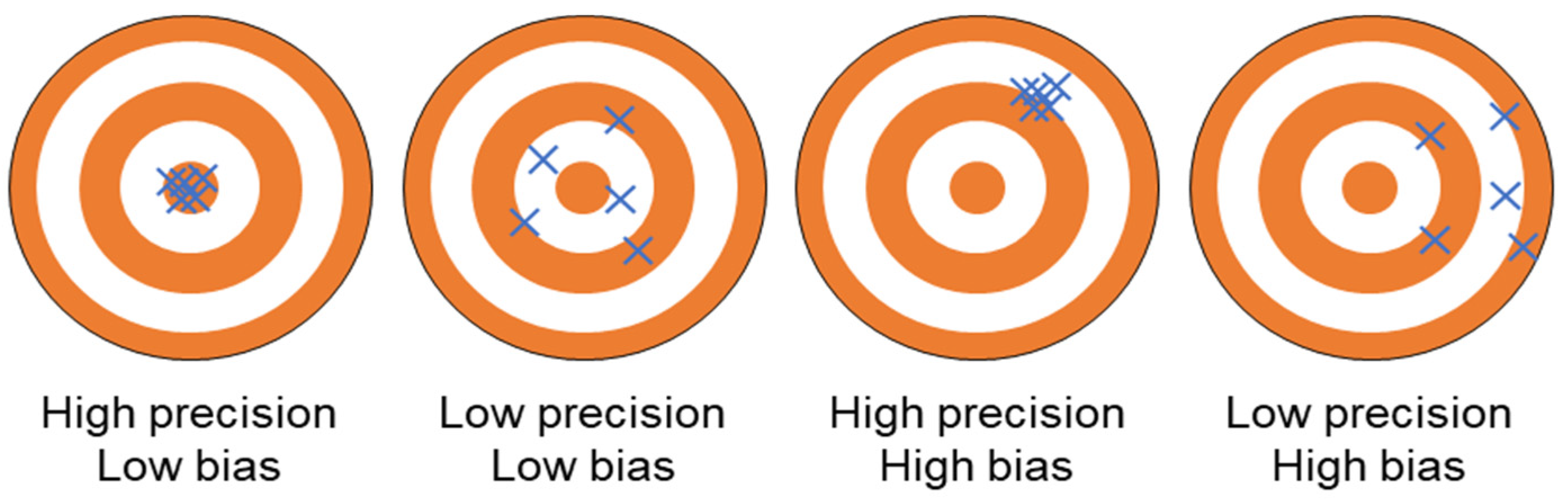
2.2. Sensor Errors
2.3. Control Logic for RTU and Single-Duct VAV System (ASHRAE Guideline 36)
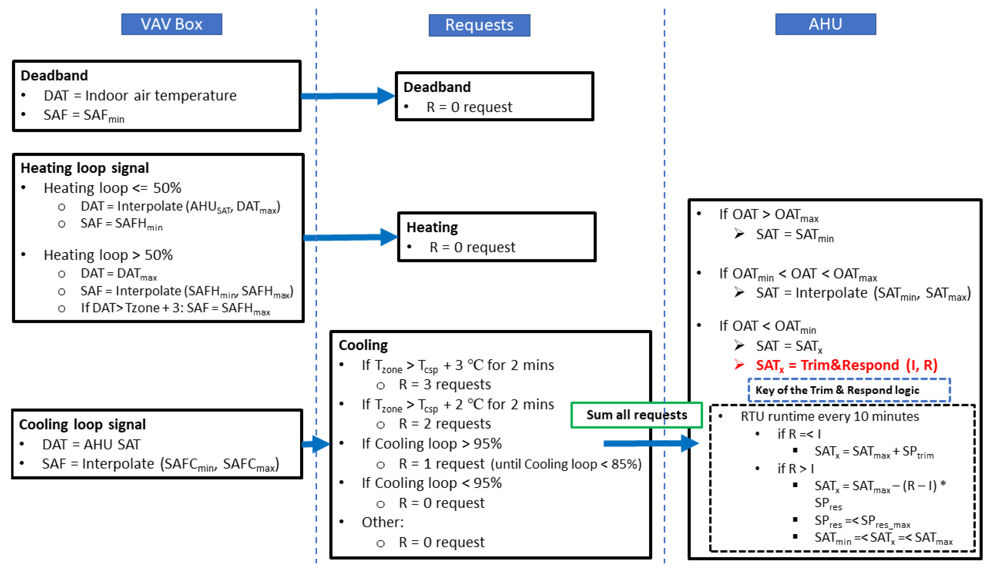
- AHU: Trim and Respond (T&R) Set Point Logic
- 2.
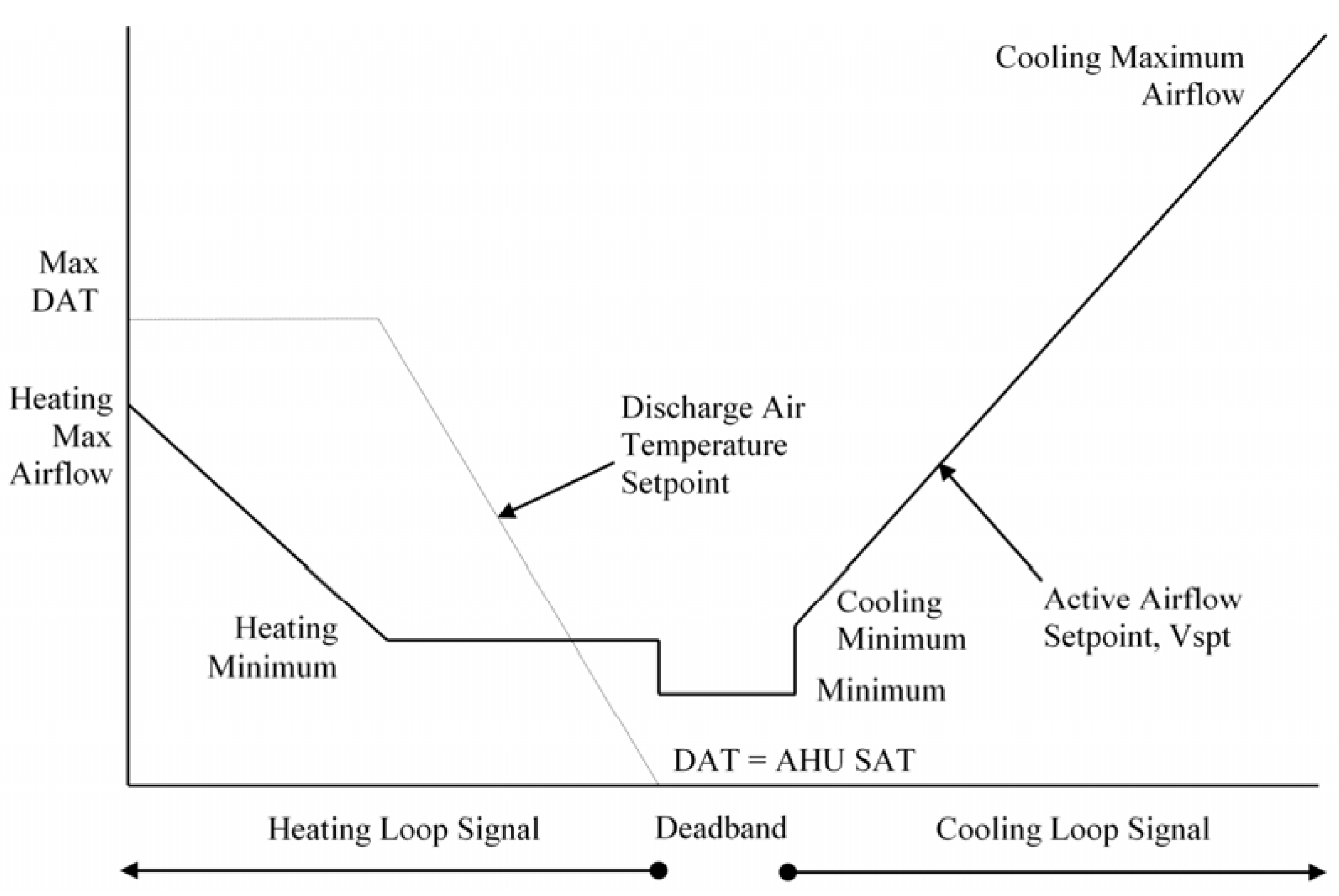
- VAV box control logic
- In the heating mode, when the heating loop is less than or equal to 50%, the discharge air (DA) set point temperature of the VAV box is increased from the RTU SAT to the maximum DA set point temperature of the VAV box, and the minimum SAF is maintained. When the heating loop is greater than 50%, if the DA temperature of the VAV box is greater than the IA temperature plus 3 °C, then the SAF of the VAV box is increased from the minimum SAF to the maximum SAF while maintaining the maximum DA set point temperature of the VAV box;
- In the cooling mode, the DA temperature of the VAV box is the same as the RTU SAT because no option exists to decrease the SAT using the VAV box. Therefore, VAV box control is linked with T&R control in the cooling season, when the VAV box control must be considered the RTU SAT. The four cooling SA set point temperature reset requests are as follows:
- If the IA temperature exceeds the indoor cooling set point temperature by 3 °C for 2 min and after the suppression period resulting from an RTU SA set point temperature change via the T&R control, then send three requests;
- Else, if the IA temperature exceeds the indoor cooling set point temperature by 2 °C for 2 min and after the suppression period resulting from an RTU SA set point temperature change via the T&R control, then send two requests;
- Else, if the cooling loop is greater than 95%, then send one request until the cooling loop is less than 85%;
- Else, if the cooling loop is less than 95%, then send no request.
- c.
- In the dead-band mode, when neither heating nor cooling are needed, the SAF is set to the minimum SAF, and the DA temperature of the VAV box is set to the RTU SAT.
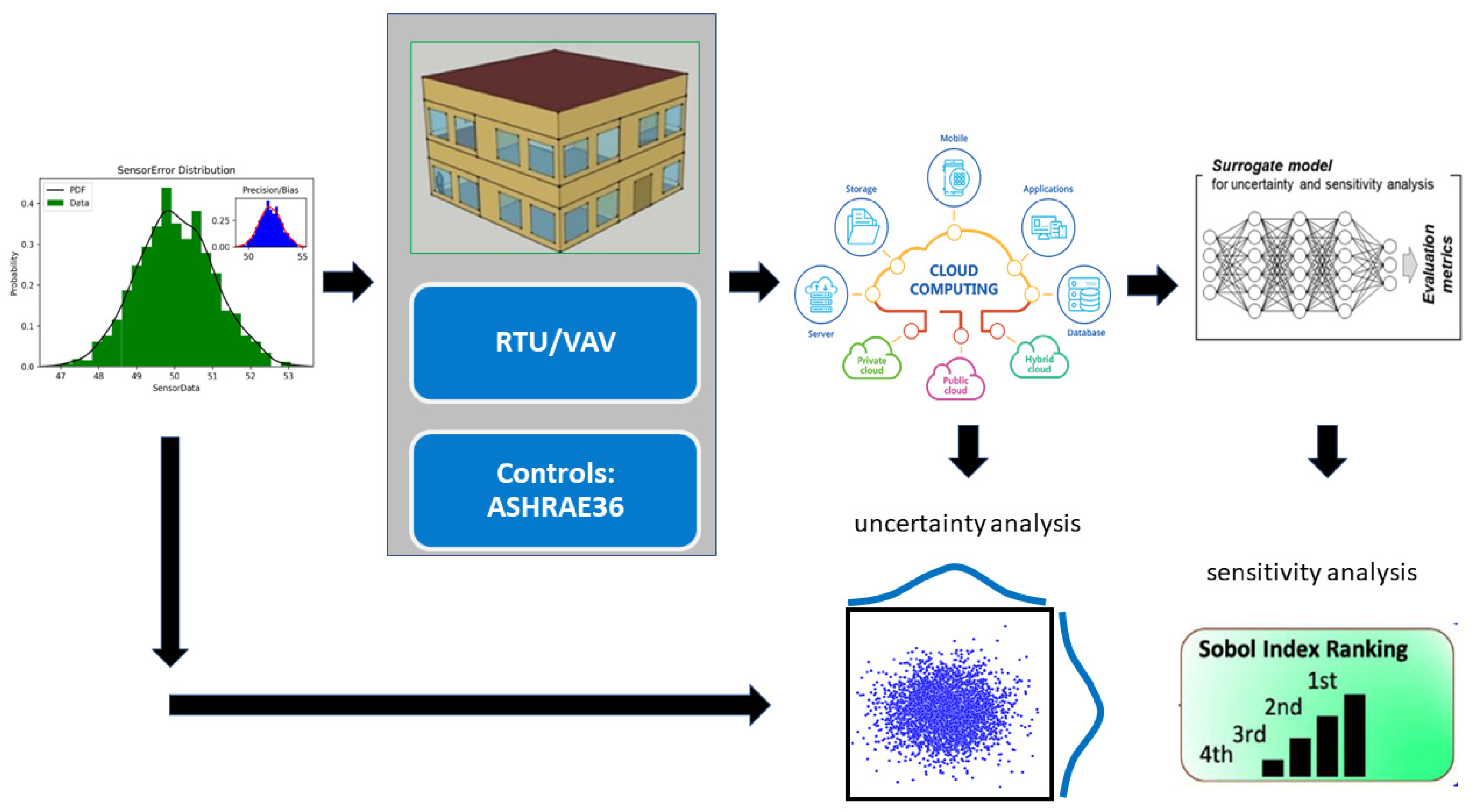
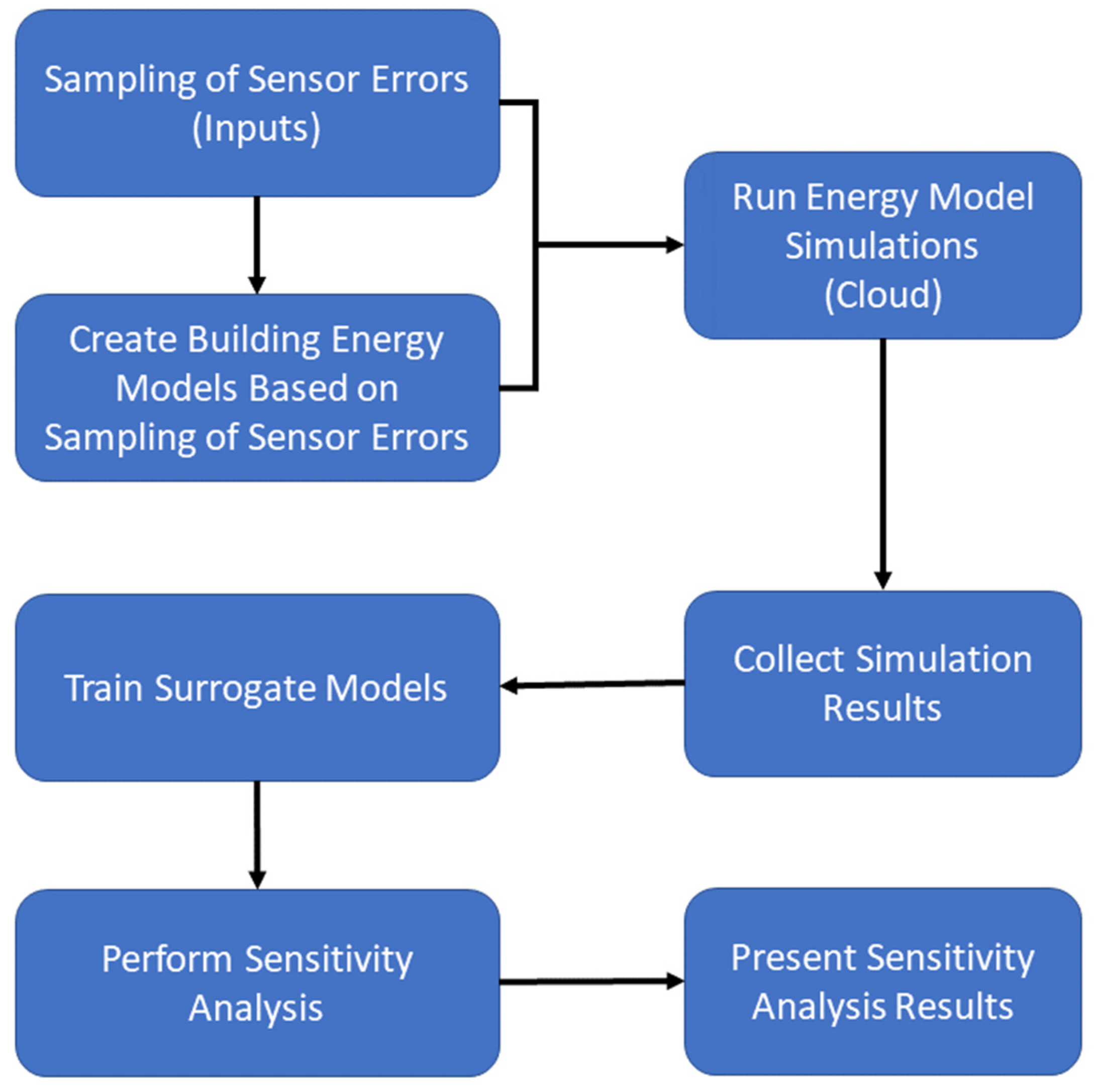
2.4. Large-Scale Simulation
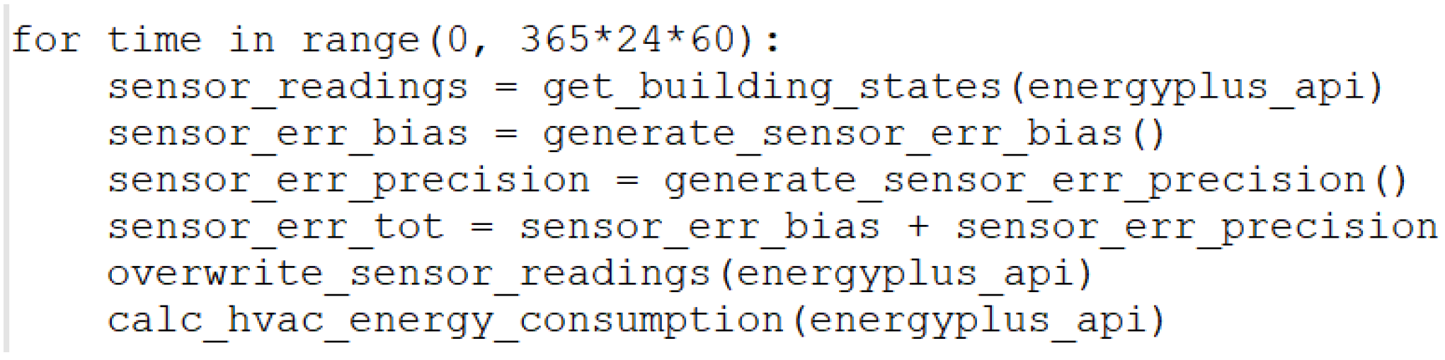
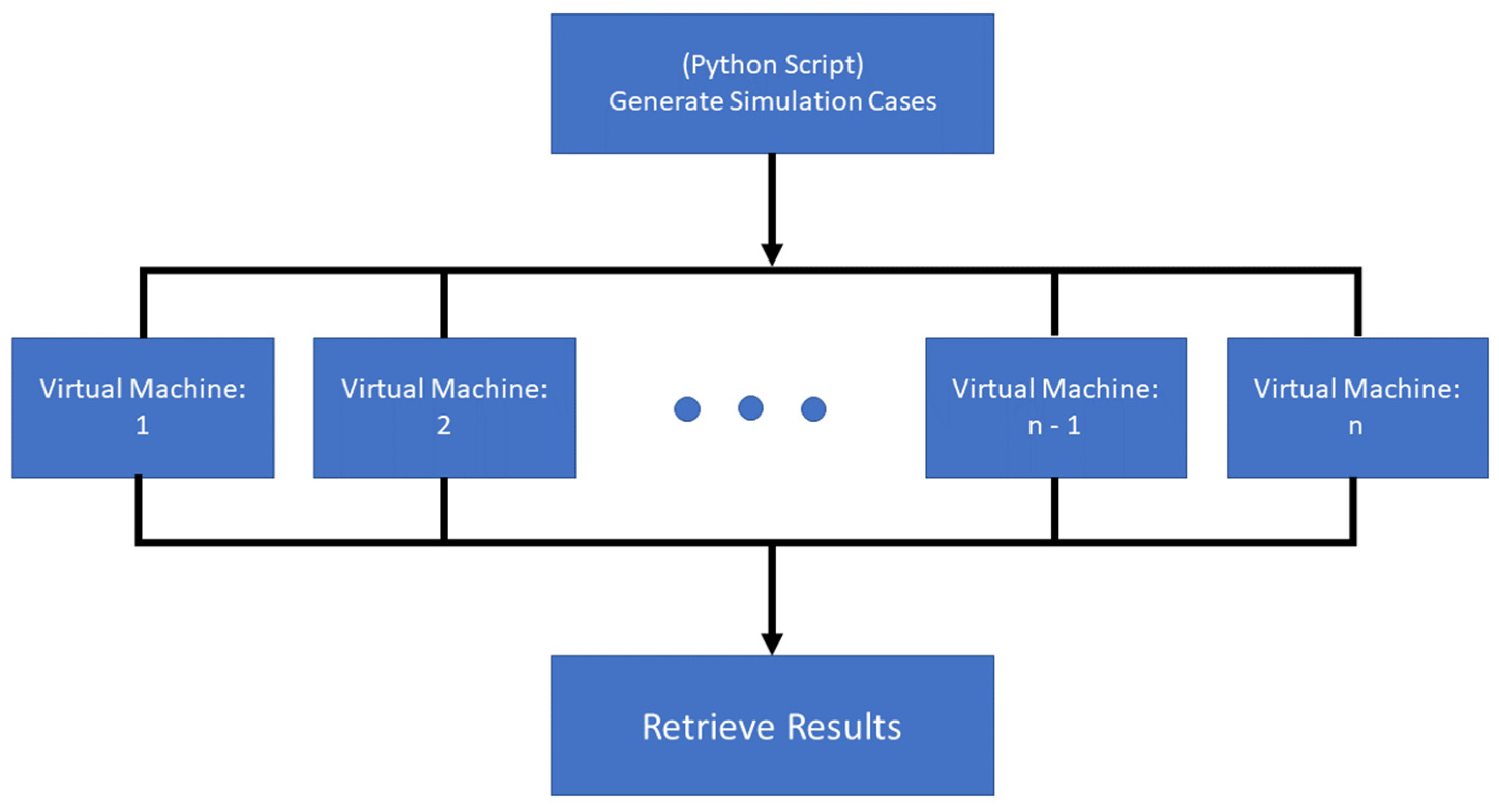
- (1)
- A Python script was developed to generate 3600 simulation input data files (IDF files). Each IDF file was associated with a Python class of sensor errors through Python EMS. During the simulation, at each time step, a new sensor error (including bias and precision) was injected into the ideal sensor readings from EnergyPlus;
- (2)
- After 3600 cases were generated, they were uploaded to the Azure cloud platform;
- (3)
- In the Azure cloud platform, a bash script selected the appropriate virtual machine configurations (e.g., memory and hard drive, as shown in Table 4) and a number of virtual machines. The team’s subscription included 300 nodes (virtual machines);
- (4)
- The Azure cloud provided a job scheduler, which automatically distributed all 3600 cases across 300 nodes;
- (5)
- The simulation ran automatically until all cases were accomplished;
- (6)
- Finally, all the results were selected to set up the data sets (inputs and outputs) to create the black-box models.
- (7)
- The configuration for the cloud is shown in Table 4.
2.5. Other Aspects
- (1)
- The baseline model was calibrated with the actual components and systems within the FRP2 building at ORNL campus. The input values for the HVAC system are from the measurement and nameplate values. The simulation results demonstrated the consistency between model and measurements [25];
- (2)
- The simulation cases have a total of 3600 sets. Each case matches with a sensor error module. In each timestep, the sensor error value will be injected into the model following the sensor error components (bias and precision). The energy consumption differences were easily calculated between baseline case and sensor-error case, which was caused by the sensor errors. If sensor errors were made to be zero all through the simulation timesteps, the same energy consumption was obtained with baseline model;
- (3)
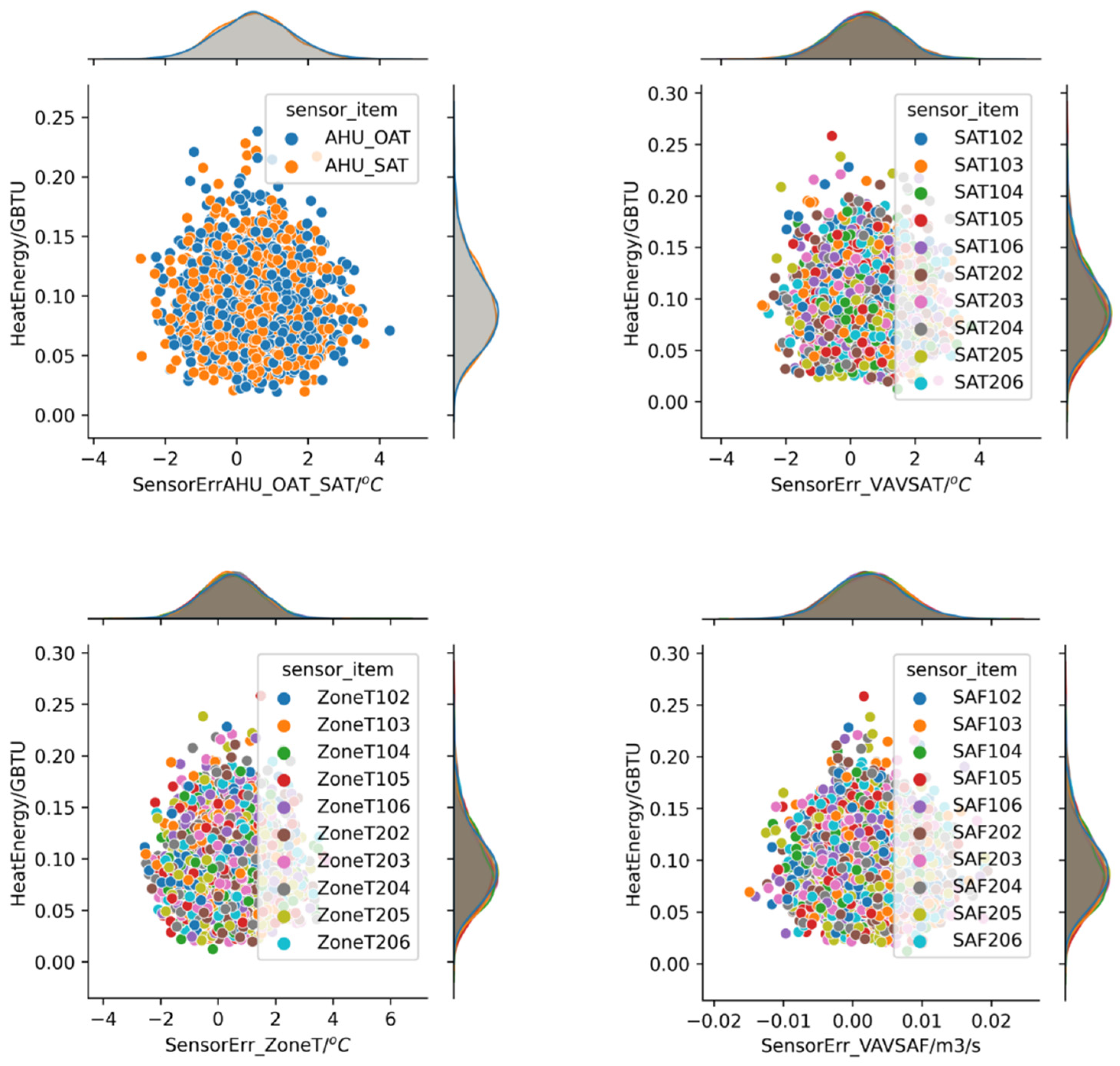
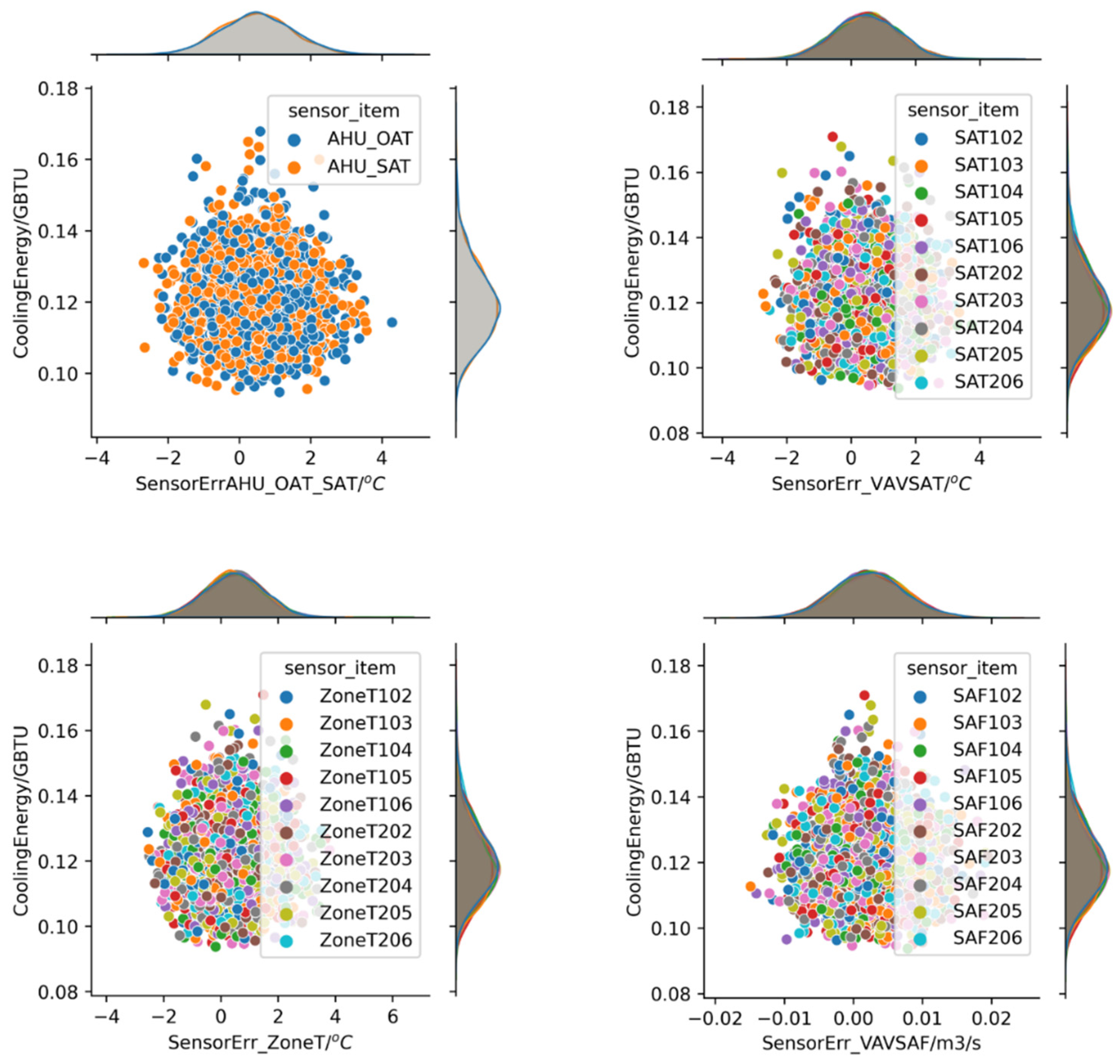
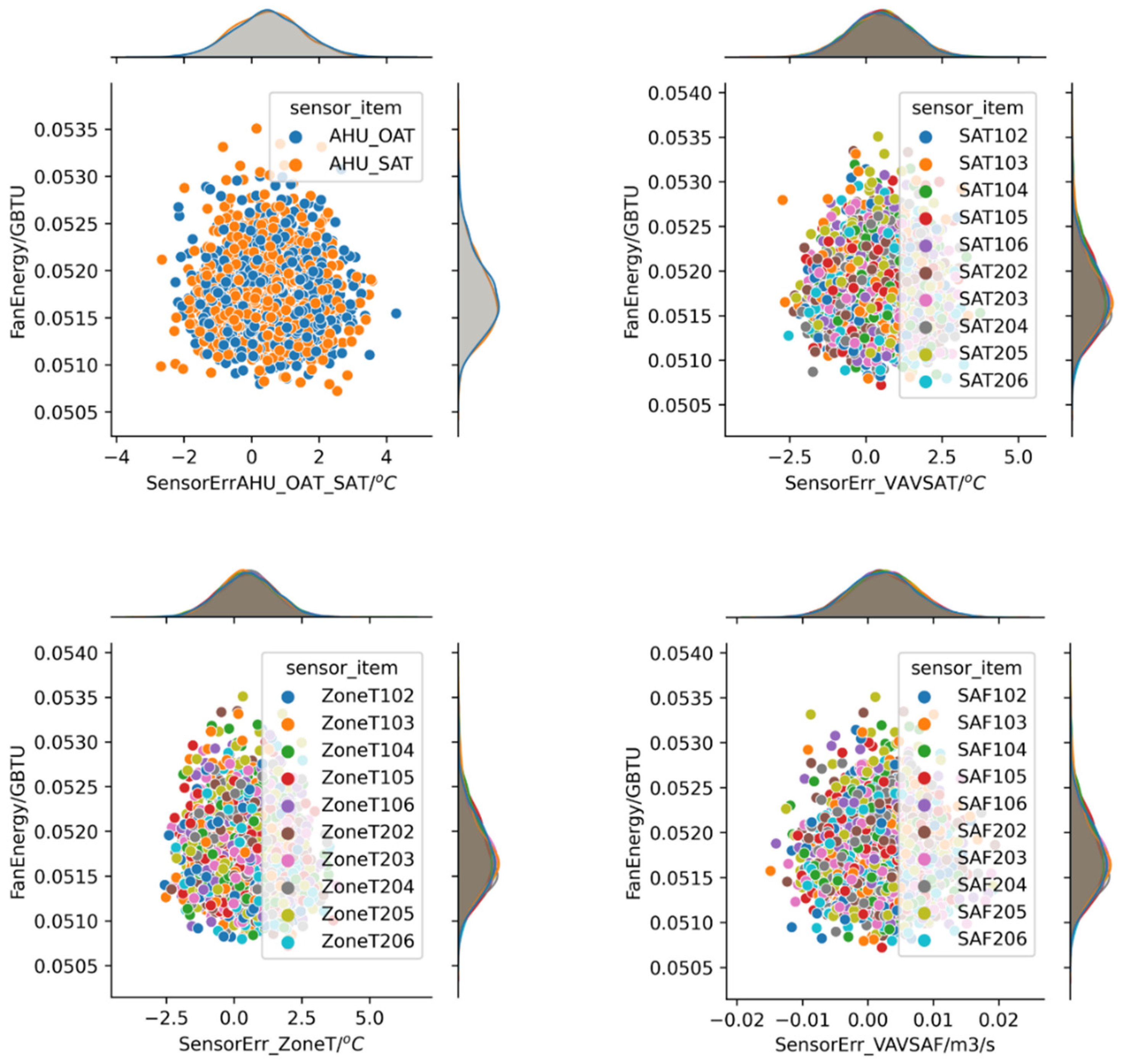
- We analyzed the results and see that they are reasonable for sensor errors. For example, (a) when we increase the sensor error to the zone temperature for cooling mode (lower zone temperature than it is supposed to be), we can see the energy consumption increasing. This is because the building model thinks it needs more cooling energy to meet the cooling setpoints. (b) When we increase the sensor error to the zone temperature sensor for heating mode (higher zone temperature than it is supposed to be), we can see the energy consumption decreasing. This is because the building model thinks it needs less heating energy to meet the heating setpoints;
- (4)
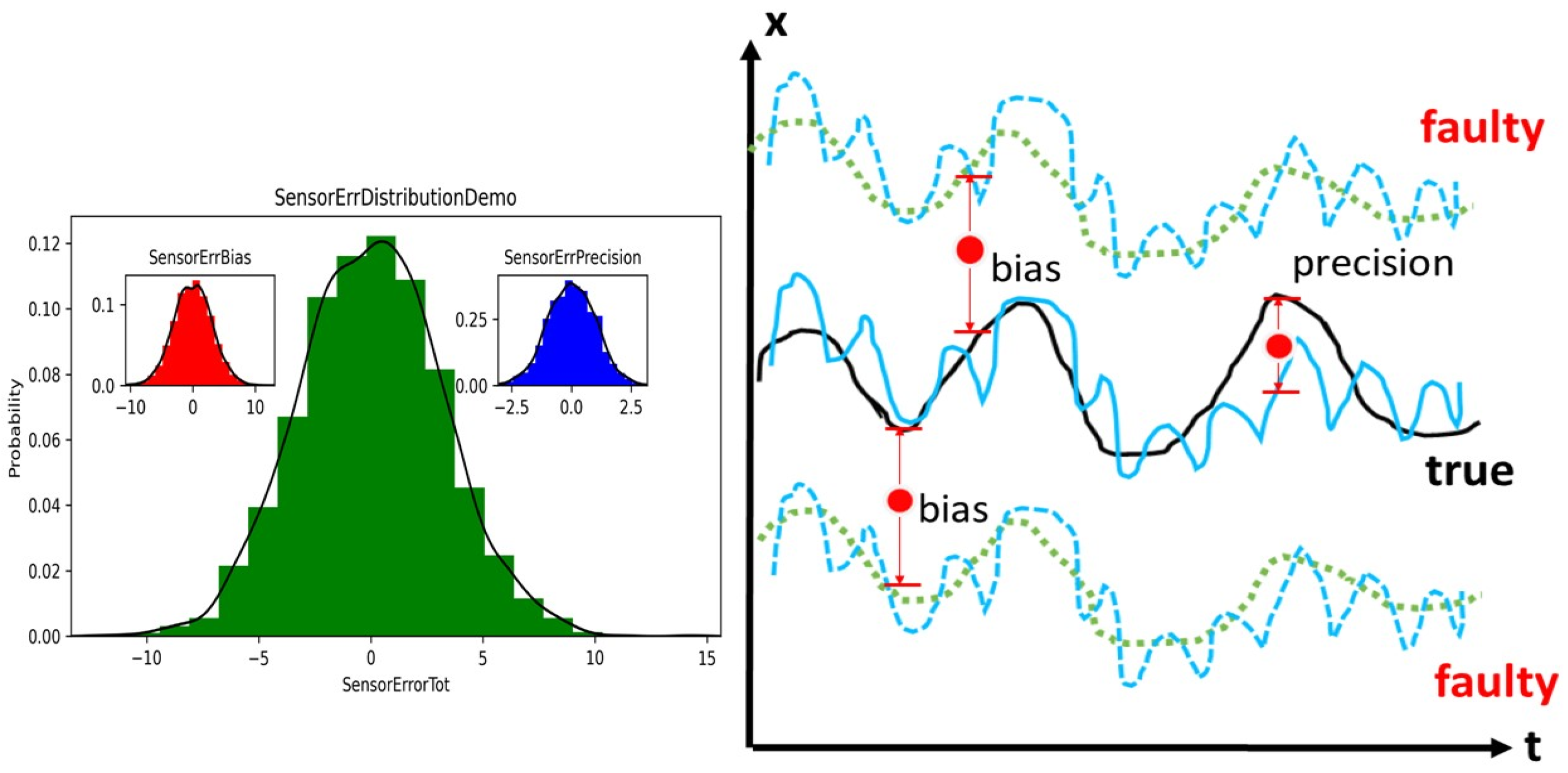
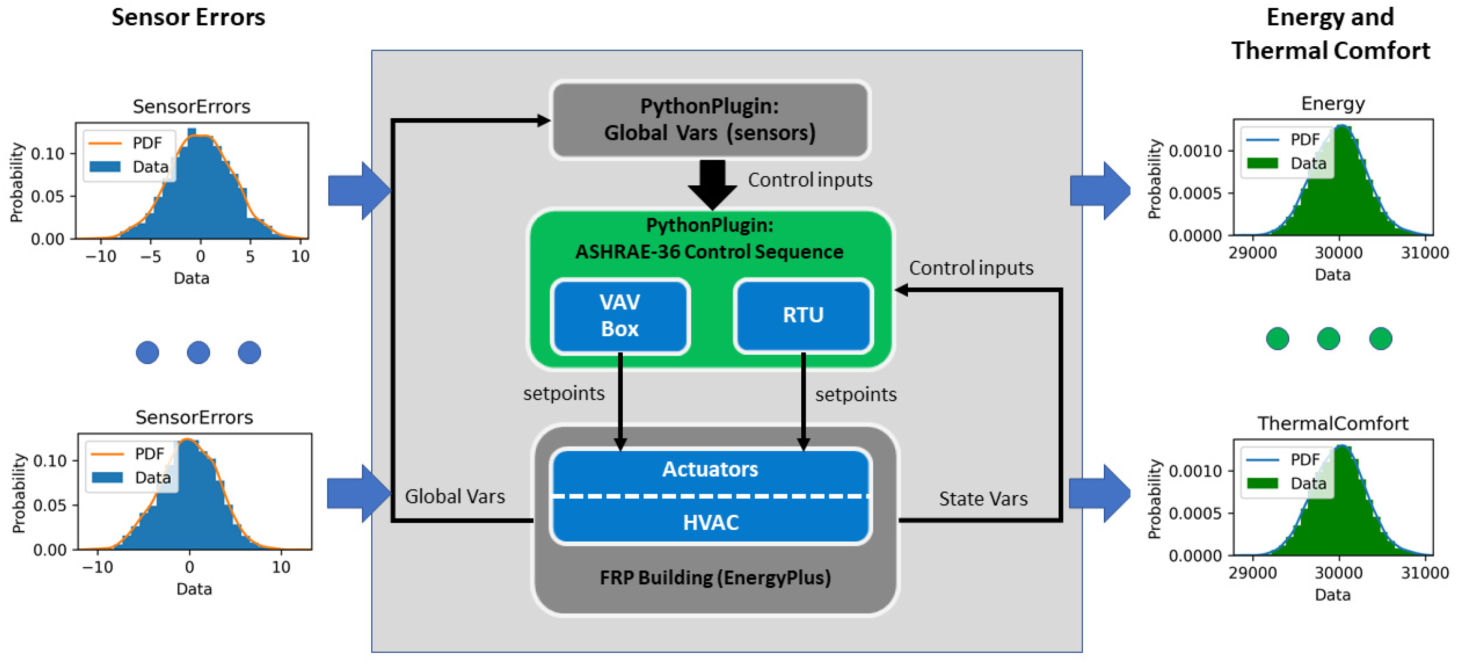
- To explain in detail, the sensor error in this study followed the normal distribution (Figure 4) and the sensor error range was calculated by bias sensor error plus precision error. For example, if the standard deviation of sensor error of the temperature sensor is 1 °C, the temperature sensor error range is within −3 °C and +3 °C with a probability of 99.76%. Similarly, the probability of sensor error range between −1 °C and +1 °C is about 68%. The probability of sensor error range within −2 °C and +2 °C is about 95.4%. The extreme cases are within 0.24% of scenarios on the two ends. Therefore, the differences (numbers) mentioned above occur when the sensor error is the largest (either positive or negative values).
3. Surrogate Model
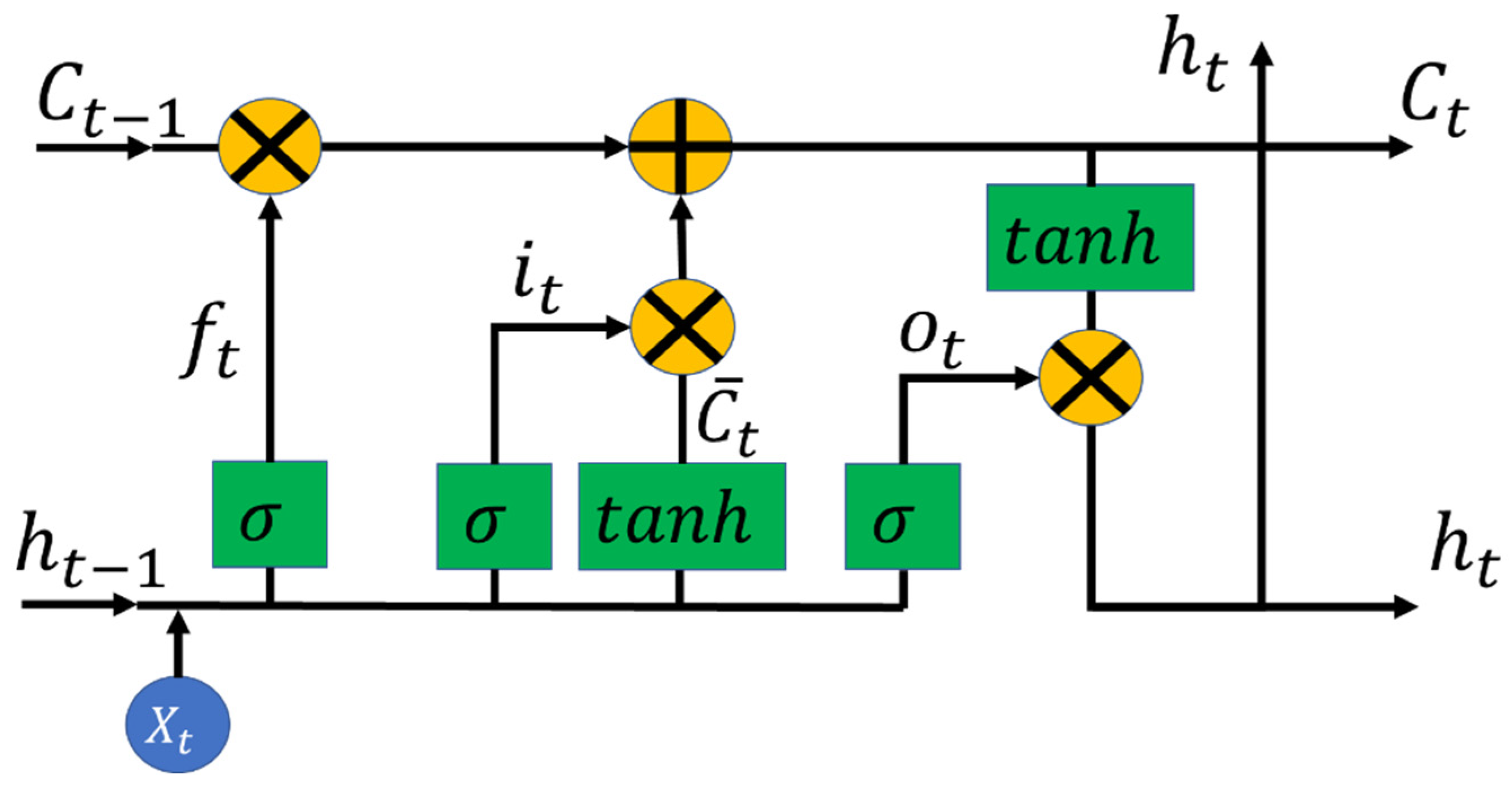
3.1. LSTM Setup
3.2. Training and Setting
3.3. Input/Output Variables
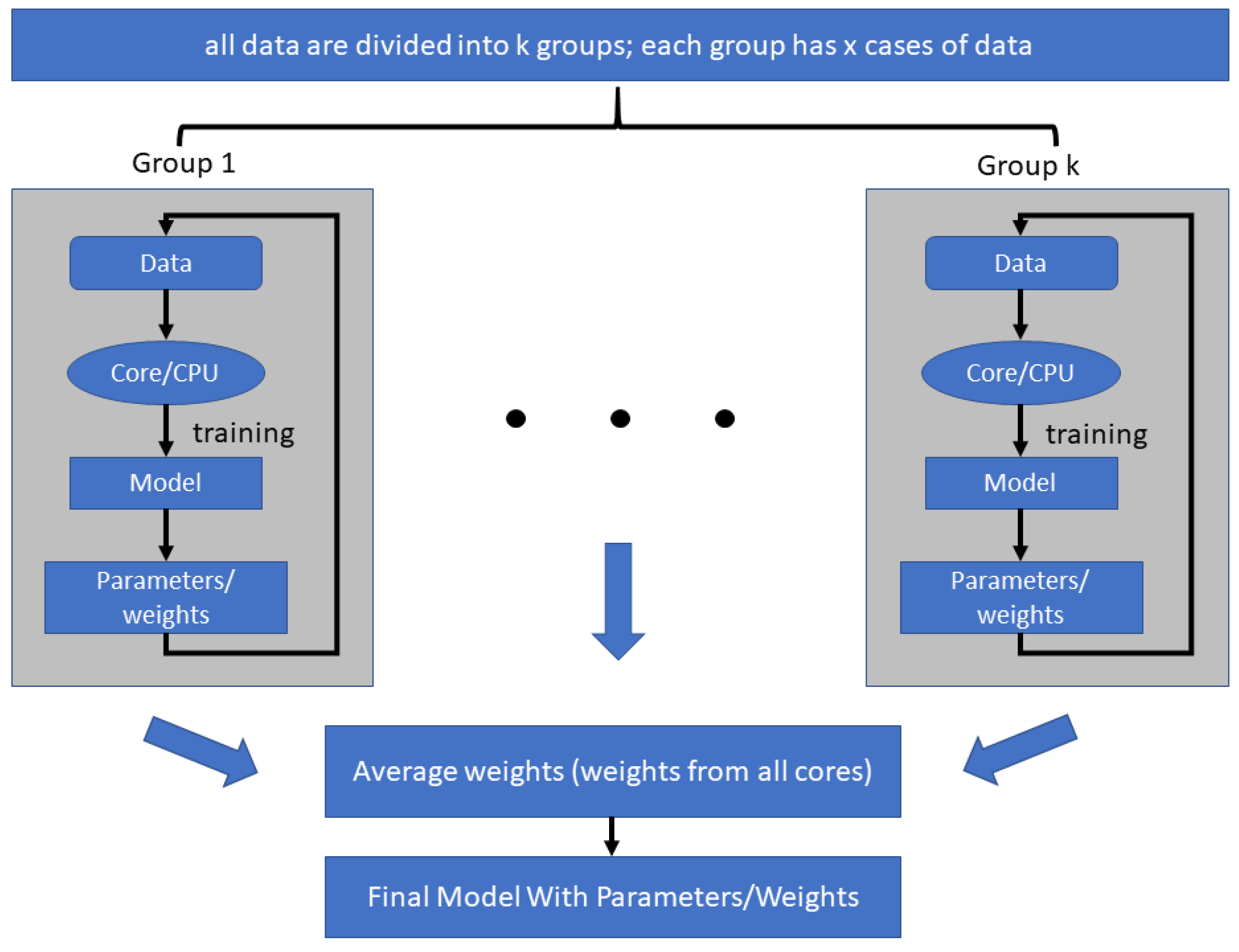
3.4. Workflow for Surrogate Model Training
4. Uncertainty Analysis
4.1. Uncertainty Analysis Setup
4.2. Uncertainty Analysis Results
5. Sensitivity Analysis
5.1. Sensitivity Analysis Principle
5.2. Sensitivity Analysis Results
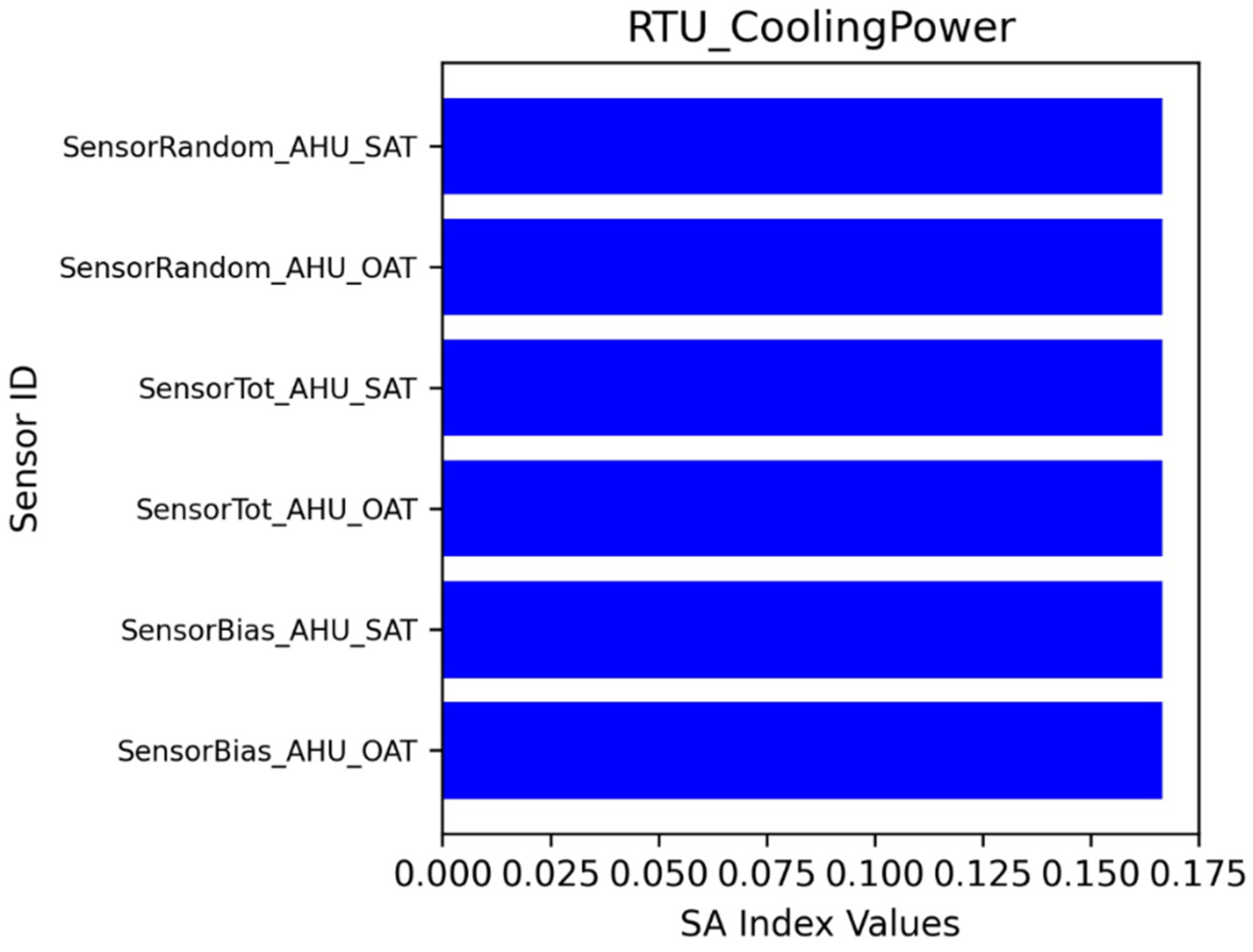
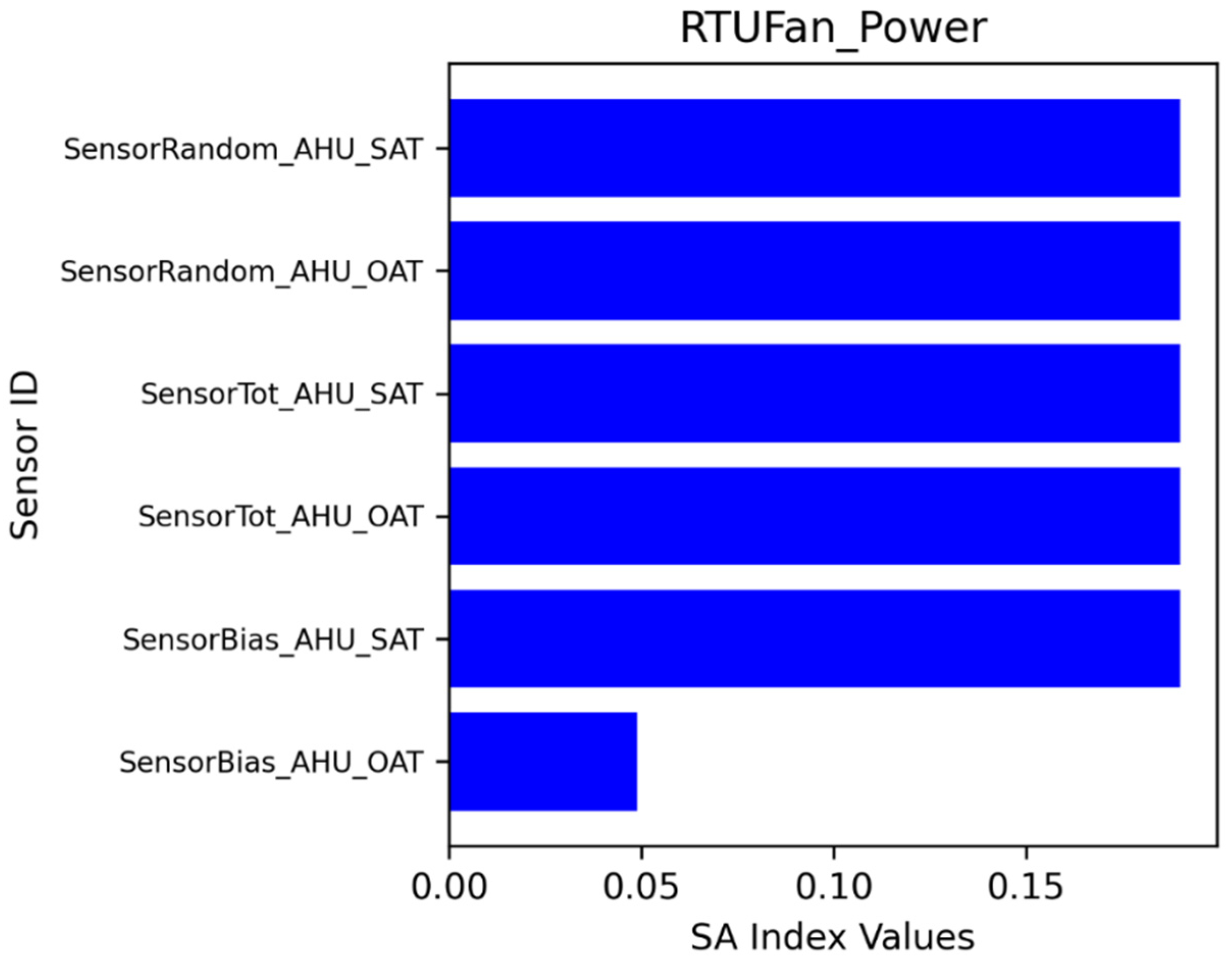
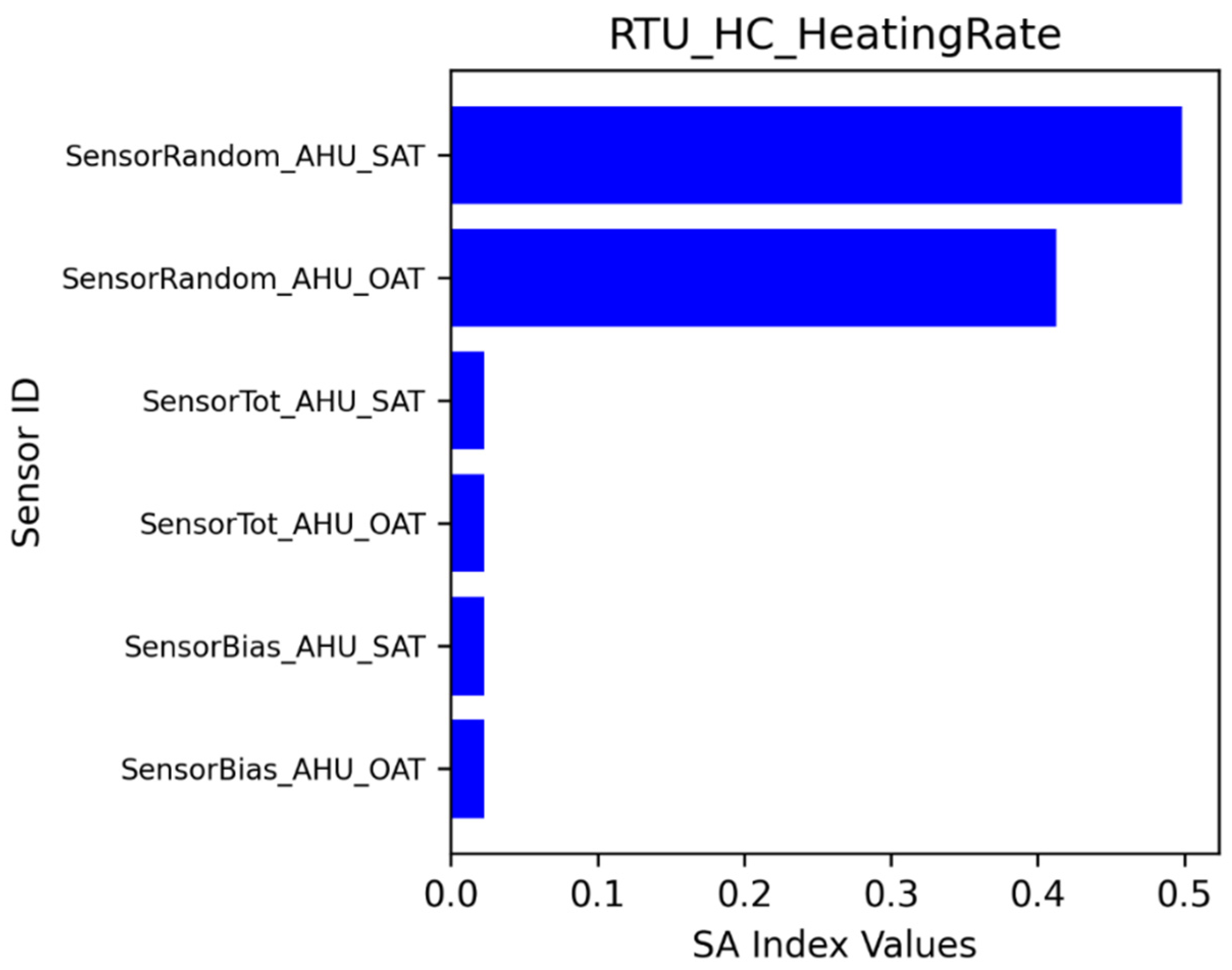
5.2.1. System SA Analysis
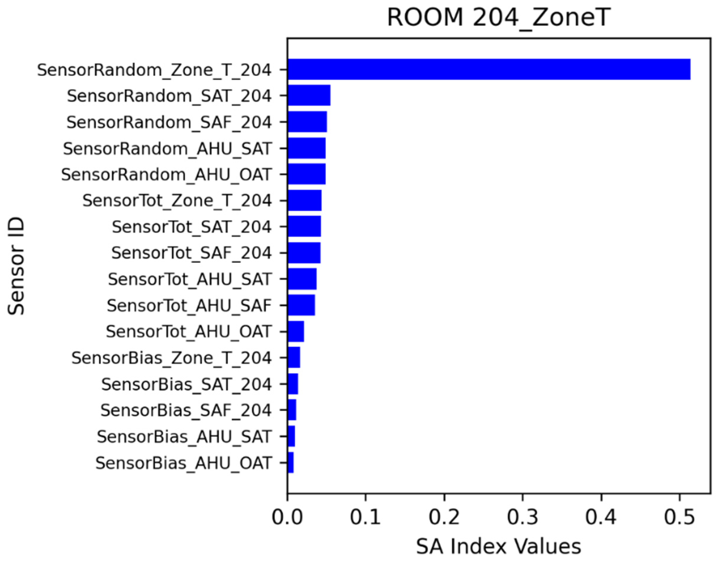
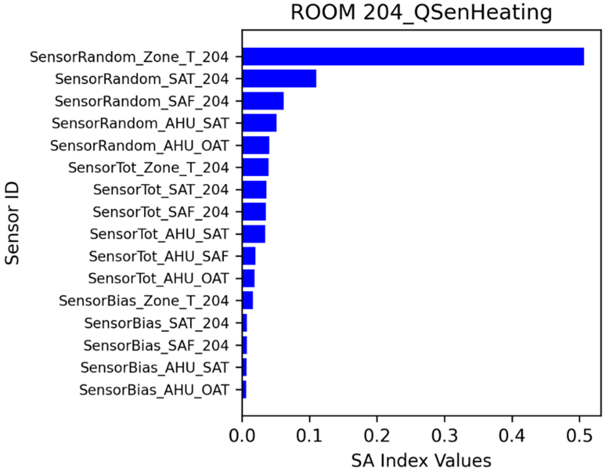
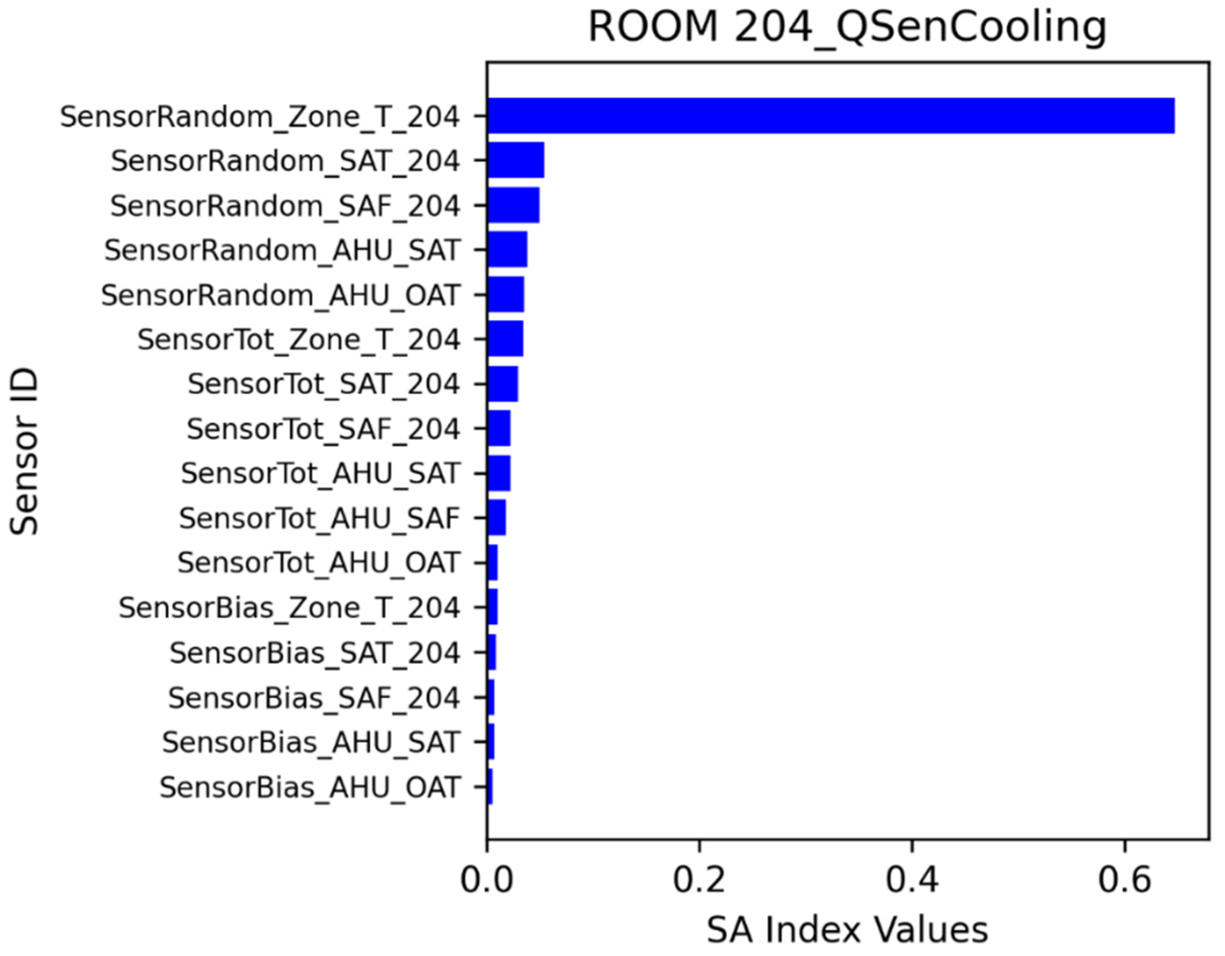
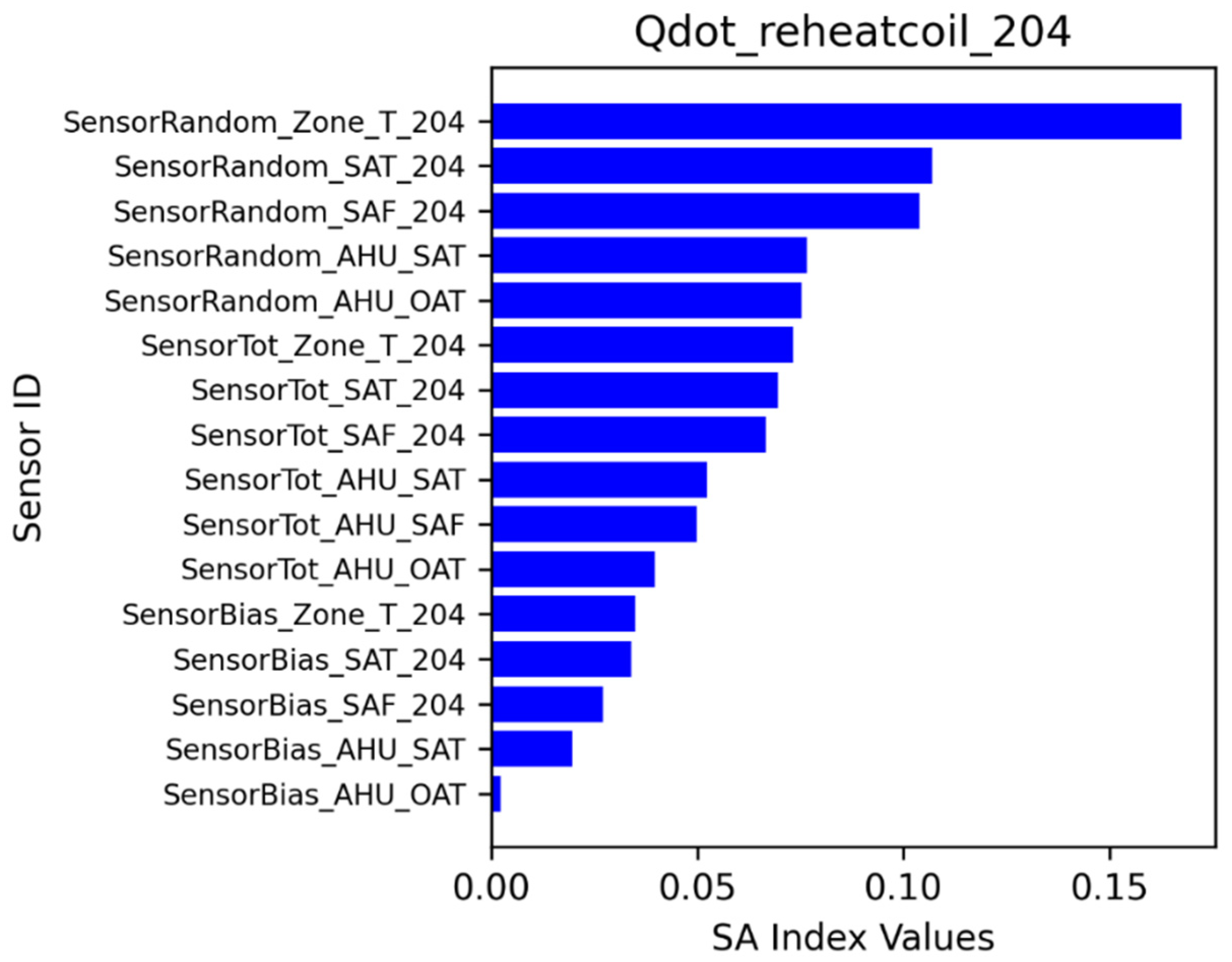
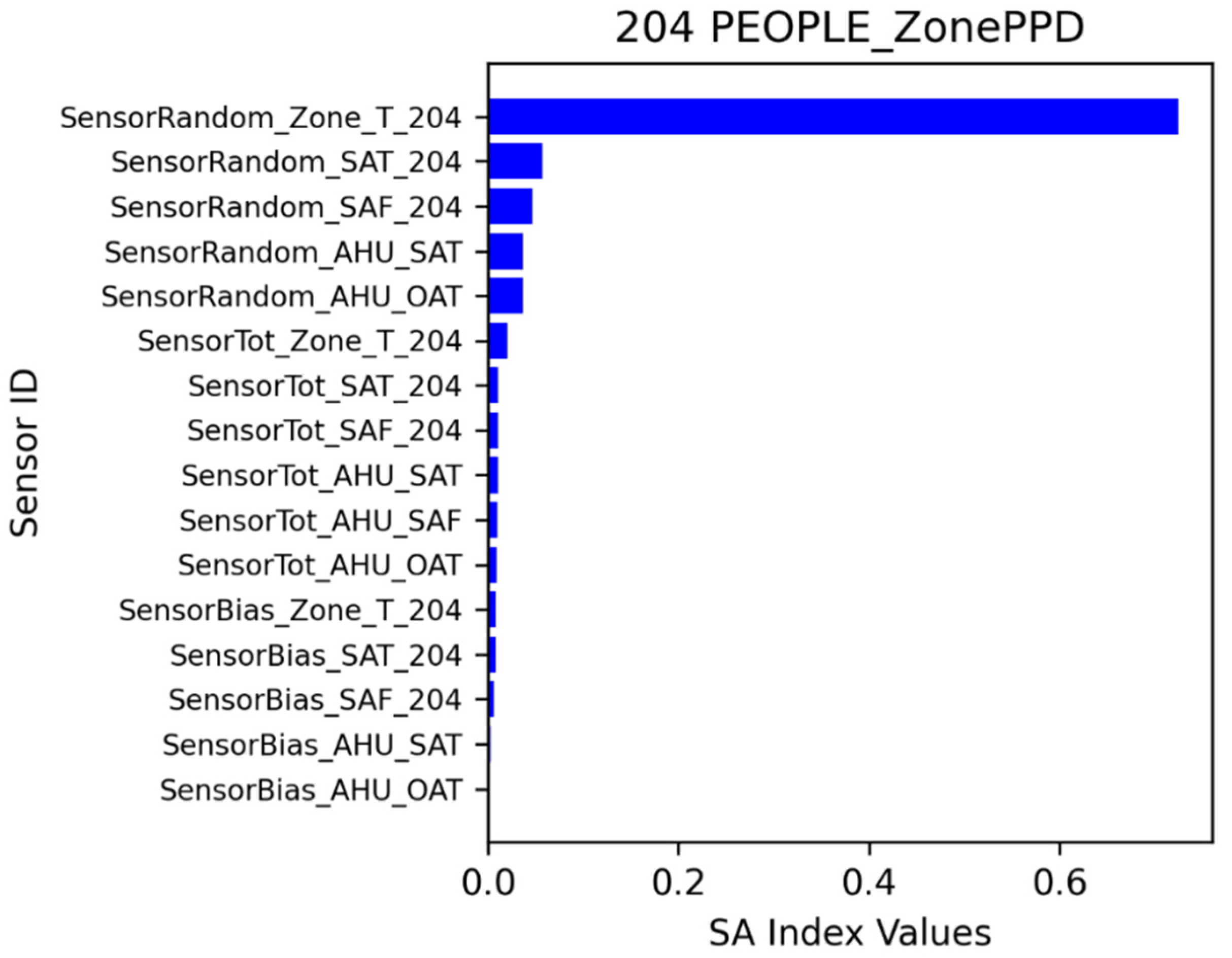
5.2.2. Zone 204 SA Analysis
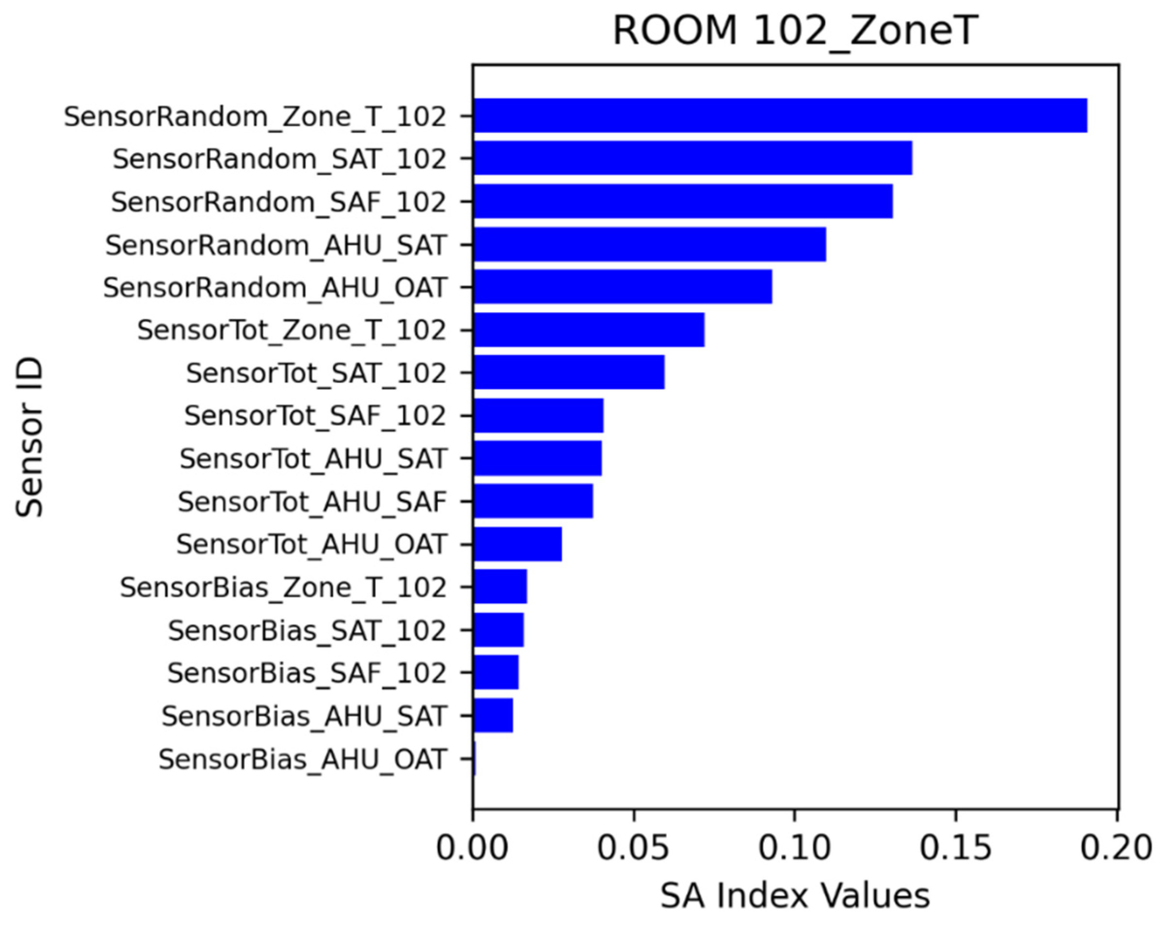
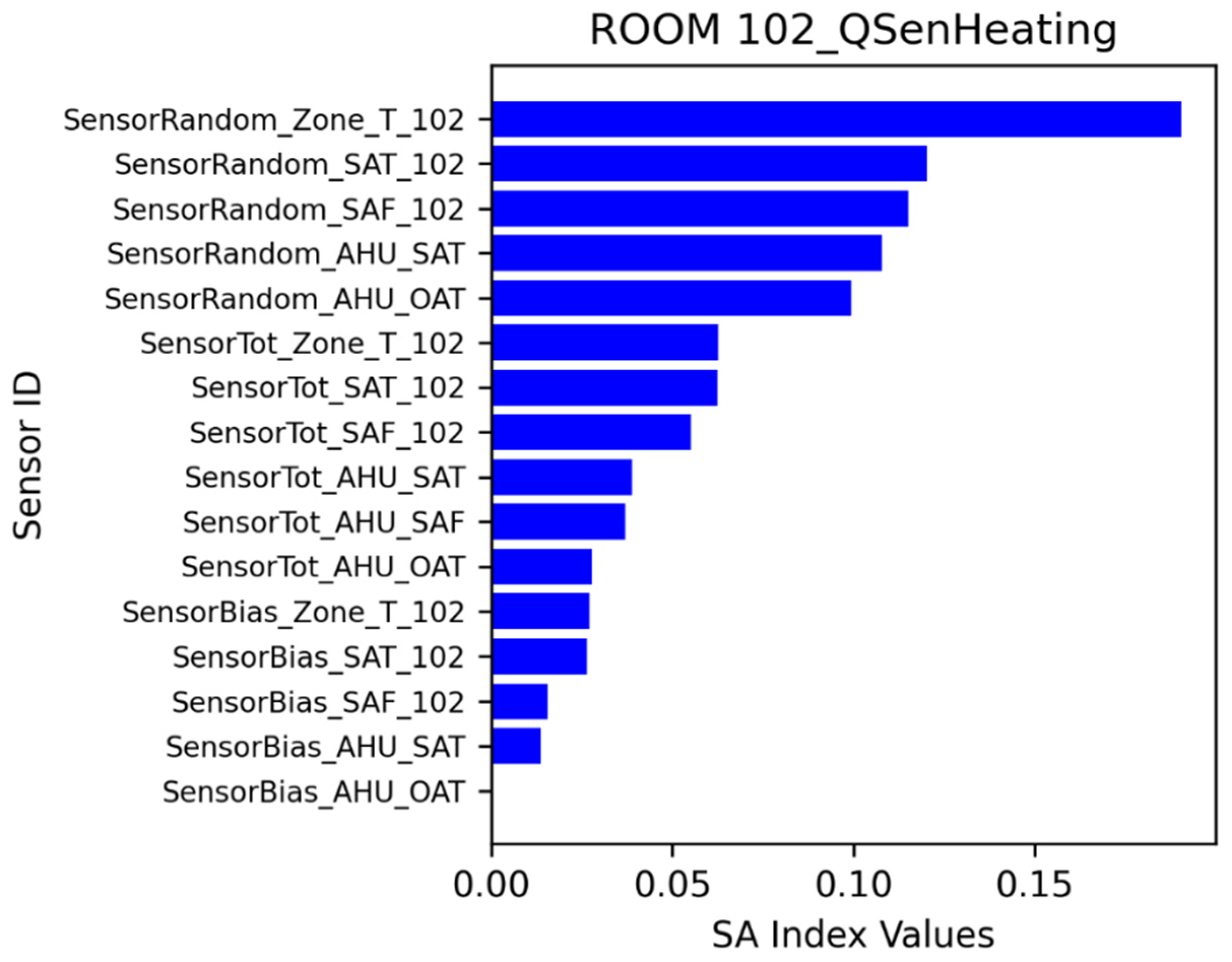
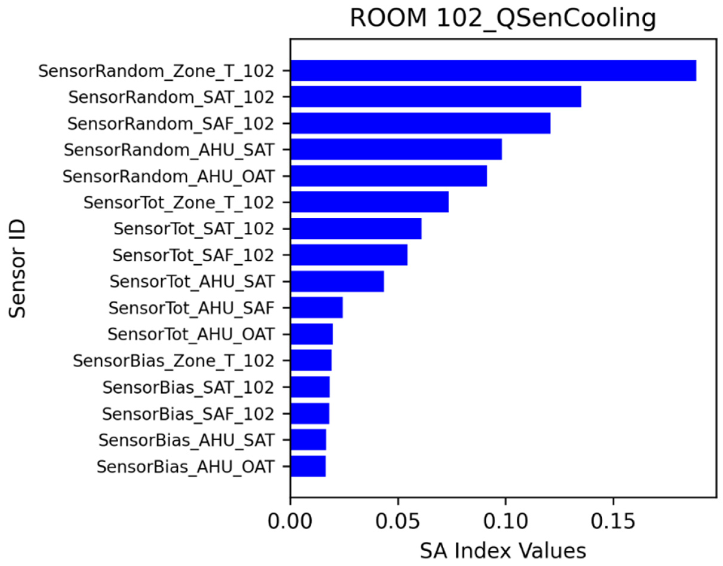
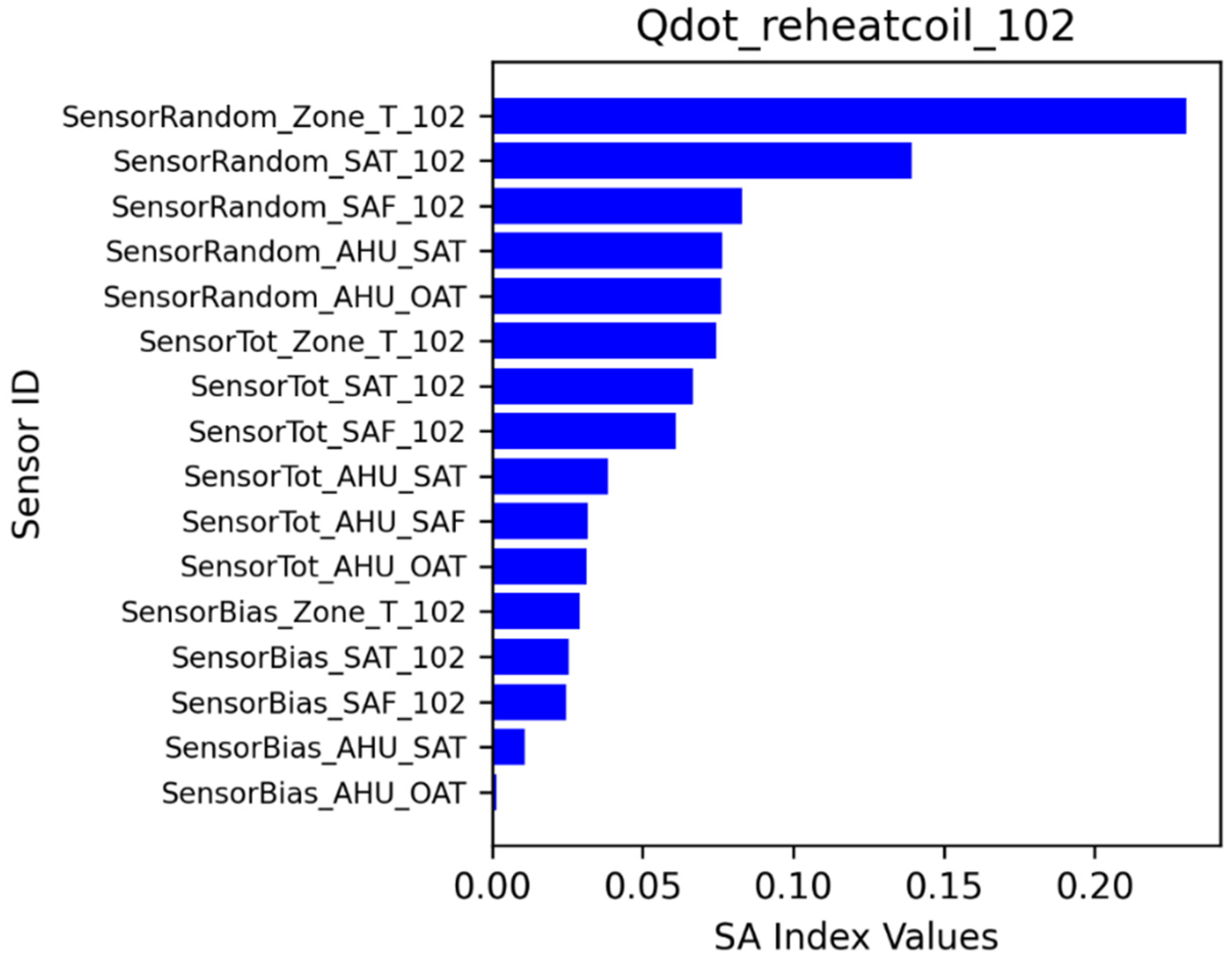
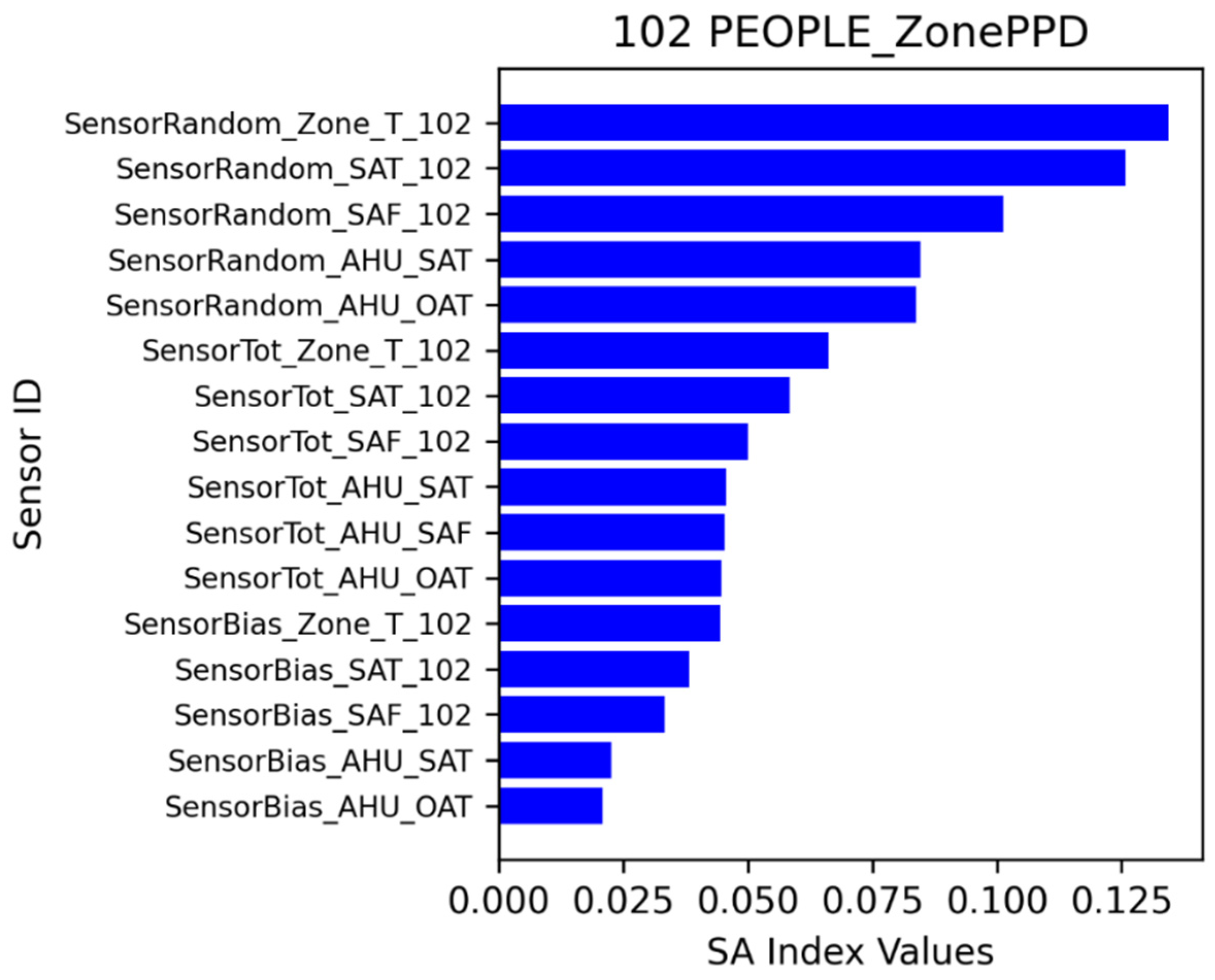
5.2.3. Zone 102 SA Analysis
6. Conclusions
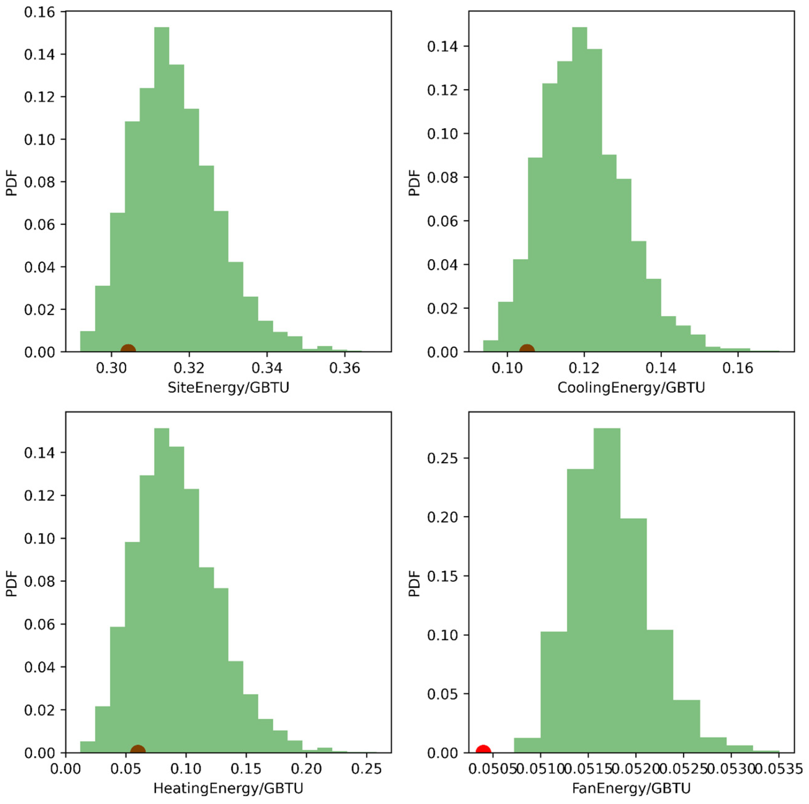
- The site energy differences could go −3.3% lower or 18.1% higher, compared with baseline;
- The heating energy differences could go −66.5% lower or 314.4% higher, compared with baseline;
- The cooling energy differences could go −11.5% lower or 65.0% higher, compared with baseline;
- The fan energy differences could go 0.15% lower or 6.9% higher, compared with baseline.
- Other sensitivity analysis methods will be used for comparative analysis;
- Other control strategies or HVAC systems will be used for more demonstrations.
Author Contributions
Funding
Acknowledgments
Conflicts of Interest
References
- Analysis & Projections—U.S. Energy Information Administration (EIA). Available online: https://www.eia.gov/analysis/index.php (accessed on 9 September 2022).
- Liu, X.; Lu, S.; Hughes, P.; Cai, Z. A comparative study of the status of GSHP applications in the United States and China. Renew. Sustain. Energy Rev. 2015, 48, 558–570. [Google Scholar] [CrossRef]
- Shen, B.; Ally, M.R. Energy and Exergy Analysis of Low-Global Warming Potential Refrigerants as Replacement for R410A in Two-Speed Heat Pumps for Cold Climates. Energies 2020, 13, 5666. [Google Scholar] [CrossRef]
- Bae, Y.; Bhattacharya, S.; Cui, B.; Lee, S.; Li, Y.; Zhang, L.; Im, P.; Adetola, V.; Vrabie, D.; Leach, M.; et al. Sensor impacts on building and HVAC controls: A critical review for building energy performance. Adv. Appl. Energy 2021, 4, 100068. [Google Scholar] [CrossRef]
- Li, Y.; O’Neill, Z. A critical review of fault modeling of HVAC systems in buildings. In Proceedings of the Building Simulation, Cambridge, UK, 11–12 September 2018; Springer: Berlin/Heidelberg, Germany, 2018; Volume 11, pp. 953–975. [Google Scholar]
- Basarkar, M.; Pang, X.; Wang, L.; Haves, P.; Hong, T. Modeling and Simulation of HVAC Faults in EnergyPlus; Lawrence Berkeley National Lab. (LBNL): Berkeley, CA, USA, 2011. [Google Scholar]
- Ni, K.; Ramanathan, N.; Chehade, M.N.H.; Balzano, L.; Nair, S.; Zahedi, S.; Kohler, E.; Pottie, G.; Hansen, M.; Srivastava, M. Sensor network data fault types. ACM Trans. Sens. Netw. (TOSN) 2009, 5, 1–29. [Google Scholar] [CrossRef]
- Lu, X.; O’Neill, Z.; Li, Y.; Niu, F. A novel simulation-based framework for sensor error impact analysis in smart building systems: A case study for a demand-controlled ventilation system. Appl. Energy 2020, 263, 114638. [Google Scholar] [CrossRef]
- Li, Y.; O’Neill, Z. An innovative fault impact analysis framework for enhancing building operations. Energy Build. 2019, 199, 311–331. [Google Scholar] [CrossRef]
- O’Neill, Z.D.; Li, Y.; Cheng, H.C.; Zhou, X.; Taylor, S.T. Energy savings and ventilation performance from CO2-based demand controlled ventilation: Simulation results from ASHRAE RP-1747 (ASHRAE RP-1747). Sci. Technol. Built Environ. 2020, 26, 257–281. [Google Scholar] [CrossRef]
- Ye, Y.; Chen, Y.; Zhang, J.; Pang, Z.; O’Neill, Z.; Dong, B.; Cheng, H. Energy-saving potential evaluation for primary schools with occupant-centric controls. Appl. Energy 2021, 293, 116854. [Google Scholar] [CrossRef]
- Pang, Z.; Chen, Y.; Zhang, J.; O’Neill, Z.; Cheng, H.; Dong, B. Nationwide HVAC energy-saving potential quantification for office buildings with occupant-centric controls in various climates. Appl. Energy 2020, 279, 115727. [Google Scholar] [CrossRef]
- Maasoumy, M.; Razmara, M.; Shahbakhti, M.; Vincentelli, A. Handling model uncertainty in model predictive control for energy efficient buildings. Energy Build. 2014, 77, 377–392. [Google Scholar] [CrossRef]
- Bengea, S.; Adetola, V.; Kang, K.; Liba, M.J.; Vrabie, D.; Bitmead, R.; Narayanan, S. Parameter estimation of a building system model and impact of estimation error on closed-loop performance. In Proceedings of the 2011 50th IEEE Conference on Decision and Control and European Control Conference, Orlando, FL, USA, 12–15 December 2011; pp. 5137–5143. [Google Scholar]
- Chen, J.; Zhang, L.; Li, Y.; Shi, Y.; Gao, X.; Hu, Y. A review of computing-based automated fault detection and diagnosis of heating, ventilation and air conditioning systems. Renew. Sustain. Energy Rev. 2022, 161, 112395. [Google Scholar] [CrossRef]
- Yoon, S.; Yu, Y.; Wang, J.; Wang, P. Impacts of HVACR temperature sensor offsets on building energy performance and occupant thermal comfort. In Proceedings of the Building Simulation, Rome, Italy, 2–4 September 2019; Springer: Berlin/Heidelberg, Germany, 2019; Volume 12, pp. 259–271. [Google Scholar]
- Kim, J.; Frank, S.; Braun, J.E.; Goldwasser, D. Representing small commercial building faults in energyplus, Part I: Model development. Buildings 2019, 9, 233. [Google Scholar] [CrossRef]
- Kim, J.; Frank, S.; Im, P.; Braun, J.E.; Goldwasser, D.; Leach, M. Representing small commercial building faults in EnergyPlus, part II: Model validation. Buildings 2019, 9, 239. [Google Scholar] [CrossRef]
- Zhao, Y.; Li, T.; Zhang, X.; Zhang, C. Artificial intelligence-based fault detection and diagnosis methods for building energy systems: Advantages, challenges and the future. Renew. Sustain. Energy Rev. 2019, 109, 85–101. [Google Scholar] [CrossRef]
- Wang, P.; Li, J.; Yoon, S.; Zhao, T.; Yu, Y. The detection and correction of various faulty sensors in a photovoltaic thermal heat pump system. Appl. Therm. Eng. 2020, 175, 115347. [Google Scholar] [CrossRef]
- Gunes, V.; Peter, S.; Givargis, T. Improving energy efficiency and thermal comfort of smart buildings with HVAC systems in the presence of sensor faults. In Proceedings of the 2015 IEEE 17th International Conference on High Performance Computing and Communications, New York, NY, USA, 24–26 August 2015; IEEE: Piscataway, NJ, USA, 2015; pp. 945–950. [Google Scholar]
- Zhang, L.; Leach, M.; Bae, Y.; Cui, B.; Bhattacharya, S.; Lee, S.; Im, P.; Adetola, V.; Vrabie, D.; Kuruganti, T. Sensor impact evaluation and verification for fault detection and diagnostics in building energy systems: A review. Adv. Appl. Energy 2021, 3, 100055. [Google Scholar] [CrossRef]
- Cheung, H.; Braun, J.E. Empirical modeling of the impacts of faults on water-cooled chiller power consumption for use in building simulation programs. Appl. Therm. Eng. 2016, 99, 756–764. [Google Scholar] [CrossRef]
- ASHRAE Guideline 36-2018: High-Performance Sequences of Operation for HVAC Systems 2022. Available online: https://www.techstreet.com/ashrae/standards/guideline-36-2018-high-performance-sequences-of-operation-for-hvac-systems (accessed on 9 September 2022).
- Im, P.; Joe, J.; Bae, Y.; New, J.R. Empirical validation of building energy modeling for multi-zones commercial buildings in cooling season. Appl. Energy 2020, 261, 114374. [Google Scholar] [CrossRef]
- Taylor, S. Resetting setpoints using trim & respond logic. Ashrae J. 2015, 11, 52–57. [Google Scholar]
- Hochreiter, S.; Schmidhuber, J. Long short-term memory. Neural Comput. 1997, 9, 1735–1780. [Google Scholar] [CrossRef]
- Tian, W. A review of sensitivity analysis methods in building energy analysis. Renew. Sustain. Energy Rev. 2013, 20, 411–419. [Google Scholar] [CrossRef]
- Pang, Z.; O’Neill, Z.; Li, Y.; Niu, F. The role of sensitivity analysis in the building performance analysis: A critical review. Energy Build. 2020, 209, 109659. [Google Scholar] [CrossRef]


| Location | Measurement | Priority | Location | Measurement | Priority |
|---|---|---|---|---|---|
| Room | IA temperature | 1 | RTU | OA CO2 | 4 |
| Room | IA humidity | 3 | RTU | OA flow rate | 3 |
| Room | IA CO2 | 4 | RTU | SA temperature | 1 |
| Room | Lighting condition | 5 | RTU | SA humidity | 3 |
| Room | Occupancy | 5 | RTU | SA CO2 | 4 |
| VAV box | SA temperature | 1 | RTU | SA flow rate | 3 |
| VAV box | SA humidity | 3 | RTU | RA temperature | 2 |
| VAV box | SA flow rate | 1 | RTU | RA humidity | 3 |
| Main duct | Static pressure | 2 | RTU | RA CO2 | 4 |
| Exhaust fan | EA temperature | 4 | RTU | RA flow rate | 3 |
| Exhaust fan | EA humidity | 4 | RTU | MA temperature | 2 |
| Exhaust fan | EA flow rate | 4 | RTU | MA humidity | 3 |
| Exhaust fan | EA CO2 | 4 | RTU | MA CO2 | 4 |
| Other | Plug load | 5 | RTU | MA flow rate | 3 |
| Other | Lighting load | 5 | RTU | Refrigerant temperature | 5 |
| RTU | OA temperature | 1 | RTU | Refrigerant pressure | 5 |
| RTU | OA humidity | 3 | RTU | Refrigerant flow rate | 5 |
| Location | Measurement | Priority | Note |
|---|---|---|---|
| Room | IA temperature | 1 | IA temperature |
| VAV box | SAT | 1 | VAV box SAT |
| VAV box | SAF | 1 | VAV box SAF |
| RTU | OAT | 1 | OAT |
| RTU | SAT | 1 | SAT |
| Measured Data | Range |
|---|---|
| Outdoor air temperature | −50~100 °C |
| Indoor air temperature | |
| Supply air temperature | |
| Supply airflow rate | 0~15.24 m/s |
| Location | Measurement | Bias | Precision |
|---|---|---|---|
| Room | IA temperature (°C) | 1 | 0.1 |
| VAV box | SAT (°C) | 1 | 0.1 |
| VAV box | SAF (m3/s) | 0.005 | 0.0005 |
| RTU | OAT (°C) | 1 | 0.1 |
| RTU | SAT (°C) | 1 | 0.1 |
| Variable Name | Quantity |
|---|---|
| OAT | 1 |
| OA relative humidity | 1 |
| OA pressure | 1 |
| Wind speed | 1 |
| Wind direction | 1 |
| Horizontal infrared radiation rate | 1 |
| Diffuse solar radiation rate | 1 |
| Direct solar radiation rate | 1 |
| Lighting energy | 1 |
| Internal heat gains: equipment | 1 |
| People activity | 1 |
| SensorBias: AHU OAT | 1 |
| SensorPrecision: AHU OAT | 1 |
| SensorTotalError: AHU OAT | 1 |
| SensorBias: AHU SAT | 1 |
| SensorPrecision: AHU SAT | 1 |
| SensorTotalError: AHU SAT | 1 |
| SensorBias: zone VAV SAF | 10 |
| SensorPrecision: zone VAV SAF | 10 |
| SensorTotalError: zone VAV SAF | 10 |
| SensorBias: zone VAV SAT | 10 |
| SensorPrecision: zone VAV SAT | 10 |
| SensorTotalError: zone VAV SAT | 10 |
| SensorBias: zone air temperature | 10 |
| SensorPrecision: zone air temperature | 10 |
| SensorTotalError: zone air temperature | 10 |
| Total | 107 |
| Variable | Quantity |
|---|---|
| Fan electricity rate (W) | 1 |
| Main cooling coil sensible cooling rate (W) | 1 |
| Main cooling coil electricity rate (W) | 1 |
| Main heating coil heating rate (W) | 1 |
| Zone air sensible heating rate (W) | 10 |
| Zone air sensible cooling rate (W) | 10 |
| Zone air temperature (°C) | 10 |
| Zone predicted percentage dissatisfied (%) | 10 |
| VAV box reheat energy (W) | 10 |
| Total | 54 |
Disclaimer/Publisher’s Note: The statements, opinions and data contained in all publications are solely those of the individual author(s) and contributor(s) and not of MDPI and/or the editor(s). MDPI and/or the editor(s) disclaim responsibility for any injury to people or property resulting from any ideas, methods, instructions or products referred to in the content. |
© 2023 by the authors. Licensee MDPI, Basel, Switzerland. This article is an open access article distributed under the terms and conditions of the Creative Commons Attribution (CC BY) license (https://creativecommons.org/licenses/by/4.0/).
Share and Cite
Li, Y.; Im, P.; Lee, S.; Bae, Y.; Yoon, Y.; Lee, S. Sensor Incipient Fault Impacts on Building Energy Performance: A Case Study on a Multi-Zone Commercial Building. Buildings 2023, 13, 520. https://doi.org/10.3390/buildings13020520
Li Y, Im P, Lee S, Bae Y, Yoon Y, Lee S. Sensor Incipient Fault Impacts on Building Energy Performance: A Case Study on a Multi-Zone Commercial Building. Buildings. 2023; 13(2):520. https://doi.org/10.3390/buildings13020520
Chicago/Turabian StyleLi, Yanfei, Piljae Im, Seungjae Lee, Yeonjin Bae, Yeobeom Yoon, and Sangkeun Lee. 2023. "Sensor Incipient Fault Impacts on Building Energy Performance: A Case Study on a Multi-Zone Commercial Building" Buildings 13, no. 2: 520. https://doi.org/10.3390/buildings13020520
APA StyleLi, Y., Im, P., Lee, S., Bae, Y., Yoon, Y., & Lee, S. (2023). Sensor Incipient Fault Impacts on Building Energy Performance: A Case Study on a Multi-Zone Commercial Building. Buildings, 13(2), 520. https://doi.org/10.3390/buildings13020520