Abstract
Herein, two novel Physics Informed Neural Network (PINN) architectures are proposed for output-only system identification and input estimation of dynamic systems. Using merely sparse output-only measurements, the proposed PINNs architectures furnish a novel approach to input, state, and parameter estimation of linear and nonlinear systems with multiple degrees of freedom. These architectures are comprised of parallel and sequential PINNs that act upon a set of ordinary differential equations (ODEs) obtained from spatial discretization of the partial differential equation (PDE). The performance of this framework for dynamic system identification and input estimation was ascertained by extensive numerical experiments on linear and nonlinear systems. The advantage of the proposed approach, when compared with system identification, lies in its computational efficiency. When compared with traditional Artificial Neural Networks (ANNs), this approach requires substantially smaller training data and does not suffer from generalizability issues. In this regard, the states, inputs, and parameters of dynamic state-space equations of motion were estimated using simulated experiments with “noisy” data. The proposed framework for PINN showed excellent great generalizability for various types of applications. Furthermore, it was found that the proposed architectures significantly outperformed ANNs in generalizability and estimation accuracy.
1. Introduction
The application of Artificial Neural Networks (ANNs) in the field of vibration-based structural health monitoring (SHM) and system identification has gained significant attention from researchers in the past decade [1,2]. Rich et al. proposed an ANN for identifying the mass of the system by acceleration measurements [3]. Xu et al. developed a framework based on ANNs to estimate the inter-story stiffness and damping coefficients of a 5-story frame [4]. In another research, eigenvalues and eigenmodes of a three-story steel frame were estimated by an ANN [5]; more recently, Liu et al. successfully identified modal properties of a cable-stayed bridge via a self-coding ANN with vibration data as input [6].
While ANNs are powerful tools for mapping nonlinear input to output, their accuracy, efficiency, and generalizability significantly depend on the size of the training data. Moreover, the interpretability of ANN results is a challenge. The former is the main drawback for ANNs application in real-life structural system identification, where collecting data is expensive, time-consuming, sometimes impractical, and often subjected to large uncertainties due to humans or equipment nature. Moreover, the common ANNs act as a “black box” and lack interpretability. Therefore, the final model of the network might not have a strong connection with the underlying physics of the system. Although some researchers have tried to find a solution to this problem, the issue of the interpretability of ANN is an open research area [7,8]. Besides, due to the complexity of determining the characteristics of dynamic systems, the ANNs require several assumptions and a significant amount of input data, such as measuring data in all DOFs or restricting the hidden layers and neurons. Khanmirza et al. suggested an ANN for parameter identification of multistory shear buildings [9]. The number of layers in their proposed neural network (NN) was equal to the system’s degree of freedom, and it was assumed that displacement, velocity, and acceleration were measured at all degrees of freedom. Xie et al. proposed a discretized system and tried to define a differential model by ANNs [10]. Recently Liu et al. introduced a physically interpretable neural-fuzzy network for the identification of piecewise linear dynamical systems [11]. Wang et al. proposed an ANN using the finite element method to estimate the relationship between uncertainty in system parameters and natural frequencies [12]. Another approach is the application of more dynamic ANNs, such as dynamic neuron units [13]. Another limitation of the ANNs is their fixed architecture, the number of layers, and neurons, which makes them susceptible to large errors with minor changes in the system properties. Deng presented a hybrid NN to surpass this issue that uses a serial-parallel hybrid structure [14]. Dudek suggested introducing a data-driven randomized approach to compact the NN architecture with significant nodes [8]. However, the previous ANNs utilized for system identification lacked a rigorous and generalizable structure.
To address the shortcomings of ANNs, the Physics-Informed Neural Network (PINN) bridged the gap between ANNs and physical systems by introducing the governing equations of the system to the loss function of ANN as an additional criterion [15,16]. Since the introduction of the PINN, this approach has been applied in various research fields, including fluid mechanics [17,18] and solid mechanics [19]. The main goal of the PINN is to facilitate the modeling of phenomena with limited data and a simplified model of the system. One of the advantages of using PINNs is their generalizability in case of changes in structural properties, which is especially important in the control and diagnosis of damaged systems [20,21]. Most physical systems’ behavior can be described using differential equations; therefore, introducing derivatives of variables was a challenge in the application of PINN [22]. Haghighat developed a high-level neural network Application Programming Interface (API), SciANN, for the ease of PINN application. The main advantage of the SciANN is the accessibility to define derivatives of variables in physics-informed equations [23,24]. Researchers have recently modified the PINN to extend its performance. Jagtap et al. [25] introduced the Conservative Physics-Informed Neural Networks (cPINNs) for nonlinear conservation law. Kharazmi et al. implemented the Petrov-Galerkin formulation to the PINN and presented Variational Physics-Informed Neural Networks (VPNNs) [26]. They extended their work to global approximation with local learning by developing the hp-Variational Physics-Informed Neural Networks (hp-VPNNs) [27]. The PINN was applied to the identification of parameters of materials, solid mechanics, fractures, and discrete structures such as shear-type structures, where the main focus was on finding the stiffness and viscous damping [28,29,30,31].
The existing PINN architectures do not allow for input, state, and parameter estimation using the PDEs of structural dynamics in the objective function, and this problem has not been addressed in structural dynamics for bridge-type structural systems. In this regard, two novel parallel and sequential PINN architectures were developed for seamless integration of the PDEs of structural dynamics into a Machine Learning (ML) framework within the scope of this study. Due to their inherent properties, these layouts reduce the computation time, which is essential for complex and/or real-time systems. To validate the efficacy of the proposed approaches, several dynamic systems with dynamic linear and nonlinear ODEs and PDEs are used for a comprehensive numerical investigation. Firstly, a Single-Degree-of-Freedom (SDOF) system as an ODE was studied; subsequently, a Pure Cubic Oscillator (PCO) as a nonlinear dynamic system was examined. Next, a bridge-type structural system modeled by a PDE was considered. The PDE of the structure was discretized using the Eigenfunction Expansion Method (EEM). It was shown that the two novel PINN architectures successfully estimated the parameters of the beam and the characteristics of the external load. The proposed PINN method was demonstrated to have the ability to perform successful dynamic system identification and assess moving load characteristics in more complex problems after testing it with various inputs and making a comparison to the conventional ANNs. The extensive numerical experiments presented in this study confirmed the excellent generalizability of the proposed architecture for PINN for the state, parameter, and input estimation. Additionally, it was observed that when applied to similar problems, the proposed PINN outperforms regular ANNs.
2. Theoretical Background
2.1. Artificial Neural Network (ANN)
Since the introduction of ANNs, they have been used in various fields. Adeli and Yeh were the pioneers of implementing ANN in structural analysis [32]. Multi-Layer Neural Network (MNN) is the most commonly used form of ANNs due to their simplicity and efficiency. ANNs were not very efficient before the introduction of the backpropagation algorithm and the development of fast computing; however, they have been one of the most popular black-box modeling and prediction tools [33].
In this study, Fully Connected (FC) ANNs with different hidden layers were used as conventional NNs. They were predominantly used as a benchmark to compare the performance of the proposed novel PINN architecture to a pure data-based ANN. For the ANN with multiple hidden layers and a feedforward process, each layer input is calculated based on the previous layer outputs:
In Equation (1), the is the weight matrix that connects the neuron in the layer to the neuron in the layer with . With the same notations, the and are the bias and activation of the layer, respectively. In other words, stands for bias of the neuron in the layer, whereas is the activation of the neuron in the layer. The is the activation function where .
In this study, is the state of the structural system and is approximated by ANNs:
The parameters of the ANNs, and , are calculated through the backpropagation process. To find the optimal parameters, the following loss function is minimized:
where is the training data and stands for Euclidean norm of .
As mentioned earlier, the sensor outputs are the only input of the ANN, assuming installed sensors on the structure, the input layer is defined with nodes. The number of output layer nodes, , is selected based on the number of quantities of interest to be estimated. The governing Equation of a single-layer ANN for this structure is
where is the output of the neuron, checkpoint output, is the corresponding weight to the input , sensor output, and is the activation function of the ANN. Herein, the sine function was selected to be the activation function.
2.2. Physics-Informed Neural Network (PINN)
The main idea of the PINN is to guide the ANN by introducing the physical behavior of the model as an additive constraint. Therefore, the loss function consists of two components: the loss due to the difference between predicted and real training data, , and the loss originates from physics constraint dissatisfaction, . The data fit portion of the loss function with training points are calculated as follows:
where is the approximate solution for the physics equation of the studied system, which is a conventional NN mapping the inputs, , to the variable ;
The physical constraint consists of two components; , the differential equation of the system and representing both the boundary and initial condition. The physics differential equation of the studied system for points is introduced to the system by Equation (6) as
in which the is the system’s partial differential equation, and the is the partial differential operator; is the constant number, which here equals zero. The automated differentiation calculates the partial differential possible [34].
The initial and boundary conditions of the physical differentiation equations can be incorporated into the loss function. Hence , which represents both initial and boundary conditions, is introduced as
where and denote the boundary and initial states of the physical equation for and boundary and initial points, respectively.
In conclusion, the final loss function for the PINN can be calculated in Equation (8) by
where and are the output of the PINN and the measured data; is the boundary domain, and subscript 0 stands for the initial condition of the physic equation. It is worth mentioning that the contribution of each phrase in Equation (8) can be adjusted regarding the accuracy of the measured data and the reliability of the physics equations. Thus, Equation (8) is rewritten in the form of Equation (9) as
is a tuning parameter for regulation of the proposed framework for the PINN; converts the framework to the ANNs, whereas reconciles the ANN and the physical information. The schematic algorithm for the loss function in the PINN is plotted in Figure 1. The physics equations can be introduced to the PINN as parametric equations. This makes PINNs suitable for inverse analyses. In this regard, the trained PINN can yield the unknown parameter in addition to the other quantities of interest in the system.
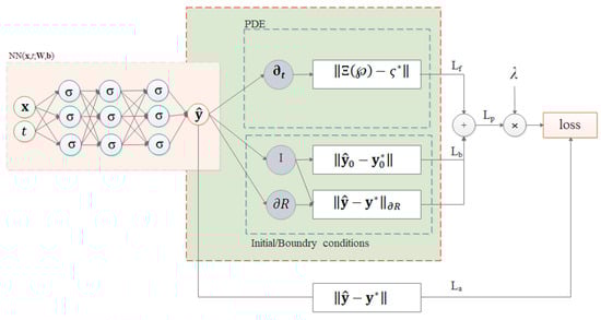
Figure 1.
PINN schematic algorithm for loss function.
Although the PINNs can introduce several differential equations in the loss function, the calculation of these equations significantly increases the computational burden of the training stage. To mitigate this problem, two novel architectures are proposed that can be applied to the space-discretized PDE. In this study, the EEM was used to discretize the governing PDE. In the first layout illustrated in Figure 2, parallel PINNs are trained simultaneously. These PINNs are connected to each other via the total loss function. The efficiency of the parallel PINNs is specifically important for complex and real-time systems in which analysis time is crucial. The proposed layout can be said to be more suitable for running it on GPUs, which significantly reduces the computational time. Besides, due to the independence of the PINNs in the parallel layout, the architecture of each PINN can be different from the rest, making the total layout of the framework more flexible. In some dynamic systems, one or two modes might be dominant and can play an important role in the system’s global behavior. One can reflect this priority by introducing a weighting parameter to the output of each PINN. Another solution is to focus on the dominant modes first and later use the estimated properties in the next modes. This framework shapes series PINNs, as demonstrated in Figure 3. In this regard, the importance of each mode is defined by the framework by order of the relative PINN in the framework. Also, one can terminate these series and control the output accuracy. Unlike the previous layout, the output of each PINN is necessary for subsequent PINNs. However, by placing the dominant modes in the early sector of the sequential framework, the subsequent PINNs benefit from previous estimates and run faster. It should be highlighted that, for generalizability purposes, one can estimate the structural properties, such as stiffness change, by introducing the proper physics-based equations and employing the PINN method. This can potentially be used for SHM of infrastructure systems subjected to unknown moving loads.
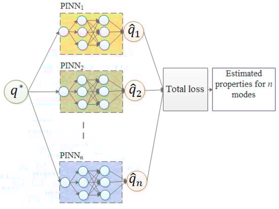
Figure 2.
Schematic framework with parallel PINNs.
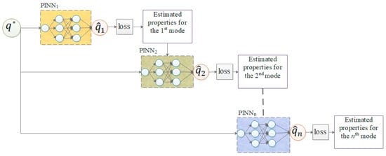
Figure 3.
Schematic framework with sequential PINNs.
2.2.1. PINN for ODE
Since introducing the physical equation in the PINN is essential, the equations and loss function are briefly reviewed for ODE and PDE. The dynamic equation for an SDOF is a classic example of ODEs. Consider an SDOF dynamic system where the mass and stiffness of the system are and , respectively. A viscous damper, , is added to the system to study the performance of the PINNs in tracking the vibration behavior of damping systems. The following equation represents the state-space equation for this system
where
Additionally, the measurement vector is defined as
and correspond displacement and acceleration observation variables. Now that the physical equation and measurement vector are defined, one can simply use Equation (9) as the loss function.
2.2.2. PINN for PDE
In this section, the vibration equation for a continuous beam is studied as a PDE. Consider a simply supported beam, where and are mass per unit length and flexural rigidity of the beam, and is the damping of the beam. The forced vibration equation of this system can be written as follows:
where denotes vertical displacement. By applying the EEM, the beam response is decoupled as
and are the modal shape and coordinate of the mode, respectively. By substituting Equation (14) in Equation (13), the modal equation results:
where,
and are the influence matrix and time history of the imposed force, respectively. Subsequently, the state-space equation for a beam subjected to a moving load is
where
In this formulation, is the modal matrix, and are the mass and changing position of the moving loads, respectively. Also, the measured vector, , is defined as:
where and are the correspondent displacement and acceleration observation matrix.
Since Equation (17) is composed of independent equations, it is proposed to consider an individual PINN for each equation which can be calculated in parallel or in series. In this regard, the global architecture will be more flexible since the local architecture of each equation is independent and can be adjusted to the physical equation properly. Figure 4 demonstrates the schematic layout of the proposed framework for a beam subjected to a moving load. It can estimate the state of the system and identify the system properties. In addition, the properties of the input load, the weight, and the velocity of the moving object, which has a key role in the control of the structures, can be determined through the framework of this study. The proposed algorithm for both sequential and parallel PINNs is introduced in Algorithm 1. In these algorithms, it is supposed that the noisy measurements of sensors are fed to the framework after discretization to modes by the EEM. Each layout consists of PINNs that work together.
| Algorithm 1 Proposed framewoark with sequential and parallel PINNs. |
| Input: and . |
 |
| Output: [state estimation; dynamic system properties; input load]. |
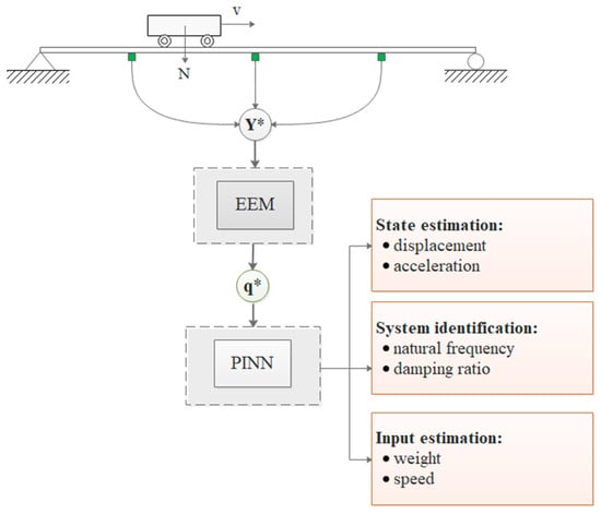
Figure 4.
Input and outputs of a PINN framework for a beam subjected to moving load.
3. Demonstrative Examples
The main purpose of this section is to evaluate the performance of the PINN in dynamic structural system identification and input force estimation. To evaluate the performance of PINN for dynamic structural system identification, two types of dynamic systems were considered for verification purposes: a linear Single Degree of Freedom (SDOF) system as well as a Pure Cubic Oscillator (PCO) as ODE examples; afterward, a simply supported beam as a bridge-type structure representing PDE problems were analyzed. In the last step, the capability of the PINN in estimating input force was examined by introducing a moving load to the bridge-type system.
To evaluate the performance of the PINN in determining the dynamic structural system identification, each system was trained for a short period of time with a few displacements and/or accelerations sensor outputs. By imposing physics equations constraints, both dynamic parameters and the state of the system were estimated. The accuracy of parameter estimations was investigated with different sensor noise levels, and the PINN and ANN’s capability in predicting the structure’s state was compared. Finally, the competency of the PINN in estimating input force was examined. In this regard, the weight and speed of a moving load were identified for a bridge-type structure. An overview of the demonstrative examples and their results is presented in Figure 5.
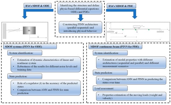
Figure 5.
The workflow of the paper and demonstrative examples.
3.1. SDOF System
The vibration of an SDOF system is a classical problem in the field of structural dynamics, and an analytical solution to this system is available. By assuming circular frequency,, and damping ratio,, as known parameters, the analytical response of the systems with is obtained:
where .
As discussed earlier, Equation (10) is regarded as a physics constraint for the PINN, and the outputs of the PINN are both dynamic properties of the SDOF and state prediction. In other words, the only input of the PINN is the state (displacement and/or acceleration) of the SDOF during the training period, , and the PINN will estimate the SDOF’s displacement and acceleration after the training period and also predict the system properties, . Here below, the inputs and outputs of PINN are laid out:
where is the number of samples in the training data, which in this case is the total time steps used for the training period. Now that the input and output of the PINN are known, the loss function is calculated:
represents the PINN estimation of the studied SDOF displacement at the time step; and are the unknown parameter; therefore, the PINN is expected to predict these parameters after training. In order to compare the accuracy of the predicted state of the PINN and the ANN, and were introduced to the model, respectively. Aiming for an accurate comparison, an identical architecture is considered for the analysis of both PINN and ANN. Since the behavior of the SDOF is not complex, a NN with one hidden layer with 50 nodes is selected for this section. It is noteworthy that the initial condition of the system, here , can also be introduced to the loss function. This criterion helps the PINN to converge numerically faster. However, since the initial condition might be unknown, it was not introduced to the presented models.
3.1.1. System Identification
In the first step, the capability of the PINN in system identification is evaluated. Since the ANN is not capable of parameter prediction, only the PINN’s estimates are presented in this section. To train the PINN, the analytical displacement of the SDOF was contaminated with an additive zero-mean white Gaussian noise which its Root Mean Square (RMS) was 1% of the RMS of the signal, and it was fed into the PINN during three natural periods. The performance of the PINN in the system identification framework was evaluated for various SDOF systems. Table 1 presents the predicted dynamic characteristics of different SDOFs. With a relative error of almost less than 1.5%, the results confirmed the accuracy of the estimated parameters. The relative error provides a normalized measure of the error in the estimated value. It is expressed as a ratio of the absolute error to the true or actual value. This accuracy level reduces with increasing damping ratios and amplification of the diminution effect, although the overall estimations can be said to be accurate. Eventually, a specific SDOF with a circular natural frequency of and a damping ratio of 0.005 was chosen for further studies.

Table 1.
Estimation of the PINN for dynamic characteristics.
The efficiency of NNs relies on both the quantity and quality of the training data. In the next step, the capability of the PINN for system identification was assessed for different training periods and noise levels subjected to the various initial conditions.
To evaluate the performance of the PINN with different training periods, the accuracy of the parameter estimation after (a) half, (b) two, and (c) three natural periods of training with different initial conditions are compared in Figure 6. The PINN can estimate the system properties accurately with less than half of the natural period, and by increasing the training time, the estimations become more precise. In order to evaluate the sensitivity of the PINN to the noise levels, the analyses were repeated for different input data with noise levels ranging from 1% up to 10% RMS of the training data. Based on Figure 7, the dynamic properties of the SDOF were estimated accurately for all noise levels. Despite increasing the noise level, the accuracy of the predicted parameters decreased as expectedly. These results are valid for different initial conditions.
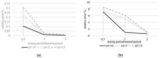
Figure 6.
PINN’s relative error with different training periods for (a) natural circular frequency; (b) damping ratio estimations.
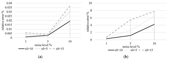
Figure 7.
PINN’s relative error with different noise levels for (a) natural circular frequency; (b) damping ratio estimations.
3.1.2. State Estimation
In this section, the accuracy of the predicted states during and after the training period is unveiled in detail. Figure 8 and Figure 9 represent the state estimation of the SDOF trained by displacement and acceleration measurements during three periods, respectively. Even though both PINNs estimations are accurate for the early training steps, the estimation error increases over time. It should be noted that for the system with acceleration training, Figure 9, the PINN needs to estimate the displacement by dealing with a more complicated process, double integration, and more time-consuming compared to the system trained by the displacement, Figure 8. Unlike integration operations, the derivation operations are calculated automatically during the training process. However, the results of this system are precise for both displacement and acceleration estimates. Figure 10 shows the loss function for a PINN that was trained on both displacement and acceleration inputs. As mentioned earlier, the loss function in PINNs consists of two components: La, data-driven term, and Lp, differential equation term. In Figure 10, these terms, in addition to the total loss function, are presented; while the physics equation term decreases to lower loss values, the data-driven term values of the displacement and acceleration increased to 0.007 and 0.02, respectively.
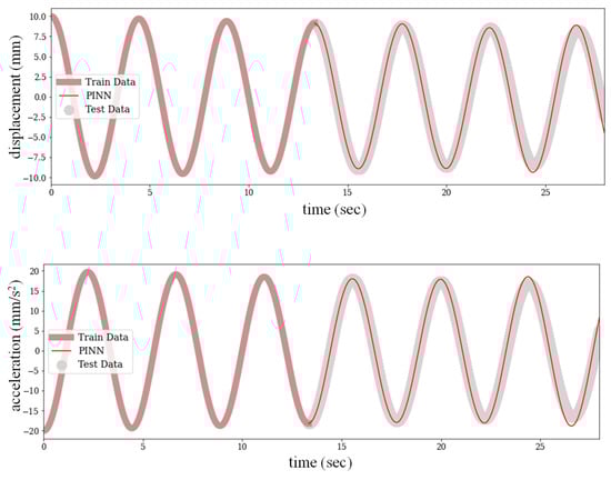
Figure 8.
Displacement and acceleration estimation of the SDOF trained by displacement measurements.
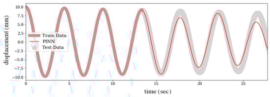
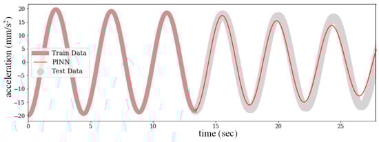
Figure 9.
Displacement and acceleration estimation of the SDOF trained by acceleration measurements.
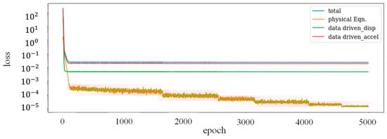
Figure 10.
PINN loss function with three periods of training by displacement and acceleration input.
To be able to dig more into the performance of the PINN during the training period, Figure 11 is plotted to represent the output of the PINN for these two constraints: consistency with the training data (displacement and acceleration) and satisfaction of the physical equation during the training period. It is evident that the output of the PINN for training data is accurate, but there is an error of about 2% in the physical equation constraint that reduces over the duration of analyses.
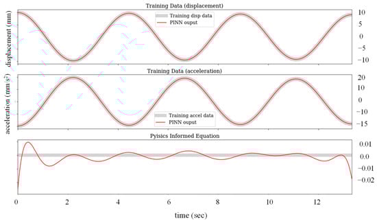
Figure 11.
Constraint satisfaction of the PINN during three natural periods of training: (top) input data consistency with estimated displacement; (middle) estimated acceleration; (bottom) physics equation satisfaction 0*.
In the last part of this section, the role of as the physics-informed regulator is explained. Based on the results of the system identification, the PINN can estimate the parameters of the physics equation precisely, but according to Figure 10, the data-driven phrases decrease rapidly to a specific value. By recalling Equation (9), it is reminded that plays an important role in deciding on the contribution of the physics equation to the final loss function. By increasing , the PINN is more strictly forced to follow the physics equation, while decreasing the gives more credibility to the measured data. In the extreme case of , the PINN turns into a conventional ANN, which only relies on the data during the training period. Figure 12 and Figure 13 present the estimated displacement and acceleration of the SDOF for the test periods, which is three times longer than the training period. It is obvious from both figures that the ANN cannot represent reliable estimation for long periods, whereas the PINN estimations are capable of following the main trend in all cases. All NNs show an acceptable state estimation for a short period after the training; however, there is an increasing discrepancy over time, which is more evident in the case of using lower λ. In fact, by increasing the λ, the PINN is more restricted to satisfy the physical equation, but it should be noted that this is true when the physics equation is reliable. In other words, the λ helps the PINN to regulate its prediction based on the relative reliability of the measured data and the physics equation.
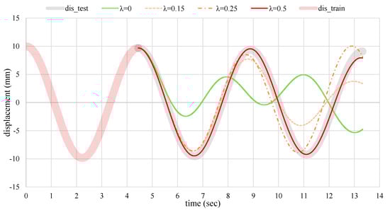
Figure 12.
Displacement estimation of the PINN for various λ and the ANN with λ = 0 during the test period.
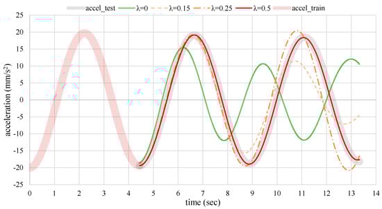
Figure 13.
Acceleration estimation of the PINN for various λ and the ANN with λ = 0 during the test period.
3.2. Pure Cubic Oscillator (PCO)
Due to the inherent complexity of nonlinear dynamic systems, these problems are often examined through the discretization and linearization of the nonlinear system. Therefore, in most cases, numerical methods are used to find the response of the nonlinear systems. The Duffing-type oscillators are a special case with nonlinear behavior and analytical solution. These oscillators are usually implemented in the nonlinear vibration absorbers [35]. In this study, the pure cubic oscillator, as a special case of the hardening duffing oscillators, is studied. The vibration equation of the PCO plotted in Figure 14 is described as
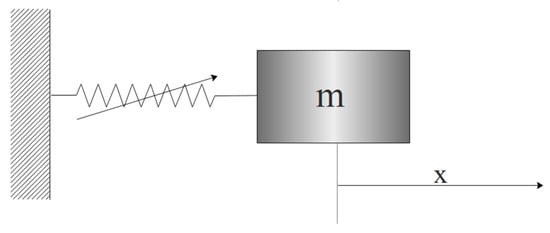
Figure 14.
Schematic representation for a nonlinear dynamic system.
The analytical solution of this system is governed by the elliptical function; hence, for a system with an initial displacement of the and zero initial velocity, one can find [36]
where is the Jacobi elliptic function; , elliptic parameter equals 0.5, and the parameter proportional to frequency is
It is worth mentioning that, unlike linear systems, the frequency is amplitude-dependent, and its amplitude dependency makes the influence of the initial condition more critical.
To explore the performance of the NNs, the vibration of a PCO with an initial displacement was studied. The displacement of the system during the two cycles was measured and fed to the NNs. The properties of the examined PCO for different properties and initial conditions are presented in Table 2. It confirms the accuracy of the estimated parameter with less than 0.1% error. Considering the complex nature of nonlinear systems, the superiority of the PINN over ANN in state estimation is evident. According to Figure 15, the PINN estimates the states accurately while the ANN fails to deliver acceptable estimations; this incompatibility increases over time. Based on Figure 16, during the training procedure, the PINN is obligated to simultaneously comply with the dynamic equation and measure displacement, which helps it to represent more accurate predictions and better parameter estimation (Table 2). The PINN satisfies Equation (22) as the physical constraint with an accuracy of less than 1%. In fact, the added constraint for the PINN clearly improves the training performance, as displayed in Figure 17. By comparing the loss function of the PINN and ANN during the training process, which is presented in Figure 17 and Figure 18, respectively, one can find out that, unlike the PINN, which shows a decreasing trend over epoch incrementation, the ANN shows a drastic decrease during the first epochs and stay stationary for the rest of the training. Although the fluctuations of the loss function decrease over time for both NNs, the total loss function of both NNs descends to 0.0001 at the end.
Table 2.
Estimation of the PINN for the nonlinear parameter.
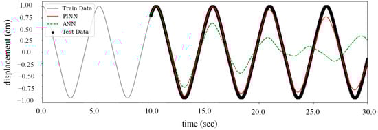
Figure 15.
The PINN and ANN state estimation for the test period after two natural training periods.
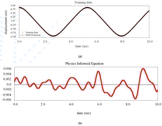
Figure 16.
Physic equation satisfaction of the PINN during two natural training periods: (a) input data consistency; (b) physics equation satisfaction 0*.
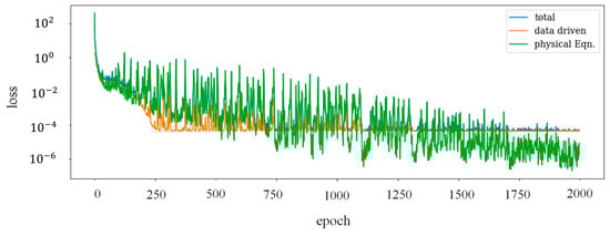
Figure 17.
Loss function of the PINN.
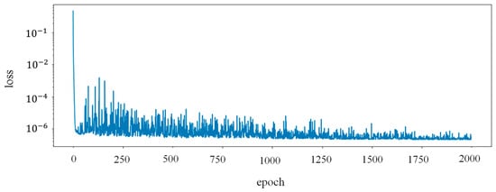
Figure 18.
Loss function of the ANN.
3.3. Simply Supported Beam
In this section, the efficiency of the proposed method is evaluated for bridge-type structures via analysis of a simply supported beam. To investigate the performance of the PINN in system identification and input estimation of the bridge-type structures, at first, the efficiency of the parallel and sequential PINNs in both system identification and state estimation was probed. Subsequently, the effectiveness of the proposed framework in the dynamic identification of beams subjected to moving load was unveiled.
The geometrical and dynamic properties of the studied beam are length m, mass per unit kg/m, flexural rigidity EI = 5 × 10⁻³N × m2, and modal damping coefficient ζ = 0.005 kN.s/m. In this study, three and six modes were considered in the reduced order model for the calculation of sensor outputs and NN’s analysis, respectively. It is assumed that three displacement sensors were installed at equal distances on the beam, as illustrated in Figure 19. The output of these sensors with a 1% RMS noise level is plotted in Figure 20.
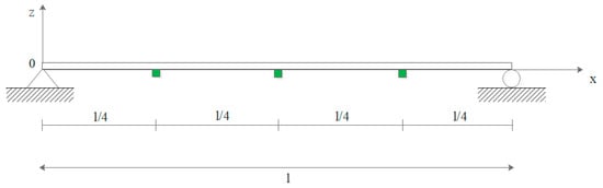
Figure 19.
Simply supported beam and sensor locations.
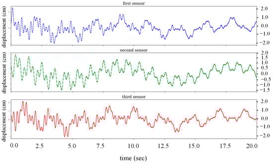
Figure 20.
Sensor outputs of the beam.
To introduce the set of ODEs into the PINNs, three parallel NNs with 200 nodes and two hidden layers were considered; three sets of equations were introduced to the PINN to connect these NNs. The loss function, which was used in the training procedure of the proposed PINN framework, is presented in Equation (25).
Figure 21 plots the modal predictions for the test period, where the PINN outperforms the ANN. The ANN shows an increasing time lag in the first mode and instability in the third mode. Unlike the ANN, the PINN presents acceptable predictions, especially for the first mode. Based on Figure 22, the ANN cannot deliver the phase lag for sensors and shows inconsistency.
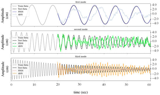
Figure 21.
PINN and ANN modal estimation with two hidden layers for the test period.
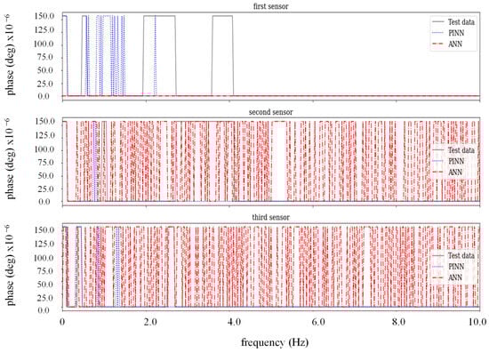
Figure 22.
PINN and ANN phase lag of each sensor with two hidden layers for the test period.
To make the architecture of the NNs more efficient, three different architectures were considered for each mode based on the mode’s specific attributes. Since the first mode experienced fewer oscillations due to lower vibration frequency, only one layer with 200 nodes was suggested for both NNs architectures, whereas for the next two modes with higher frequencies, three and five layers were introduced for the second and third modes, respectively. The effect of this modification is obvious in both precise circular frequency estimation in Table 3 and state estimations for the next steps in Figure 23. On the other hand, according to Figure 24, the ANN shows a more stable estimation for the second and third modes, but modal predictions deviate from their course over time. The results of the FFT analysis on both the PINN and the ANN state estimations are illustrated in Figure 25, demonstrating that, unlike the PINN, ANN cannot track the higher frequencies precisely, which results in poor modal and, thereafter, state estimations.
Table 3.
Estimation of PINN for the first three modal dynamic characteristics.
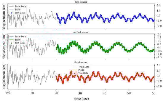
Figure 23.
PINN state estimation with modified hidden layers for the test period.
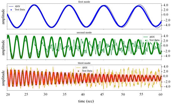
Figure 24.
ANN modal estimation with modified hidden layers for the test period.
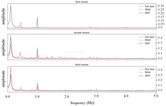
Figure 25.
FFT analysis on the PINN and ANN state estimations with modified hidden layers for the test period.
Finally, to evaluate the generalizability of the NNs results on the other points of the beam, the state estimations of both PINN and ANN for two checkpoints are examined. According to Figure 26, the PINN shows accurate estimations for these two points; however, there is a minor lag at the end of the test period. This issue affects the ANN results more seriously; thus, the ANN’s predictions are accurate for a much shorter time.
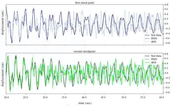
Figure 26.
PINN and ANN state estimation at the checkpoints with modified hidden layers for the test period.
3.3.1. Beam Subjected to Moving Load
To examine the applicability of the proposed method for the identification of structural parameters of the beam subjected to moving loads, it is assumed that four moving loads, which weigh 0.05 kg/vehicle each, are passing the beam with equal distances, = 0.2 m with a constant velocity, = 0.125 m/s, which is 1.9 times higher than the critical velocity. After departing the last moving load, the beam experiences a free vibration phase, which is the desired time window for extracting the beam properties. It is assumed that three displacement/acceleration sensors, which are indicated with solid green rectangles, are installed on the beam at the middle point between the vehicles, as shown in Figure 27. The output of these sensors is contaminated with a 1% RMS noise level. Figure 28 shows the output of the third accelerometer.
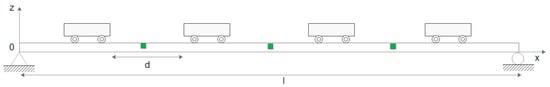
Figure 27.
A simply supported beam subjected to moving inertial loads with a single span.
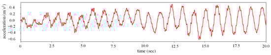
Figure 28.
The output of the third accelerometer.
After the departure of the last moving load, the beam experiences a free vibration phase. During this phase, the properties of the beam are evaluated by the PINN. In the first step, NNs with three hidden layers and 200 nodes are considered. Since the first two modes are more important, two parallel NNs are considered to calculate the properties of the first two modes. This layout was presented in the previous section in Figure 2. These two NNs are connected through the modal equation of the first two modes, as explained in Equation (25). In Figure 29, the loss function of two modal equations in comparison to the displacement sensor outputs are plotted. While the first modal equation descends to lower loss values, the second modal equation experiences more fluctuations. Table 4 shows the predicted modal properties of the beam. Although the proposed architecture precisely predicts the damping ratio and the first natural frequency, the error is noticeably slight in the second natural frequency estimation. Figure 30 confirms these results.
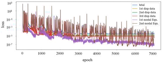
Figure 29.
The loss function of the parallel PINNs with displacement input.
Table 4.
The modal properties of the beam subjected to moving loads estimated by the PINN.
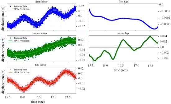
Figure 30.
Parallel PINN estimations during the training period with displacement output.
In the second layout, a sequential architecture for the PINNs was considered. Since the first mode plays an important role in the displacement estimation of the beam, for the first phase, only one PINN with three hidden layers and 50 nodes is defined; therefore, only the first modal equation was considered in the loss function. In this regard, the first natural frequency, ω1, and the damping ratio, ζ, are estimated and then fed into the next series of the PINNs. In the next step, since the properties of the first modal equations were already estimated, only the second natural frequency needs to be predicted. In a sequential layout, each step needs less calculation and therefore runs faster; it relies on the results of the previous phase. This series can also be adjusted to the desired accuracy. For instance, when only the first natural frequency plays a key role, running the next PINNs is not necessary, and the sequence can be terminated based on the desired accuracy. Once again, it is reminded that this layout is essential for situations in which specific modes contribute more to the results than the other modes. For instance, in cases with accelerometer inputs, the parallel layout is more accurate in modal frequencies and damping ratio estimations. Based on Figure 31, the sequential layout satisfies all constraints during the training period, and the parallel PINN can outperform the series layout predictions. In conclusion, both layouts represent acceptable estimations, but the input of the PINN affects the efficiency of these two layouts.
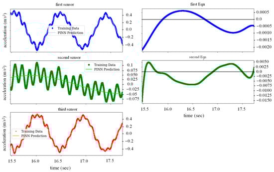
Figure 31.
Sequential PINN estimations during the training period with acceleration input.
3.3.2. Force Identification of Moving Load
In the last section, the accuracy of the PINN in estimating a moving load is studied. In this regard, the properties of the beam are assumed to be known, either by the proposed algorithm from previous sections or other methods; hence, the weight and velocity of the moving load are considered unknown parameters. It should be noted that the PINN is trained by the sensor outputs during the moving load passage.
Consider a simply supported beam, the same as in the previous section that is subjected to a moving load (Figure 32). Supposing the forced movement initiates at and has a constant velocity of , the implied force is calculated as
where is the mass of the moving load, is the gravity acceleration, and is the Dirac delta function. By transforming the applied force to the modal force, one gets
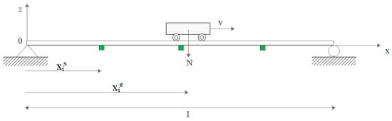
Figure 32.
Model of the moving load passing a simply supported beam.
In this section, the PINN is informed by only the first two modes. In other words, the first two modal equations are introduced to the PINN. In addition, the outputs of three sensors during load passage are used for PINN training. The loss function of this system for mass and velocity identification is
To examine the performance of the PINN with different input load predictions, moving loads with various weights and velocities were applied to the proposed model. Figure 33 demonstrates the accuracy of the estimated weight and velocity for the PINN that was trained with three displacement sensors with a 1% RMS noise level. In both cases, the relative error is less than 0.1%, which affirms the PINN capability in predicting moving loads. In addition, it is inferred that by increasing the velocity of the moving load, the estimation accuracy decreases. This is because, by increasing velocity, the time that moving load passes on the beam reduces, and inevitably the time window for gathering data and training the PINN reduces. On the contrary, by increasing the weight of the moving load, the beam experiences more distinct deflections; therefore, the accuracy of the weight estimation increases by incrementing the weight of the load. Based on Figure 34, the accelerometer outputs help the PINN estimate the weight as accurately as the displacement sensors; however, the PINN with acceleration inputs fails to accurately estimate higher velocities. It is worth mentioning that, unlike the displacement sensors, the acceleration inputs make the training of the PINN more challenging and time-consuming. Once again, it is reminded that in contrast to displacement inputs, the acceleration inputs fluctuate more intensely during the passage of the moving load. Also, as mentioned in the previous sections, the process of training the PINNs with acceleration entails integration operations which, unlike the differential operation, brings more complexity to the training process.
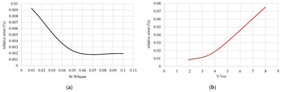
Figure 33.
Moving load estimations using displacement sensors: (a) weight; (b) velocity estimation of the moving load.
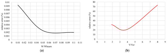
Figure 34.
Moving load estimations using accelerometer sensors: (a) weight; (b) velocity estimation of the moving load.
4. Conclusions
Within the scope of this study, the two novel architectures were proposed to employ the PINNs in the dynamic system identification and moving load assessment. The proposed architectures were applied to real-time structural system identification and input estimation. The presented methods were validated using simulated experiments on different dynamic systems with various levels of complexity.
In the first step, to elaborate on the details and capability of the PINN framework for system identification and state prediction, the linear and nonlinear SDOFs were studied, respectively. In this regard, various measurement scenarios with different noise levels and training periods were applied to evaluate the performance of the PINN in system identification. Based on the results, the proposed PINN framework can estimate the natural frequency and damping ratio even when the high noise level is 10% RMS. Although the PINN can predict the dynamic properties of the SDOFs with half of the natural period training, it is recommended to train the model at least for one natural period to obtain more accurate results. The capability of the PINN in state estimation was compared to the ANNs, and the superiority of the PINN frameworks was confirmed. The role of as the physics-informed regulator was studied, and it was shown that by increasing the from 0 to 0.5, the model could predict the state of the system for almost four times longer period, which highlights the significance of taking into account prior physical knowledge in the structure of the PINNs.
In the next step, the bridge-type structure was chosen to demonstrate the efficacy of the PINNs in system identification and load assessment of the beams subjected to the moving loads. The importance of the NNs architectures was assessed via various numerical analyses. It was shown that by modifying the hidden layers of the PINN, one could considerably improve the accuracy of the estimated parameters. Furthermore, the competency of the PINN frameworks for both parallel and sequential architectures was studied. The findings show that both architectures can estimate the modal properties of the beam accurately; although the parallel PINNs need less computation time, making them a better choice for more complex systems. For load assessment of the moving forces specifically important in the realm of bridge design and construction, it has been shown that using both accelerometer and displacement sensor measurements, the proposed framework delivers reliable and robust results for estimating the weight of the moving load. However, for velocity estimation of the moving load, it is recommended to use displacement measurements for training the PINNs.
The following results can be drawn based on the conducted study through extensive numerical examples;
- The PINN architectures in the published literature do not properly address the integration of structural dynamics PDEs into NN objective function. Nevertheless, the novel architecture proposed herein utilizes parallel and sequential PINNs successfully.
- The proposed parallel layout enables the PINN framework to accurately identify the properties of the continuous systems and moving loads. This is an important step toward the generalization of the PINN framework for developing an accurate model of continuous structures and, more specifically, systems subjected to moving loads, such as bridges;
- Unlike conventional ANNs, the novel PINN architectures feature excellent generalizability when applied to output-only system identification of dynamic structural systems. This makes them suitable candidates for operational system identification, where one needs to simultaneously consider input, model, and measurement uncertainties.
Author Contributions
Conceptualization, S.M. and S.E.A.; methodology, S.M. and S.E.A.; software, S.M. and B.D.; validation, S.M. and B.D.; formal analysis, S.M.; investigation, S.M., B.D., S.E.A. and M.M.; resources, S.E.A. and M.M.; visualization, S.M. and B.D.; supervision, S.E.A. and M.M. All authors have read and agreed to the published version of the manuscript.
Funding
This research received no external funding.
Data Availability Statement
Not applicable.
Conflicts of Interest
The authors declare no conflict of interest.
References
- Hossain, M.S.; Ong, Z.C.; Ismail, Z.; Noroozi, S.; Khoo, S.Y. Artificial neural networks for vibration based inverse parametric identifications: A review. Appl. Soft Comput. J. 2017, 52, 203–219. [Google Scholar] [CrossRef]
- De Souza, C.P.G.; Kurka, P.R.G.; Lins, R.G.; de Araújo, J.M. Performance comparison of non-adaptive and adaptive optimization algorithms for artificial neural network training applied to damage diagnosis in civil structures. Appl. Soft Comput. 2021, 104, 107254. [Google Scholar] [CrossRef]
- Le Riche, R.; Gualandris, D.; Thomas, J.J.; Hemez, F. Neural Identification of Non-linear Dynamic Structures. J. Sound Vib. 2001, 248, 247–265. [Google Scholar] [CrossRef]
- Xu, B.; Wu, Z.; Chen, G.; Yokoyama, K. Direct identification of structural parameters from dynamic responses with neural networks. Eng. Appl. Artif. Intell. 2004, 17, 931–943. [Google Scholar] [CrossRef]
- Facchini, L.; Betti, M.; Biagini, P. Neural network based modal identification of structural systems through output-only measurement. Comput. Struct. 2014, 138, 183–194. [Google Scholar] [CrossRef]
- Liu, D.; Tang, Z.; Bao, Y.; Li, H. Machine-learning-based methods for output-only structural modal identification. Struct. Control. Health Monit. 2021, 28, 1–22. [Google Scholar] [CrossRef]
- Liang, Y.C.; Feng, D.P.; Cooper, J.E. Identification of restoring forces in non-linear vibration systems using fuzzy adaptive neural networks. J. Sound Vib. 2001, 242, 47–58. [Google Scholar] [CrossRef]
- Dudek, G. A constructive approach to data-driven randomized learning for feedforward neural networks. Appl. Soft Comput. 2021, 112, 107797. [Google Scholar] [CrossRef]
- Khanmirza, E.; Khaji, N.; Khanmirza, E. Identification of linear and non-linear physical parameters of multistory shear buildings using artificial neural network. Inverse Probl. Sci. Eng. 2015, 23, 670–687. [Google Scholar] [CrossRef]
- Xie, S.L.; Zhang, Y.H.; Chen, C.H.; Zhang, X.N. Identification of nonlinear hysteretic systems by artificial neural network. Mech. Syst. Signal Process. 2013, 34, 76–87. [Google Scholar] [CrossRef]
- Liu, Z.; Fang, H.; Xu, J. Identification of piecewise linear dynamical systems using physically-interpretable neural-fuzzy networks: Methods and applications to origami structures. Neural Netw. 2019, 116, 74–87. [Google Scholar] [CrossRef] [PubMed]
- Wang, Q.; Wu, D.; Tin-Loi, F.; Gao, W. Machine learning aided stochastic structural free vibration analysis for functionally graded bar-type structures. Thin-Walled Struct. 2019, 144, 106315. [Google Scholar] [CrossRef]
- Yazdizadeh, A.; Khorasani, K.; Patel, R.V. Identification of a two-link flexible manipulator using adaptive time delay neural networks. IEEE Trans. Syst. Man Cybern. Part B 2000, 30, 165–172. [Google Scholar] [CrossRef] [PubMed]
- Deng, J. Dynamic neural networks with hybrid structures for nonlinear system identification. Eng. Appl. Artif. Intell. 2013, 26, 281–292. [Google Scholar] [CrossRef]
- Raissi, M.; Perdikaris, P.; Karniadakis, G.E. Physics informed deep learning (Part II): Data-driven discovery of nonlinear partial differential equations. arXiv 2017. [Google Scholar]
- Raissi, M.; Perdikaris, P.; Karniadakis, G.E. Physics informed deep learning (Part I): Data-driven discovery of nonlinear partial differential equations. arXiv 2017, arXiv:1711.10561. [Google Scholar]
- Jin, X.; Cai, S.; Li, H.; Karniadakis, G.E. NSFnets (Navier-Stokes flow nets): Physics-informed neural networks for the incompressible Navier-Stokes equations. J. Comput. Phys. 2021, 426, 109951. [Google Scholar] [CrossRef]
- Jiang, C.; Vinuesa, R.; Chen, R.; Mi, J.; Laima, S.; Li, H. An interpretable framework of data-driven turbulence modeling using deep neural networks. Phys. Fluids 2021, 33, 055133. [Google Scholar] [CrossRef]
- Haghighat, E.; Raissi, M.; Moure, A.; Gomez, H.; Juanes, R. A physics-informed deep learning framework for inversion and surrogate modeling in solid mechanics. Comput. Methods Appl. Mech. Eng. 2021, 379, 113741. [Google Scholar] [CrossRef]
- Azam, S.E.; Rageh, A.; Linzell, D. Damage detection in structural systems utilizing artificial neural networks and proper orthogonal decomposition. Struct. Control Health Monit. 2019, 26, 1–24. [Google Scholar] [CrossRef]
- Jain, J.; Kundra, T. Model based online diagnosis of unbalance and transverse fatigue crack in rotor systems. Mech. Res. Commun. 2004, 31, 557–568. [Google Scholar] [CrossRef]
- Nascimento, R.G.; Fricke, K.; Viana, F.A.C. A tutorial on solving ordinary differential equations using Python and hybrid physics-informed neural network. Eng. Appl. Artif. Intell. 2020, 96, 103996. [Google Scholar] [CrossRef]
- Haghighat, E.; Juanes, R. SciANN: A Keras/TensorFlow wrapper for scientific computations and physics-informed deep learning using artificial neural networks. Comput. Methods Appl. Mech. Eng. 2021, 373, 113552. [Google Scholar] [CrossRef]
- Haghighat, E.; Raissi, M.; Moure, A.; Gomez, H.; Juanes, R. A deep learning framework for solution and discovery in solid mechanics. arXiv 2020, arXiv:2003.02751. [Google Scholar]
- Jagtap, A.D.; Kharazmi, E.; Karniadakis, G.E. Conservative physics-informed neural networks on discrete domains for conservation laws: Applications to forward and inverse problems. Comput. Methods Appl. Mech. Eng. 2020, 365, 113028. [Google Scholar] [CrossRef]
- Kharazmi, E.; Zhang, Z.; Karniadakis, G.E.M. VPINNs: Variational physics-informed neural networks for solving partial differential equations. arXiv 2019, arXiv:1912.00873. [Google Scholar]
- Kharazmi, E.; Zhang, Z.; Karniadakis, G.E.M. hp-VPINNs: Variational physics-informed neural networks with domain decomposition. Comput. Methods Appl. Mech. Eng. 2021, 374, 113547. [Google Scholar] [CrossRef]
- Haghighat, E.; Bekar, A.C.; Madenci, E.; Juanes, R. Deep learning for solution and inversion of structural mechanics and vibrations. In Modeling and Computation in Vibration Problems, Volume 2: Soft Computing and Uncertainty; IOP Publishing: Bristol, UK, 2021; pp. 1–18. [Google Scholar]
- Goswami, S.; Anitescu, C.; Chakraborty, S.; Rabczuk, T. Transfer learning enhanced physics informed neural network for phase-field modeling of fracture. Theor. Appl. Fract. Mech. 2020, 106, 102447. [Google Scholar] [CrossRef]
- Zhang, E.; Yin, M.; Karniadakis, G.E. Physics-Informed Neural Networks for Nonhomogeneous Material Identification in Elasticity Imaging. arXiv 2020, arXiv:2009.04525. [Google Scholar]
- Lai, Z.; Mylonas, C.; Nagarajaiah, S.; Chatzi, E. Structural identification with physics-informed neural ordinary differential equations. J. Sound Vib. 2021, 508, 116196. [Google Scholar] [CrossRef]
- Adeli, H.; Yeh, C. Perceptron Learning in Engineering Design. Comput. Civ. Infrastruct. Eng. 1989, 4, 247–256. [Google Scholar] [CrossRef]
- Tiumentsev, Y.V.; Egorchev, M.V. Neural Network Black Box Approach to the Modeling and Control of Dynamical Systems. Neural Netw. Model. Identif. Dyn. Syst. 2019, 1, 93–129. [Google Scholar]
- Baydin, A.G.; Pearlmutter, B.A.; Radul, A.A.; Siskind, J.M. Automatic differentiation in machine learning: A survey. J. Mach. Learn. Res. 2018, 18, 1–43. [Google Scholar]
- Ding, H.; Chen, L.Q. Designs, analysis, and applications of nonlinear energy sinks. Nonlinear Dyn. 2020, 100, 3061–3107. [Google Scholar] [CrossRef]
- Kovacic, I. Nonlinear Oscillations; Springer International Publishing: Cham, Germany, 2020. [Google Scholar]


Disclaimer/Publisher’s Note: The statements, opinions and data contained in all publications are solely those of the individual author(s) and contributor(s) and not of MDPI and/or the editor(s). MDPI and/or the editor(s) disclaim responsibility for any injury to people or property resulting from any ideas, methods, instructions or products referred to in the content. |
© 2023 by the authors. Licensee MDPI, Basel, Switzerland. This article is an open access article distributed under the terms and conditions of the Creative Commons Attribution (CC BY) license (https://creativecommons.org/licenses/by/4.0/).