Machine Learning Method Based on Symbiotic Organism Search Algorithm for Thermal Load Prediction in Buildings

Abstract

This research investigates the efficacy of a proposed novel machine learning tool for the optimal simulation of building thermal load. By applying a symbiotic organism search (SOS) metaheuristic algorithm to a well-known model, namely an artificial neural network (ANN), a sophisticated optimizable methodology is developed for estimating heating load (H_L) in residential buildings. Moreover, the SOS is comparatively assessed with several identical optimizers, namely political optimizer, heap-based optimizer, Henry gas solubility optimization, atom search optimization, stochastic fractal search, and cuttlefish optimization algorithm. The dataset used for this study lists the H_L versus the corresponding building conditions and the model tries to disclose the nonlinear relationship between them. For each mode, an extensive trial and error effort revealed the most suitable configuration. Examining the accuracy of prediction showed that the SOS–ANN hybrid is a strong predictor as its results are in great harmony with expectations. Moreover, to verify the results of the SOS–ANN, it was compared with several benchmark models employed in this study, as well as in the earlier literature. This comparison revealed the superior accuracy of the suggested model. Hence, utilizing the SOS–ANN is highly recommended to energy-building experts for attaining an early estimation of the H_L from a designed building’s characteristics.

1. Introduction

The world has witnessed a considerable rise in energy consumption trends due to economic developments, population growth, and enhanced quality of living in recent decades [1,2]. Accordingly, the Global Energy & CO₂ Status Report indicates a doubled global energy consumption growth rate in 2018 relative to 2010 [3]. Hence, energy performance analysis is among the most important steps of construction planning [4,5]. It is crucial for the sustainable design of buildings and has a significant contribution to global conservation and environmentally protective policies [6]. Despite satisfying promises shown by different conventional methods (e.g., numerical [7], analytical [8], and statistical [9] approaches) for thermal behavior analysis, more sophisticated models such as artificial intelligence (AI) are attracting high attention.

Extending the application of state-of-the-art technology reveals that different inventions/developments have properly served in solving different engineering issues [10,11,12]. These developments comprise a wide variety of numerical [13], empirical [14], and experimental [15] approaches for dealing with a given problem. For instance, designing novel algorithms [16,17] toward facilitating (i.e., automation and acceleration of) time-consuming tasks has been the primary objective of engineering efforts such as safety analysis [18] and urban monitoring [19]. Recently, due to computational and coding progress, the prediction of complicated parameters has been investigated [20]. In this regard, experts have benefited from so-called machine learning techniques that can map intricate relationships in existing samples [21,22,23].

The energy management of a building is a complicated task because of the shifts in several contributive factors that can affect indoor conditions [24]. Such difficulties have encouraged engineers to change their tendency to use traditional time-consuming approaches toward soft computing models, such as machine learning, for simulating different energy-related parameters. The ability to explore nonlinear dependencies is regarded as the most notable advantage of machine learning models. In the case of energy efficiency analysis, engineers have benefited from models such as artificial neural networks (ANNs) [25,26] and support vector machines (SVMs) [27,28] for energy consumption in various building types. Fuzzy-based models are other popular approaches for dealing with energy prediction problems [29,30].

Going deeper into the literature, Ngo, et al. [31] proposed the use of an ensemble machine learning and compared it to ANN, SVM, and M5Rules predictors for 24 h energy consumption prediction. They observed very significant improvements (i.e., 123% error reduction) as a consequence of using an ensemble model. Elias and Issa [32] employed an ANN model for estimating the heating load (H_L) and cooling load (C_L) of single-family residences. They used a large dataset belonging to 18,000 new residences in Florida constructed in [2009, 2019]. The ANN was finally suggested as having the potential to assist designers of buildings. Jang, et al. [33] applied long- and short-term memory (LSTM) with different data scenarios for simulating heating energy consumption in nonresidential buildings. Zhou, et al. [34] introduced a combination of ensemble empirical mode decomposition with adaptive noise, autoregressive integrated moving average, and bi-directional LSTM for analyzing and predicting short-term H_L. The model achieved a good prediction with a root-mean-square error (RMSE) of 70.25 and a correlation of 0.983. Many similar applications can be found in earlier studies, such as [35,36,37].

The field of machine learning experienced significant advances by inventing metaheuristic algorithms. In general words, these algorithms are capable of optimizing complex problems [38]. Being able to synthesize with a generic machine learning model, metaheuristic algorithms can save them from weaknesses in computations such as local minima issues [39,40]. Compared with conventional methods, metaheuristic optimization performs much better in multiple aspects. Pachauri and Ahn [41] employed a regression tree ensemble for H_L and C_L estimation. The parameters of this model, however, were determined using a metaheuristic algorithm, namely shuffled frog leaping optimization. They reported a considerable improvement in the error of prediction of both thermal loads when the hybrid model was compared to benchmarks of stepwise regression and Gaussian process regression. The proposed model was lastly recommended to tune the performance of the heating, ventilation, and air conditioning (HVAC) system. Almutairi, et al. [42] combined an ANN with teaching–learning based optimization (TLBO) for predicting the H_L; with an RMSE value of 2.11 obtained for the TLBO–ANN versus 2.54, 2.70, and 2.27, the proposed model outperformed three benchmarks. In a comparative study, Xu, et al. [43] declared the superiority of biogeography-based optimization (BBO) over several similar metaheuristic techniques, especially traditional optimizers such as genetic algorithm and particle swarm optimization. Similar research can be found in studies by Moayedi and Mosavi [44], Guo, et al. [45], etc.

Taking a closer look at the metaheuristic-related works, especially in the energy efficiency domain, it can be inferred that the wide variety of these algorithms has led to occasional improvements in the optimal models found. Hence, it is necessary to keep the methodologies updated with the latest developments in metaheuristic techniques. This study introduces a novel hybrid model for predicting the H_L of residential buildings. A symbiotic organism search (SOS) algorithm is proposed for optimizing an ANN model to discover the pattern of H_L in relation to the building architecture. The SOS is a potential optimization technique that has been favorably used for training ANNs [46,47].

In addition to testing and introducing a new algorithm, another novelty of this work lies in an extensive comparative effort. The performance of the SOS is compared with six other techniques, namely political optimizer (PO), heap-based optimizer (HBO), Henry gas solubility optimization (HGSO), atom search optimization (ASO), stochastic fractal search (SFS), cuttlefish optimization algorithm (CFOA), which are, for the first time, used in this study, as well as several models assessed in earlier literature for the same purpose. The results would, therefore, highly assist energy and building experts by saving time and cost in selecting suitable models for energy performance approximation.

2. Materials and Methods

2.1. Data Provision

To obtain a proper understanding of the H_L using machine learning algorithms, the models need to recognize the parameter that is dependent on one or more conditioning factors (known as target and input factors). In other words, this dependency is mathematically mapped by the algorithms to create a pattern from the H_L behavior.

In this work, the target and input parameters are contained in a public dataset downloaded from UCI Machine Learning Repository (available on this webpage: https://archive.ics.uci.edu/ml/datasets/energy+efficiency accessed on 9 November 2022). This dataset was originally produced in research by Tsanas and Xifara [48] who gathered the simulation condition and the corresponding final thermal loads (in kWh/m²) of different residential buildings. Considering the input data of relative compactness (C_R), surface area (S_A), wall area (S_W), roof area (S_R), overall height (H_T), orientation (O), glazing area (S_G), and glazing area distribution (DS_G) and their variation, a total of 768 buildings were analyzed.

The buildings are characterized by a volume of 771.75 m³. Regarding the input parameters, the C_R of a place represents the ratio between the volume and the related area (here C_R = $\frac{6\times Volum{e}^{\frac{2}{3}}}{Area}$) and the S_G measures the total area (comprising frame, glazing, and sash) obtained from the rough opening. In this work, this parameter is stated by four ratios (including 0.0, 0.1, 0.25, and 0.4) relative to the whole floor area. Additionally, the DS_G expresses how these areas are distributed in the building of interest [49,50]. Possible scenarios considered for this factor are (a) no glazing, (b) giving 0.25 of glazing to each side, (c) giving 55% to the North and 15% to each of the other cardinal directions, (d) giving 55% to East and 15% to each of the other cardinal directions, (d) giving 55% to South and 15% to each of the other cardinal directions, and (e) giving 55% to West and 15% to each of the other cardinal directions [51,52]. Further details regarding the input parameters can be found in the reference paper [48].

Table 1. Statistical analysis of the constituent parameters.

Parameter	CR	SA	SW	SR	HT	O	SG	DSG	HL
Range	[0.6, 0.9]	[514.5, 808.5]	[245.0, 416.5]	[110.2, 220.5]	[3.5, 7.0]	[2.0, 5.0]	[0.0, 0.4]	[0.0, 5.0]	[6.01, 43.10]

expresses the range of values for the whole dataset. Moreover, Figure 1 depicts the scatter charts of each factor relative to the others. The values included in the correlation charts indicate the proportionality between the two parameters of interest. For instance, the correlation between the H_L and C_R is 0.62. Note that higher values indicate higher agreement in the behavior of the parameters and vice versa. According to these results, H_T and S_R with respective correlation values of 0.89 and −0.86 have the largest direct and adverse proportionality with the H_L; the histogram of the input and target factors is shown in this illustration.

The dataset is later divided into two subsets with 614 and 154 samples. These numbers stand for 80% and 20% of the whole, respectively. The aim of this division is to provide training and testing samples that are different from the other. The model uses the first dataset (training dataset with 80% of the whole) to learn and test its knowledge with the second dataset (testing dataset with 20% of the whole).

Important assessments of this dataset carried out in previous studies (e.g., by Zheng, et al. [53] and Wu, et al. [54]) indicate that the input factors should have sufficient importance for predicting the thermal loads. According to these studies, the inputs S_G and C_R have the greatest importance in this regard.

2.2. Assessment Formulas

The assessment of the results is handled by the three indicators of mean absolute error (MAE), the Pearson correlation index (R), and RMSE. Based on their formulation presented below, MAE and RMSE deal with the difference between the predicted and expected H_Ls, while the R index shows the correlation between these values. Equations (1)–(3) formulate the R, MAE, and RMSE in which N is the number of samples that are assessed (i.e., the size of the dataset).

$$R=\frac{{\displaystyle \sum _{i=1}^N(H_L{}_{i_{predicted}}-{\overline{H_L}}_{predicted})(H_L{}_{i_{\exp ected}}-{\overline{H_L}}_{\exp ected})}}{\sqrt{{\displaystyle \sum _{i=1}^N{(H_L{}_{i_{predicted}}-{\overline{H_L}}_{predicted})}^2}}\sqrt{{\displaystyle \sum _{i=1}^N{(H_L{}_{i_{\exp ected}}-{\overline{H_L}}_{\exp ected})}^2}}}$$

(1)

$$MAE=\frac{1}{N}{\displaystyle \sum _{i=1}^N|H_L{}_{i_{\exp ected}}-H_L{}_{i_{predicted}}|}$$

(2)

$$RMSE=\sqrt{\frac{1}{N}{{\displaystyle \sum _{i=1}^N[(H_L{}_{i_{\exp ected}}-H_L{}_{i_{predicted}})]}}^2}$$

(3)

2.3. Methodology

The SOS algorithm was proposed by Cheng and Prayogo [55]. This algorithm is a simulation of symbiotic interaction aimed at determining the best-fitting organism. The biological interaction of two organisms within the existing ecosystem is the essence of this algorithm, which is drawn on three phases, namely mutualism, commensalism, and parasitism.

In the first phase, with X_i as the organism corresponding to the ith individual in the ecosystem and X_j as a randomly chosen organism for interaction with X_i, a mutualistic relationship is formed toward enhancing the survival competency of these two organisms in the ecosystem. Equation 4 shows the process for making new candidate solutions:

$$X_{i\_new}=X_i+\gamma \left(X_b-MV\times B{F}_1\right)$$

(4)

$$X_{j\_new}=X_j+\mu \left(X_b-MV\times B{F}_2\right)$$

(5)

in which benefit factors are signified by $B{F}_1$ and $B{F}_2$ indicating partial and full benefit levels for the organisms. Additionally, $X_b$ stands for the largest adaption of organisms, $\gamma$ and $\mu$ are random values varying from 0 to 1, and $MV$ gives the mutual vector representing the characteristics between organisms.

In the commensalism phase, an X_j is randomly selected to interact with X_i. In this stage, it is assumed that X_i aims to take advantage of this interaction for gaining benefits, while the relationship is neither beneficial nor harmful for X_j. The new candidate solution corresponding to X_i is calculated as follows:

$$X_{i\_new}=X_i+\mathsf{\Delta }\left(X_b-X_j\right)$$

(6)

where $\mathsf{\Delta }$ randomly falls between −1 and 1. Based on the regulations of this algorithm, $X_{i\_new}$replaces the previous version if it provides a higher fitness.

In the third stage, i.e., parasitism, an artificial parasite vector is created since X_i acts like an anopheles mosquito. In this process, X_i is duplicated in the search space and the dimensions are updated using a random value. Additionally, X_j plays the role of host for the parasite vector. In the following, the fitness of both organisms is computed and the one having the lower fitness is eliminated [56,57].

2.4. Hybridization

Generally, a metaheuristic algorithm can play the role of optimizer for any viable problem [58]. It gives an optimum solution based on a maximized/minimized cost function. When it is applied to machine learning models, it aims to minimize the training error by providing the best computational configuration for the model. Taking ANN as an example, it optimizes the weights and biases that create a mathematical perception of the problem [59,60].

In order to develop a hybrid of ANN with any metaheuristic algorithm (here SOS), the below steps should be carried out:

(a)

Selection of an appropriate ANN structure;

(b)

Introduction of the determined ANN to the intended algorithm as the problem function to be optimized;

(c)

Exposure of the training data to the hybrid model;

(d)

Deciding on the proper parameters of the optimization algorithm (cost function, population size (N_P), and number of iterations (N_Iter));

(e)

Running and saving the required results.

In this work, an ANN model with a configuration of 8 × 6 × 1 is selected. This configuration indicates eight neurons in the initial layer, six neurons in the internal layer (with Tansig activation function), and one neuron in the external layer (with the Purelin activation function). The only variable value is six, which is determined based on a series of attempts at finding the best number of internal neurons when all other parameters are fixed [61].

The network is yielded to the SOS algorithm to let it find the best weights and biases. In other words, the SOS trains the ANN. The hybrid of SOS–ANN is then fed with training data. Tuning the SOS parameters is implemented over 1000 iterations. In each iteration, to supervise the training process, the RMSE is calculated as the cost function. Thus, at the end of implementation, the optimization path can be shown by the rate of RMSE reduction. Moreover, the N_P for this algorithm is set to 500. This value was opted for after trialing the behavior of the SOS with different populations and selecting the behavior that gave the smallest RMSE. Figure 2 shows the optimization path for the SOS in the present H_L problem.

Once the training is completed, the latest solution (i.e., the 1000^th solution) is considered for ANN weights and biases. This optimal SOS–ANN is the model suggested for predicting the H_L.

Table 2. Parameters of the implemented algorithms.

ASO	CFOA	HBO	HGSO	PO	SFS	SOS
NP = 400 NIter = 1000 Depth weight = 50 Multiplier weight = 0.2	NP = 500 NIter = 1000	NP = 300 NIter = 1000 Intensification = 1	NP = 300 NIter = 1000 No. of groups = 5 No. of independent runs = 1	NP = 100 NIter = 1000 Lambda = 1 Areas = 3	NP = 400 NIter = 1000 Max. diffusion = 2 Walk = 1	NP = 500 NIter = 1000

expresses the parameters considered for implementing all algorithms in this work.

3. Results and Discussion

The results of this research are presented in two major sections. First, the performance of the SOS–ANN is presented for both the training and testing phases. Second, this model is compared to several similar models using the accuracy indicators used. This section then ends up with an interpretation of the given results.

3.1. SOS–ANN Performance

It was explained that an SOS–ANN hybrid model is assessed as a novel methodology for H_L simulation in residential buildings. In Section 2.4, the hybridization process was described. Since this process represents the training of the ANN, the results correspond to the training phase.

Figure 3 shows the training results in two parts depicting the histogram of errors and correlation chart. Note that an error value here is deemed as the simple difference between the expected and predicted H_Ls. The RMSE of training is 1.314 and the MAE is 1.004. Both of these accuracy indicators show a great performance because the training of the ANN has been performed with a very small error. It can also be deduced from Figure 3a that the frequency of error values around zero is much higher than errors with large magnitudes. Moreover, the correlation (i.e., R) between the expected and predicted H_Ls is 0.991. Knowing that an ideal correlation index is 1, this value is very close to the ideal, and indicates that the products of the SOS–ANN are concordant with reality.

The testing results were assessed once it had been assured that the model had been properly trained. As stated previously, the data of this phase are quite different from the training data. Figure 4a,b depict the same results for testing samples in terms of the histogram of errors and correlation charts. Both figures illustrate a very good prediction potential for the SOS–ANN. However, it can be seen that the histogram data are not as normally distributed as the results of the training data. Likewise, there are some scatterings in the correlation data. The testing RMSE and MAE values are 1.487 and 1.201, respectively. Additionally, the corresponding R index is 0.989. Having these three accuracy criteria, it can be said that the SOS–ANN has achieved an accurate estimation of the H_L.

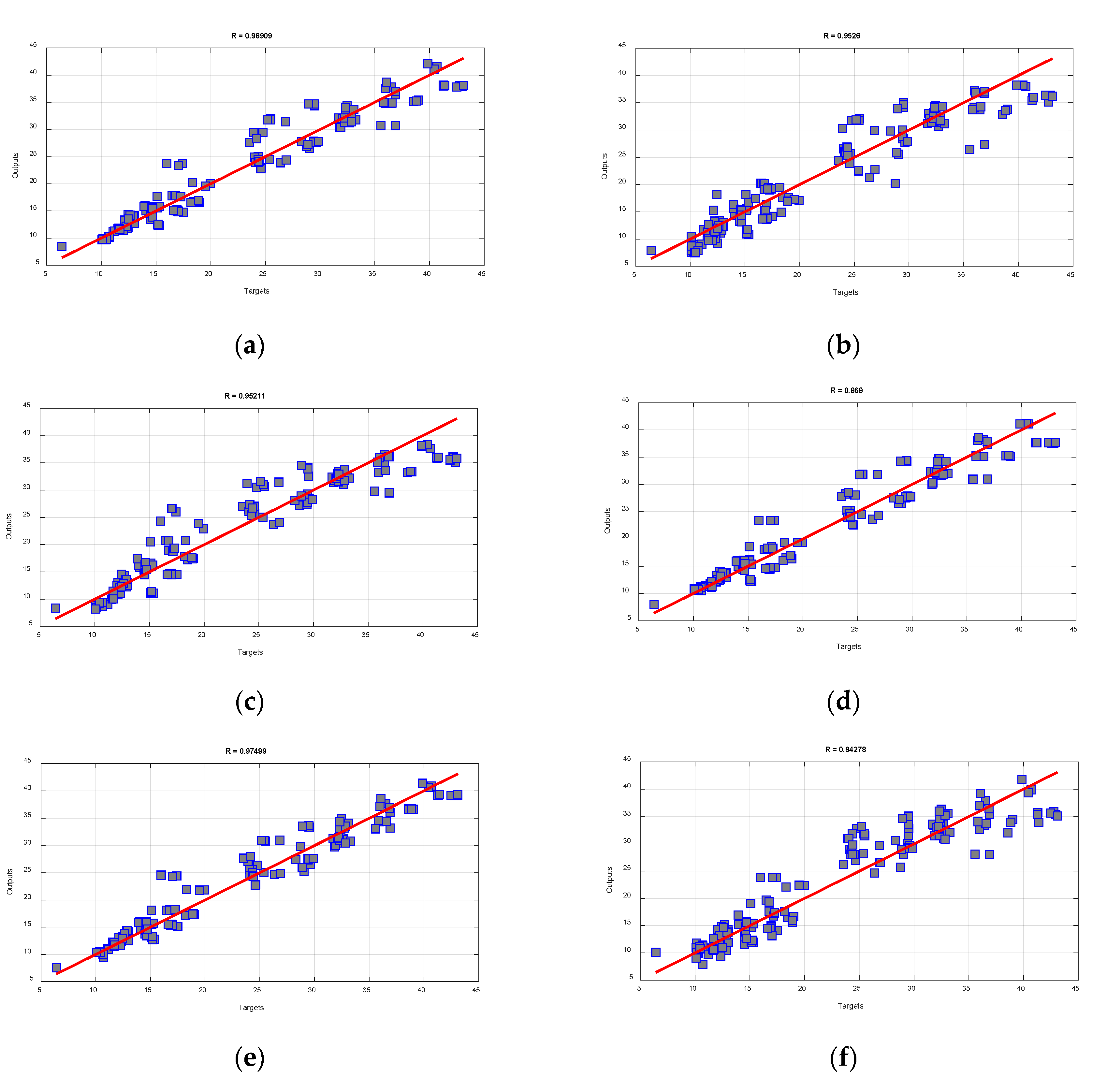
3.2. A Comparative Validation

The results in the previous section demonstrated the efficacy of the SOS–ANN in this study. This section provides a comparison between the SOS and six other algorithms, namely PO, HBO, HGSO, ASO, SFS, and CFOA that were similarly assigned to train the ANN. Their accuracy was compared to the SOS using the same criteria of RMSE, MAE, and R.

Table 3. Comparative assessment of the results (RMSE and MAE in kWh/m²).

Type	Model	Network Results
		Training			Testing
		MAE	RMSE	R	MAE	RMSE	R
Benchmark	PO–ANN	1.663	2.348	0.972	1.775	2.463	0.969
	HBO–ANN	2.301	3.084	0.953	2.395	3.119	0.952
	HGSO–ANN	2.152	2.912	0.957	2.234	3.054	0.952
	ASO–ANN	1.642	2.351	0.972	1.803	2.469	0.969
	SFS–ANN	1.493	2.002	0.980	1.648	2.222	0.974
	CFOA–ANN	2.377	3.148	0.950	2.559	3.358	0.942
	Vs.
Proposed	SOS–ANN	1.004	1.314	0.991	1.201	1.487	0.989

presents these gathered results.

According to the calculated RMSEs in the training phase, 2.348, 3.084, 2.912, 2.351, 2.002, and 3.148 for the PO–ANN, HBO–ANN, HGSO–ANN, ASO–ANN, SFS–ANN, and CFOA–ANN, respectively, the errors of all benchmark models are above the SOS–ANN. Similarly, this can also be said for the MAEs 1.663, 2.301, 2.152, 1.642, 1.493, and 2.377. The RMSE and MAE for the SOS–ANN were 1.004 and 1.314, respectively, which indicate a considerably better training performance.

Figure 5 depicts the correlation analysis executed for the training data. Comparing these graphs with Figure 3b, it can be observed that the SOS–ANN has produced more consistent results with target H_Ls (R-values of 0.991 vs. 0.972, 0.953, 0.957, 0.972, 0.980, and 0.950).

Similarly in the testing phase, the RMSE values were 2.463, 3.119, 3.054, 2.469, 2.222, and 3.358 along with the MAEs of 1.775, 2.395, 2.234, 1.803, 1.648, and 2.559, which were greater than those for the SOS–ANN (i.e., RMSE = 1.487 and MAE = 1.201). The smaller testing errors associated with the SOS algorithm indicate the higher potential of this algorithm for accurately predicting the H_L behavior.

Figure 6 shows the correlation results for the test data, displaying R-values of 0.969, 0.952, 0.952, 0.969, 0.974, and 0.942. More harmonious results for the SOS–ANN can be deduced regarding the R-value of 0.989 depicted in Figure 4b.

A deeper assessment of the values reported in Table 3 indicates a notable reduction in error magnitude when each of the benchmark algorithms is replaced with the SOS. For instance, in the training phase and terms of RMSE, the reductions range from 32.8% and 57.76% for SFS–ANN and CFOA–ANN, respectively. This range is 34.3% and 58.2%, respectively, for the MAE, and a 1.1% and 4.1% improvement, respectively, in the R-value.

As for the testing phase, the highest and lowest improvements can be reported again for the SFS–ANN and CFOA–ANN, respectively, with 27.12% and 53.06% reductions in RMSE. The corresponding values for MAE were 33.07% and 55.71%. Additionally, enhancements in the R index with SOS–ANN were in the range of 1.5% to 4.7%.

To achieve a more well-founded assessment, a relative error criterion called mean absolute percentage error (MAPE) was employed. The MAPE shows a percentage form of MAE (relative to the targets). Based on the obtained values, the SOS achieved training and testing results with 5.3 and 5.9% error, respectively, while the benchmarks attained MAPEs of 7.7, 11.5, 10.6, 7.4, 7.0, and 11.7 in the training phase and 7.9, 11.3, 10.7, 8.1, 7.4, and 11.8 in the testing phase. The SOS, therefore, enjoys lower error rates (below 6%).

3.3. Interpretation and Discussion

As is globally known, recent developments have provided reliable solutions to plenty of engineering challenges, especially in the energy sector. In the literature, much research can be found that focuses on estimating a specific parameter based on understanding how it is affected by influential parameters [62,63]. The models employed in this work followed the same policy to analyze the thermal behavior of buildings. The objective was fulfilled using sophisticated AI techniques and a dependable dataset from the literature.

In this section, the objective is to explain what the goodness of fit results means for each phase. First, regarding the training phase, some explanations were given in Section 2.1. The training data form around 80% of the whole dataset and were used for training the SOS–ANN. The word ‘training’ here means discovering the nonlinear relationship between the H_Ls and eight input parameters (i.e., C_R, S_A, S_W, S_R, H_T, O, S_G, and DS_G). Considering the training role that in this study was assigned to the SOS algorithm, this algorithm tried to find the best simultaneous contribution of input factors to the corresponding H_Ls by determining the weights and biases for the ANN. In so doing, the SOS analyzed 614 samples 1000 times to improve the solution. When the training results were quite promising, it meant that the SOS had great optimization potential. Altogether, the combination of SOS and ANN can understand the H_L behavior with high accuracy.

As for the testing phase, the knowledge learned by the SOS–ANN in the previous phase was applied to a new set of data to see how well it could predict the H_L for unseen situations. In other words, the results of this phase represented the generalizability of the model. Testing results were also quite promising with high accuracy. It can, therefore, be deduced that the SOS–ANN is reliable enough to predict the H_L by receiving new building characteristics.

From a methodological point of view, it is inferred that the weights and biases suggested by the SOS algorithm have created a powerful ANN. Back to Figure 2, the solution is considered a globally optimal response because metaheuristic algorithms take advantage of specific schemes to stay safe from computational drawbacks such as local minima and dimensional dangers [64,65].

Additionally, a comparison with several new metaheuristic techniques in Section 3.2 revealed that the solution of the SOS algorithm surpassed the PO, HBO, HGSO, ASO, SFS, and CFOA techniques. This betterment happened in both the training and testing phases reflecting the absolute superiority of the SOS. Therefore, this algorithm can capture a more realistic perception of the dependency of the H_L on building characteristics and can also yield a more reliable approximation for new building configurations. Moreover, having the same comparison among the benchmark algorithms, it is immediately apparent that the performance of the SFS algorithm was more promising than others; after that, the PO and ASO provided more reasonable results, while the performance of CFOA was the poorest.

Concerning the limitations of this study, there are some ideas for improving the generalizability of the models. Applying cross-validation with real-world buildings would further confirm their prediction competency in newer cases. Additionally, the models could be tested with additional energy datasets. Another potential idea is associating the cooling load with heating. In other words, developing a more comprehensive network that can predict the heating and cooling loads of a building simultaneously. However, developing a double-target ANN requires specific considerations (e.g., enlarging the output layer and relevant optimizable variables).

3.4. Literature Comparison

Besides the internal comparison performed for six algorithms within this study, the accuracy of the SOS was also assessed against several metaheuristic algorithms used in earlier studies for predicting the H_L.

Table 4. List of the metaheuristic algorithms used in earlier literature.

Study	Used Algorithm	Abbreviation	Developer
Tien Bui, et al. [36]	Genetic algorithm	GA	Holland [66]
	Imperialist competitive algorithm	ICA	Atashpaz-Gargari and Lucas [67]
Guo, et al. [45]	Wind-driven optimization	WDO	Bayraktar, et al. [68]
	Whale optimization algorithm	WOA	Mirjalili and Lewis [69]
	Spotted hyena optimization	SHO	Dhiman and Kumar [70]
	Salp swarm algorithm	SSA	Mirjalili, et al. [71]
Moayedi, et al. [72]	Grasshopper optimization algorithm	GOA	Saremi, et al. [73]
	Gray wolf optimization	GWO	Mirjalili, et al. [74]
Zhou, et al. [75]	Artificial bee colony	ABC	Karaboga [76]
	Particle swarm optimization	PSO	Kennedy and Eberhart [77]
Almutairi, et al. [42]	Firefly algorithm	FA	Yang [78]
	Optics-inspired optimization	OIO	Kashan [79]
	Shuffled complex evolution	SCE	Duan, et al. [80]
	Teaching–learning-based optimization	TLBO	Rao, et al. [81]

gives the details of the considered algorithms. They were then compared in Figure 7a,b in terms of the testing RMSE and MAE, respectively. Two positive notes regarding this comparison are that (i) all algorithms were in combination with an MLP neural network and (ii) the dataset exposed to all models was the same as the one used in this work (i.e., as developed by Tsanas and Xifara [48]). Thus, there are enough fair conditions that increase the reliability of this comparison.

From these figures, it was derived that there was a notable difference between the prediction error achieved in this study and that of previous studies. The MAE and RMSE of the SOS were 1.201 and 1.487, respectively, which are lower than all fourteen models. The SOS is most followed by the TLBO (MAE = 1.5804 and RMSE = 2.1103) and SCE (MAE = 1.6077 and RMSE = 2.2774) used by Almutairi, et al. [42]. Altogether, owing to the outperformance of SOS over (14 + 6 =) 20 similar rival algorithms, it can be said that the findings of this study have effectively improved the prediction of H_L.

4. Conclusions

The principal motivation for this work was to keep the concept of energy performance analysis updated with advances in metaheuristic science. A new metaheuristic algorithm called the symbiotic organism search algorithm was applied to an ANN network for analyzing and estimating the behavior of H_L in residential buildings. The findings revealed an excellent potential of the SOS algorithm in training an H_L-predictive ANN, owing to the provided weights and biases, as well as the favorable optimization path. A similarly great competency was observed for the results in the testing phase to prove the efficacy of this model in dealing with the unseen condition. Moreover, an extensive comparison with similar metaheuristic techniques (employed in both this study and the previous literature) was carried out, which showed that utilizing the SOS algorithm can potentially improve the accuracy of H_L simulation. To sum up, the proposed hybrid model is recommended for practical use such as optimizing energy components (e.g., HVAC systems) in energy-efficient buildings. However, implementing some ideas (e.g., creating a double-target network to support cooling load prediction simultaneously and the cross-validation of the models with multiple real-world data) is suggested to further increase the acceptability of the model in future studies.

References

1. Wolfram, C.; Shelef, O.; Gertler, P. How will energy demand develop in the developing world? J. Econ. Perspect. 2012, 26, 119–138. [Google Scholar] [CrossRef] [Green Version]
2. Keho, Y. What drives energy consumption in developing countries? The experience of selected African countries. Energy Policy 2016, 91, 233–246. [Google Scholar] [CrossRef]
3. Energy, G. CO2 Status Report; IEA (International Energy Agency): Paris, France, 2019. [Google Scholar]
4. Serghides, D.; Dimitriou, S.; Kyprianou, I. Mediterranean Hospital Energy Performance Mapping: The Energy Auditing as a Tool Towards Zero Energy Healthcare Facilities. In Sustainable Energy Development and Innovation; Springer: Berlin/Heidelberg, Germany, 2022; pp. 419–429. [Google Scholar]
5. Li, Y.; Kubicki, S.; Guerriero, A.; Rezgui, Y. Review of building energy performance certification schemes towards future improvement. Renew. Sustain. Energy Rev. 2019, 113, 109244. [Google Scholar] [CrossRef]
6. Li, X.; Liu, S.; Zhao, L.; Meng, X.; Fang, Y. An integrated building energy performance evaluation method: From parametric modeling to GA-NN based energy consumption prediction modeling. J. Build. Eng. 2022, 45, 103571. [Google Scholar] [CrossRef]
7. Ghadimi, M.; Ghadamian, H.; Hamidi, A.; Shakouri, M.; Ghahremanian, S. Numerical analysis and parametric study of the thermal behavior in multiple-skin façades. Energy Build. 2013, 67, 44–55. [Google Scholar] [CrossRef]
8. Ghadamian, H.; Ghadimi, M.; Shakouri, M.; Moghadasi, M.; Moghadasi, M. Analytical solution for energy modeling of double skin façades building. Energy Build. 2012, 50, 158–165. [Google Scholar] [CrossRef]
9. Shakouri, M.; Ghadamian, H. Energy Demand Analysis for Office Building Using Simulation Model and Statistical Method. Distrib. Gener. Altern. Energy J. 2022, 37, 1577–1612. [Google Scholar] [CrossRef]
10. Liu, X.; Tong, D.; Huang, J.; Zheng, W.; Kong, M.; Zhou, G. What matters in the e-commerce era? Modelling and mapping shop rents in Guangzhou, China. Land Use Policy 2022, 123, 106430. [Google Scholar] [CrossRef]
11. Han, Y.; Yan, X.; Piroozfar, P. An overall review of research on prefabricated construction supply chain management. Eng. Constr. Archit. Manag. 2022; ahead-of-print. [Google Scholar] [CrossRef]
12. Han, Y.; Xu, X.; Zhao, Y.; Wang, X.; Chen, Z.; Liu, J. Impact of consumer preference on the decision-making of prefabricated building developers. J. Civ. Eng. Manag. 2022, 28, 166–176. [Google Scholar] [CrossRef]
13. Gu, M.; Cai, X.; Fu, Q.; Li, H.; Wang, X.; Mao, B. Numerical Analysis of Passive Piles under Surcharge Load in Extensively Deep Soft Soil. Buildings 2022, 12, 1988. [Google Scholar] [CrossRef]
14. Kordestani, H.; Zhang, C.; Masri, S.F.; Shadabfar, M. An empirical time-domain trend line-based bridge signal decomposing algorithm using Savitzky–Golay filter. Struct. Control Health Monit. 2021, 28, e2750. [Google Scholar] [CrossRef]
15. Fu, Q.; Gu, M.; Yuan, J.; Lin, Y. Experimental study on vibration velocity of piled raft supported embankment and foundation for ballastless high speed railway. Buildings 2022, 12, 1982. [Google Scholar] [CrossRef]
16. Li, S. Efficient algorithms for scheduling equal-length jobs with processing set restrictions on uniform parallel batch machines. Math. Bios. Eng 2022, 19, 10731–10740. [Google Scholar] [CrossRef]
17. Lu, S.; Guo, J.; Liu, S.; Yang, B.; Liu, M.; Yin, L.; Zheng, W. An improved algorithm of drift compensation for olfactory sensors. Appl. Sci. 2022, 12, 9529. [Google Scholar] [CrossRef]
18. Zhang, Z.; Li, W.; Yang, J. Analysis of stochastic process to model safety risk in construction industry. J. Civ. Eng. Manag. 2021, 27, 87–99. [Google Scholar] [CrossRef]
19. Liu, L.; Li, Z.; Fu, X.; Liu, X.; Li, Z.; Zheng, W. Impact of Power on Uneven Development: Evaluating Built-Up Area Changes in Chengdu Based on NPP-VIIRS Images (2015–2019). Land 2022, 11, 489. [Google Scholar] [CrossRef]
20. Chen, J.; Tong, H.; Yuan, J.; Fang, Y.; Gu, R. Permeability prediction model modified on kozeny-carman for building foundation of clay soil. Buildings 2022, 12, 1798. [Google Scholar] [CrossRef]
21. Zhan, C.; Dai, Z.; Soltanian, M.R.; de Barros, F.P. Data-Worth Analysis for Heterogeneous Subsurface Structure Identification With a Stochastic Deep Learning Framework. Water Resour. Res. 2022, 58, e2022WR033241. [Google Scholar] [CrossRef]
22. Dang, W.; Guo, J.; Liu, M.; Liu, S.; Yang, B.; Yin, L.; Zheng, W. A semi-supervised extreme learning machine algorithm based on the new weighted kernel for machine smell. Appl. Sci. 2022, 12, 9213. [Google Scholar] [CrossRef]
23. Zhang, K.; Wang, Z.; Chen, G.; Zhang, L.; Yang, Y.; Yao, C.; Wang, J.; Yao, J. Training effective deep reinforcement learning agents for real-time life-cycle production optimization. J. Pet. Sci. Eng. 2022, 208, 109766. [Google Scholar] [CrossRef]
24. Fumo, N. A review on the basics of building energy estimation. Renew. Sustain. Energy Rev. 2014, 31, 53–60. [Google Scholar] [CrossRef]
25. Sharif, S.A.; Hammad, A. Developing surrogate ANN for selecting near-optimal building energy renovation methods considering energy consumption, LCC and LCA. J. Build. Eng. 2019, 25, 100790. [Google Scholar] [CrossRef]
26. Seo, J.; Kim, S.; Lee, S.; Jeong, H.; Kim, T.; Kim, J. Data-driven approach to predicting the energy performance of residential buildings using minimal input data. Build. Environ. 2022, 214, 108911. [Google Scholar] [CrossRef]
27. Seyedzadeh, S.; Rahimian, F.P.; Glesk, I.; Roper, M. Machine learning for estimation of building energy consumption and performance: A review. Vis. Eng. 2018, 6, 1–20. [Google Scholar] [CrossRef]
28. Shao, M.; Wang, X.; Bu, Z.; Chen, X.; Wang, Y. Prediction of energy consumption in hotel buildings via support vector machines. Sustain. Cities Soc. 2020, 57, 102128. [Google Scholar] [CrossRef]
29. Kardani, N.; Bardhan, A.; Kim, D.; Samui, P.; Zhou, A. Modelling the energy performance of residential buildings using advanced computational frameworks based on RVM, GMDH, ANFIS-BBO and ANFIS-IPSO. J. Build. Eng. 2021, 35, 102105. [Google Scholar] [CrossRef]
30. Adedeji, P.A.; Akinlabi, S.; Madushele, N.; Olatunji, O.O. Hybrid adaptive neuro-fuzzy inference system (ANFIS) for a multi-campus university energy consumption forecast. Int. J. Ambient Energy 2022, 43, 1685–1694. [Google Scholar] [CrossRef]
31. Ngo, N.-T.; Pham, A.-D.; Truong, T.T.H.; Truong, N.-S.; Huynh, N.-T.; Pham, T.M. An ensemble machine learning model for enhancing the prediction accuracy of energy consumption in buildings. Arab. J. Sci. Eng. 2022, 47, 4105–4117. [Google Scholar] [CrossRef]
32. Elias, R.; Issa, R.R. Artificial-Neural-Network-Based Model for Predicting Heating and Cooling Loads on Residential Buildings. In Computing in Civil Engineering; ASCE: Reston, VA, USA, 2021; pp. 140–147. [Google Scholar]
33. Jang, J.; Han, J.; Leigh, S.-B. Prediction of heating energy consumption with operation pattern variables for non-residential buildings using LSTM networks. Energy Build. 2022, 255, 111647. [Google Scholar] [CrossRef]
34. Zhou, Y.; Wang, L.; Qian, J. Application of Combined Models Based on Empirical Mode Decomposition, Deep Learning, and Autoregressive Integrated Moving Average Model for Short-Term Heating Load Predictions. Sustainability 2022, 14, 7349. [Google Scholar] [CrossRef]
35. Koschwitz, D.; Frisch, J.; Van Treeck, C. Data-driven heating and cooling load predictions for non-residential buildings based on support vector machine regression and NARX Recurrent Neural Network: A comparative study on district scale. Energy 2018, 165, 134–142. [Google Scholar] [CrossRef]
36. Tien Bui, D.; Moayedi, H.; Anastasios, D.; Kok Foong, L. Predicting heating and cooling loads in energy-efficient buildings using two hybrid intelligent models. Appl. Sci. 2019, 9, 3543. [Google Scholar] [CrossRef] [Green Version]
37. Hu, J.; Zheng, W.; Zhang, S.; Li, H.; Liu, Z.; Zhang, G.; Yang, X. Thermal load prediction and operation optimization of office building with a zone-level artificial neural network and rule-based control. Appl. Energy 2021, 300, 117429. [Google Scholar] [CrossRef]
38. Shah, P.; Sekhar, R.; Kulkarni, A.J.; Siarry, P. Metaheuristic Algorithms in Industry 4.0; CRC Press: Boca Raton, FL, USA, 2021. [Google Scholar]
39. Moayedi, H.; Mehrabi, M.; Mosallanezhad, M.; Rashid, A.S.A.; Pradhan, B. Modification of landslide susceptibility mapping using optimized PSO-ANN technique. Eng. Comput. 2019, 35, 967–984. [Google Scholar] [CrossRef]
40. Asadi Nalivan, O.; Mousavi Tayebi, S.A.; Mehrabi, M.; Ghasemieh, H.; Scaioni, M. A hybrid intelligent model for spatial analysis of groundwater potential around Urmia Lake, Iran. Stoch. Environ. Res. Risk Assess. 2022, 1–18. [Google Scholar] [CrossRef]
41. Pachauri, N.; Ahn, C.W. In Regression Tree Ensemble Learning-Based Prediction of the Heating and Cooling Loads of Residential Buildings; Building Simulation 2022; Springer: Berlin/Heidelberg, Germany, 2022; pp. 1–15. [Google Scholar]
42. Almutairi, K.; Algarni, S.; Alqahtani, T.; Moayedi, H.; Mosavi, A. A TLBO-Tuned Neural Processor for Predicting Heating Load in Residential Buildings. Sustainability 2022, 14, 5924. [Google Scholar] [CrossRef]
43. Xu, Y.; Li, F.; Asgari, A. Prediction and optimization of heating and cooling loads in a residential building based on multi-layer perceptron neural network and different optimization algorithms. Energy 2022, 240, 122692. [Google Scholar] [CrossRef]
44. Moayedi, H.; Mosavi, A. Synthesizing multi-layer perceptron network with ant lion biogeography-based dragonfly algorithm evolutionary strategy invasive weed and league champion optimization hybrid algorithms in predicting heating load in residential buildings. Sustainability 2021, 13, 3198. [Google Scholar] [CrossRef]
45. Guo, Z.; Moayedi, H.; Foong, L.K.; Bahiraei, M. Optimal modification of heating, ventilation, and air conditioning system performances in residential buildings using the integration of metaheuristic optimization and neural computing. Energy Build. 2020, 214, 109866. [Google Scholar] [CrossRef]
46. Wu, H.; Zhou, Y.; Luo, Q.; Basset, M.A. Training feedforward neural networks using symbiotic organisms search algorithm. Comput. Intell. Neurosci. 2016, 2016, 9063065. [Google Scholar] [CrossRef] [PubMed] [Green Version]
47. Miao, F.; Yao, L.; Zhao, X. Evolving convolutional neural networks by symbiotic organisms search algorithm for image classification. Appl. Soft Comput. 2021, 109, 107537. [Google Scholar] [CrossRef]
48. Tsanas, A.; Xifara, A. Accurate quantitative estimation of energy performance of residential buildings using statistical machine learning tools. Energy Build. 2012, 49, 560–567. [Google Scholar] [CrossRef]
49. Pessenlehner, W.; Mahdavi, A. Building Morphology, Transparence, and Energy Performance; AIVC: Sint-Stevens-Woluwe, Belgium, 2003. [Google Scholar]
50. Huang, Y.; Niu, J.-L.; Chung, T.-M. Comprehensive analysis on thermal and daylighting performance of glazing and shading designs on office building envelope in cooling-dominant climates. Appl. Energy 2014, 134, 215–228. [Google Scholar] [CrossRef]
51. Papadopoulos, S.; Azar, E.; Woon, W.-L.; Kontokosta, C.E. Evaluation of tree-based ensemble learning algorithms for building energy performance estimation. J. Build. Perform. Simul. 2018, 11, 322–332. [Google Scholar] [CrossRef]
52. Moayedi, H.; Mosavi, A. Suggesting a stochastic fractal search paradigm in combination with artificial neural network for early prediction of cooling load in residential buildings. Energies 2021, 14, 1649. [Google Scholar] [CrossRef]
53. Zheng, S.; Lyu, Z.; Foong, L.K. Early prediction of cooling load in energy-efficient buildings through novel optimizer of shuffled complex evolution. Eng. Comput. 2020, 38, 105–119. [Google Scholar] [CrossRef]
54. Wu, D.; Foong, L.K.; Lyu, Z. Two neural-metaheuristic techniques based on vortex search and backtracking search algorithms for predicting the heating load of residential buildings. Eng. Comput. 2020, 38, 647–660. [Google Scholar] [CrossRef]
55. Cheng, M.-Y.; Prayogo, D. Symbiotic organisms search: A new metaheuristic optimization algorithm. Comput. Struct. 2014, 139, 98–112. [Google Scholar] [CrossRef]
56. Zhou, Y.; Wu, H.; Luo, Q.; Abdel-Baset, M. Automatic data clustering using nature-inspired symbiotic organism search algorithm. Knowl.-Based Syst. 2019, 163, 546–557. [Google Scholar] [CrossRef]
57. Abdullahi, M.; Ngadi, M.A. Symbiotic organism search optimization based task scheduling in cloud computing environment. Future Gener. Comput. Syst. 2016, 56, 640–650. [Google Scholar] [CrossRef]
58. Mehrabi, M.; Pradhan, B.; Moayedi, H.; Alamri, A. Optimizing an adaptive neuro-fuzzy inference system for spatial prediction of landslide susceptibility using four state-of-the-art metaheuristic techniques. Sensors 2020, 20, 1723. [Google Scholar] [CrossRef] [PubMed] [Green Version]
59. Zhao, Y.; Hu, H.; Song, C.; Wang, Z. Predicting compressive strength of manufactured-sand concrete using conventional and metaheuristic-tuned artificial neural network. Measurement 2022, 194, 110993. [Google Scholar] [CrossRef]
60. Mehrabi, M.; Moayedi, H. Landslide susceptibility mapping using artificial neural network tuned by metaheuristic algorithms. Environ. Earth Sci. 2021, 80, 1–20. [Google Scholar] [CrossRef]
61. Mehrabi, M. Landslide susceptibility zonation using statistical and machine learning approaches in Northern Lecco, Italy. Nat. Hazards 2021, 111, 901–937. [Google Scholar] [CrossRef]
62. Liao, L.; Du, L.; Guo, Y. Semi-supervised SAR target detection based on an improved faster R-CNN. Remote Sens. 2021, 14, 143. [Google Scholar] [CrossRef]
63. Amasyali, K.; El-Gohary, N. Machine learning for occupant-behavior-sensitive cooling energy consumption prediction in office buildings. Renew. Sustain. Energy Rev. 2021, 142, 110714. [Google Scholar] [CrossRef]
64. Moayedi, H.; Mehrabi, M.; Bui, D.T.; Pradhan, B.; Foong, L.K. Fuzzy-metaheuristic ensembles for spatial assessment of forest fire susceptibility. J Environ. Manag. 2020, 260, 109867. [Google Scholar] [CrossRef]
65. Nguyen, H.; Mehrabi, M.; Kalantar, B.; Moayedi, H.; Abdullahi, M.a.M. Potential of hybrid evolutionary approaches for assessment of geo-hazard landslide susceptibility mapping. Geomat. Nat. Hazards Risk 2019, 10, 1667–1693. [Google Scholar] [CrossRef] [Green Version]
66. Holland, J.H. Genetic algorithms. Sci. Am. 1992, 267, 66–73. [Google Scholar] [CrossRef]
67. Atashpaz-Gargari, E.; Lucas, C. Imperialist competitive algorithm: An algorithm for optimization inspired by imperialistic competition. In Proceedings of the 2007 IEEE Congress on Evolutionary Computation, Singapore, 25–28 September 2007; IEEE: New York, NY, USA, 2007; pp. 4661–4667. [Google Scholar]
68. Bayraktar, Z.; Komurcu, M.; Werner, D.H. Wind Driven Optimization (WDO): A novel nature-inspired optimization algorithm and its application to electromagnetics. In Proceedings of the 2010 IEEE Antennas and Propagation Society International Symposium, Toronto, ON, Canada, 11–17 July 2010; IEEE: New York, NY, USA, 2010; pp. 1–4. [Google Scholar]
69. Mirjalili, S.; Lewis, A. The whale optimization algorithm. Adv. Eng. Softw. 2016, 95, 51–67. [Google Scholar] [CrossRef]
70. Dhiman, G.; Kumar, V. Multi-objective spotted hyena optimizer: A Multi-objective optimization algorithm for engineering problems. Knowl.-Based Syst. 2018, 150, 175–197. [Google Scholar] [CrossRef]
71. Mirjalili, S.; Gandomi, A.H.; Mirjalili, S.Z.; Saremi, S.; Faris, H.; Mirjalili, S.M. Salp Swarm Algorithm: A bio-inspired optimizer for engineering design problems. Adv. Eng. Softw. 2017, 114, 163–191. [Google Scholar] [CrossRef]
72. Moayedi, H.; Nguyen, H.; Foong, L. Nonlinear evolutionary swarm intelligence of grasshopper optimization algorithm and gray wolf optimization for weight adjustment of neural network. Eng. Comput. 2019, 37, 1265–1275. [Google Scholar] [CrossRef]
73. Saremi, S.; Mirjalili, S.; Lewis, A. Grasshopper optimisation algorithm: Theory and application. Adv. Eng. Softw. 2017, 105, 30–47. [Google Scholar] [CrossRef] [Green Version]
74. Mirjalili, S.; Mirjalili, S.M.; Lewis, A. Grey wolf optimizer. Adv. Eng. Softw. 2014, 69, 46–61. [Google Scholar] [CrossRef] [Green Version]
75. Zhou, G.; Moayedi, H.; Bahiraei, M.; Lyu, Z. Employing artificial bee colony and particle swarm techniques for optimizing a neural network in prediction of heating and cooling loads of residential buildings. J. Clean. Prod. 2020, 254, 120082. [Google Scholar] [CrossRef]
76. Karaboga, D. An Idea Based on Honey Bee Swarm for Numerical Optimization; Technical Report-tr06; Erciyes University, Engineering Faculty, Computer Engineering Department: Kayseri, Turkey, 2005. [Google Scholar]
77. Kennedy, J.; Eberhart, R. Particle swarm optimization. In Proceedings of the ICNN′95—International Conference on Neural Networks, Perth, Australia, 27 November–1 December 1995; Volume 4, pp. 1942–1948. [Google Scholar]
78. Yang, X.-S. Firefly algorithm. Nat.-Inspired Metaheuristic Algorithms 2008, 20, 79–90. [Google Scholar]
79. Kashan, A.H. A new metaheuristic for optimization: Optics inspired optimization (OIO). Comput. Oper. Res. 2015, 55, 99–125. [Google Scholar] [CrossRef]
80. Duan, Q.; Gupta, V.K.; Sorooshian, S. Shuffled complex evolution approach for effective and efficient global minimization. J. Optim. Theory Appl. 1993, 76, 501–521. [Google Scholar] [CrossRef]
81. Rao, R.V.; Savsani, V.J.; Vakharia, D. Teaching–learning-based optimization: A novel method for constrained mechanical design optimization problems. Comput.-Aided Des. 2011, 43, 303–315. [Google Scholar] [CrossRef]
Figure 1. Scatter and histogram charts of the dataset factors.
Buildings 13 00727 g001
Figure 2. SOS optimization curve.
Buildings 13 00727 g002
Figure 3. The quality of the SOS–ANN results in terms of error (a) and correlation (b) for the training phase (HL in kWh/m2).
Buildings 13 00727 g003
Figure 4. The quality of the SOS–ANN results in terms of error (a) and correlation (b) for the testing phase (HL in kWh/m2).
Buildings 13 00727 g004
Figure 5. The correlations between the target HLs and training results for (a) PO–ANN, (b) HBO–ANN, (c) HGSO–ANN, (d) ASO–ANN, (e) SFS–ANN, and (f) CFOA–ANN (all values in kWh/m2).
Buildings 13 00727 g005aBuildings 13 00727 g005b
Figure 6. The correlations between the target HLs and test results for (a) PO–ANN, (b) HBO–ANN, (c) HGSO–ANN, (d) ASO–ANN, (e) SFS–ANN, and (f) CFOA–ANN (all values in kWh/m2).
Buildings 13 00727 g006
Figure 7. Column charts comparing the SOS with previous models in terms of (a) RMSE and (b) MAE, both in kWh/m2.
Buildings 13 00727 g007