Time-Domain Structural Damage and Loss Estimates for Wind Loads: Road to Resilience-Targeted and Smart Buildings Design

Abstract

A time-domain wind-induced damage evaluation for the risk- and resilience-targeted design of building structures requires nonlinear dynamic analysis (NDA) solvers to handle long duration input loads. Moreover, post-construction damage identification based on real-time vibration monitoring depends on accurate damage simulation from the design stage and available artificial intelligence (AI)-based technology. In this paper, an integrated time-domain approach for the performance-based analysis and design for wind is presented. The nonlinear dynamic analysis (NDA) is performed with the Force Analogy Method (FAM) and the state–space formulation to solve the nonlinear equations of motion. Then, the Incremental Dynamic Analysis (IDA) is used to perform probabilistic fragility analyses for a typical reinforced concrete (RC) frame structure. The analysis also provides estimates of expected losses, gives the building owners business support data to compare, e.g., the final annual building income (FABI), the cost of repair and the function recovery duration for various wind events in an integrated resilience-based building design framework. This provides the basis for mapping structural damage on large urban scales and for straightforward quantification of wind-induced damage from available response acceleration time-series acquired from real-time vibration monitoring.

1. Introduction

The United Nations Office for Disasters Risk Reduction-UNISDR reported a total of 2049 disasters caused by extreme wind events from 1998 to 2017 (report available at https://www.undrr.org/, accessed on 5 June 2022). This number accounts for approximately 30% of the total number of natural disasters. According to the same report, the disasters affected 726 million people (16% of the total world population), and the associated economic losses were valued at USD 1330 billion (46% of the total amount of disaster-generated economic losses). For instance, the total economic losses after the hurricanes Katrina, Rita, and Wilma (2005) were USD 201 billion, and another USD 245 billion in losses were generated by hurricanes Harvey, Irma and Maria (2017).

Consequently, society needs the civil engineering community to develop standardized, higher-level integrated analysis and design frameworks to quantify the structural damage and reduce the risk induced by extreme wind events, such as thunderstorms or downbursts. Once extreme wind events are accurately reproduced through reliable models (e.g., THUNDERR project https://cordis.europa.eu/project/id/741273, accessed on 5 June 2022) and accurate wind tunnel measurements, structural engineers, technology specialists and project managers will be able to quantify wind-induced damage, structural and non-structural associated economic losses, function recovery durations and associated costs. The extension of current structural design tools to a more accurate and refined end-product level will create the capability to develop a full resilience-targeted structural design in the future. This higher-level integrated approach requires efficient nonlinear dynamic analysis solvers to handle the aerodynamic input wind loads and linked analysis modules.

The Equivalent Static Wind Loads (ESWLs) approach is currently used in the structural design. This approach provides aerodynamic wind load distribution to practitioners with a limited degree of accuracy for typical building shapes up to 200 m high. For taller buildings, however, many national codes, such as the Romanian Wind Design Code CR1-1-4/2012 (EC1 format), suggest the use of experimental investigation techniques like the wind tunnel testing [1].

In the last two decades, studies conducted on tall generic buildings using on one hand, national code practices from various countries, and on the other hand, a database-enabled procedure provided by, e.g., the NatHaz Aerodynamic Loads Database (NALD) [2,3], revealed a large variability of structural response parameters. This is reported to be attributable to the mean wind speed profile definition, wind speed averaging duration, turbulence intensity profile and the pressure/force coefficients distribution [4].

Automated structural analysis and design based on a myriad of national code requirements is usually performed using commercial structural analysis software. However, despite more affordable access to experimental facilities or Computational Fluid Dynamics (CFD)-based tools, none of the commercial computational platforms is tailored to incorporate simultaneous pressure measurements for a time-domain based analysis and design fluent framework. Moreover, the actual step-by-step numerical integration solvers usually fail to handle nonlinear structural models subjected to long duration input loads.

The concept of database-assisted design (DAD) was initially developed by Whalen et al. (2000) for low-rise buildings subjected to time-series of loads obtained from wind pressure measurements [5]. Comprehensive development work performed at the National Institute of Standards and Technology (NIST) later extended DAD to tall, flexible buildings. The computational package developed at NIST performs dynamic response analysis for tall, flexible, linear-elastic behavior structures subjected to simultaneous pressure time-histories from wind tunnel measurements. Time-history response and peak response values are obtained using the modal approach and predefined influence coefficients of the internal forces of structural members. Thus, the preliminary design check is straightforward and performed in the time-domain using the demand-to-capacity ratios approach [6,7,8,9,10,11].

Later, Kwon et al. (2008) [12] and Kareem and Kwon (2017) [13] suggested using virtual tools for the computation of wind-induced effects on structures.

A convergent work towards computation automation based on the DAD approach was performed at the Technical University of Civil Engineering Bucharest (UTCB). The time-domain computational framework developed by the Structural Dynamics Group consists of linked modules, including climatological data, aerodynamic data, modeling and structural analysis and a check of the preliminary design of structural members [14].

Implementation of a resilience-targeted design consisting of fragility assessment, damage evaluation, loss estimates, and function recovery duration modules based on an efficient nonlinear solver and large hardware capabilities for 2D and 3D models are presented in Nica et al. (2022) [15], Iancovici et al. (2022) [16] and Iancovici et al. (2022) [17].

This paper first discusses the current practice for obtaining wind aerodynamic loads for structural analysis and design. Testing time-histories of wind loads are obtained by using the NOWS (NatHaz on-line wind simulator) [3]. Extensive signal processing is performed to extract the basic parameters of wind loads that will later relate with the extent of structural damage.

Second, the basic features of nonlinear dynamic analysis (NDA) based on the Force Analogy Method (FAM) approach to solve the nonlinear equations of motion for 2D structural models subjected to long duration time-histories of wind loads are presented. Thus, the FAM is incorporated in a ©Matlab and Simulink-based analysis package [18] able to handle multiple long duration time-histories of testing wind loads. The time-history response parameters are straightforwardly used as the prerequisite for the next, higher level analysis modules of damage evaluation, probabilistic fragility, and loss estimation.

Third, a large number of nonlinear dynamic analyses (NDAs) are performed on a typical reinforced concrete (RC) frame structure in order to monitor and quantify the extent of damage at each section, element, story and structural level using the damage index definition proposed by Park and Ang (1985) [19].

Last, by using the Incremental Dynamic Analysis (IDA) approach [20] for wind loads and the Multiple Stripe Method (Jalayer and Cornell, 2009) [21], the structural fragility and loss estimates in a full probabilistic framework are obtained.

Following the provisions of the Prestandard for Performance-Based Wind Design (2019) [22], a unified Performance-Based Design (PBD) framework for both seismic- and wind-loads appear to be applicable in the not-too-distant future.

2. Aerodynamic Wind Loads for Structural Analysis

The ESWLs in Romanian wind design [1] are computed from the design base (reference) wind pressure averaged on a 10 min duration at a 10 m reference height above ground level. This corresponds to 2% probability of yearly exceedance, i.e., 50 years mean return interval (MRI).

The High Frequency Force Balance (HFFB) technique or the wind tunnel test (WT) are recommended experimental techniques for more accurate wind-induced pressure distribution estimates on buildings taller than 200 m and particular shapes [11].

Additionally, the Computational Fluid Dynamics (CFD)-based pressure evaluation tool is a candidate for accurate estimates, especially for applications in large-scale urban environments.

For the purposes of this study, ten low-correlated wind events were considered for analyses. Fluctuating wind speed testing time-histories were generated over one-hour duration by using the NatHaz on-line wind simulator (NOWS) for exposure category C-type terrain as defined by the ASCE 7-10 code [23], using a discrete frequency function based on Cholesky decomposition and a Fast Fourier Transform (FFT) scheme (available reference http://windsim.ce.nd.edu/gew_init2.html, accessed on 10 May 2019). The fluctuating wind speed testing time-histories for elevations up to 40 m are associated with reference mean wind speeds ranging from 5 m/s to 50 m/s, at 10 m above ground level, averaged on 3 s.

Typical fluctuating wind speed time-histories and the corresponding power spectral density (PSD) function are shown in Figure 1.

The turbulence intensity (I) and the gust factor (GF) distribution for all generated wind speed time-series are given in Figure 2.

In the current structural design practice based on recorded time-series of wind loads, the frequency content and the energy-based indicator of velocity pressure [24] are important parameters to be extracted and related to structurally induced damage.

Thus, the time-instant energy of the fluctuating wind speed component $u\left(z,t\right)$ at a given elevation $z$ above ground level is given by

$$E_u\left(z,t\right)=\underset{0}{\overset{t}{{\displaystyle \int }}}{u}^2\left(z,t\right)dt$$

(1)

The mean wind speed profiles corresponding to the ten wind events and the fluctuating wind speed energy ratios are represented in Figure 3. Thus, a 50 m/s reference mean wind speed event corresponding fluctuating component will generate roughly 80 times larger total energy than the total energy corresponding to a 5 m/s reference mean wind speed event.

The fluctuating wind speed component frequency bandwidth indicator is given by the following relationship [24]

$$\epsilon =\sqrt{1-\frac{{\lambda }_2^2}{{\lambda }_0{\lambda }_4}}\in \left(0,1\right)$$

(2)

The spectral moment of the ith order about the mean in Equation (2) is given by

$${\lambda }_i=\underset{0}{\overset{{\omega }_N}{{\displaystyle \int }}}{\omega }^i{S}_u\left(\omega \right)d\omega$$

(3)

where $S_u\left(\omega \right)$ represents the power spectral density (PSD) of the fluctuating wind speed component, and ${\omega }_N$ is the Nyquist circular frequency [24].

The distribution of fluctuating wind speed frequency bandwidth indicator over the height for all ten wind events is presented in Figure 4.

The frequency bandwidth decreases with the elevation and provides larger values for higher reference mean wind speeds.

The time-history of wind pressure at elevation z above the ground, namely $p\left(z,t\right)$, is defined as

$$p\left(z,t\right)= \frac{1}{2}{\rho }_{air}{C}_p{\left[\overline{u}\left(z\right)+u\left(z,t\right)\right]}^2$$

(4)

where ${\rho }_{air}=1.23 \mathrm{kg}/{\mathrm{m}}^3$ is the air density, $\overline{u}\left(z\right)$ is the mean wind speed at elevation z above the ground, and $u\left(z,t\right)$ is the fluctuating wind speed component at the same elevation z. $C_p$ is the mean pressure coefficient at a specified location on the building’s façade. In this paper, $C_p$ is taken as 0.8 for the windward and −0.7 for the leeward.

The aerodynamic wind force is therefore given by

$$F\left(z,t\right)=p\left(z,t\right)·A\left(z\right)$$

(5)

where $A\left(z\right)$ is the tributary area of the building façade considered at elevation z above the ground.

Net aerodynamic testing wind forces are straightforwardly used for the nonlinear dynamic analysis and subsequent damage evaluation, probabilistic fragility and loss estimates associated with various wind events.

3. Inelastic Response Analysis by the Force Analogy Method (FAM) and State–Space Formulation

The wind-induced structural response of an MDOF system results from solving the second order differential equations of motion, i.e.,

$$\mathit{M}\ddot{\mathit{x}}\left(\mathit{t}\right)+\mathit{C}\dot{\mathit{x}}\left(\mathit{t}\right)+{\mathit{F}}_{\mathit{r}}\left(\mathit{x},\dot{\mathit{x}},\mathit{t}\right)=\mathit{F}\left(\mathit{t}\right)$$

(6)

where $\mathit{M}$ and $\mathit{C}$ are the mass and damping matrices, $\ddot{\mathit{x}}\left(\mathit{t}\right),\dot{\mathit{x}} \left(\mathit{t}\right) \mathrm{and} \mathit{x} \left(\mathit{t}\right)$ are the response acceleration, velocity, and displacement vectors, and $\mathit{F}\left(\mathit{t}\right)$ aggregates the time-histories of aerodynamic wind loads, typically consisting of along-, across- and torque-induced load components.

The nonlinear effects induced by physical (inelastic behavior), geometrical or various interaction phenomena (e.g., soil-structure, fluid-structure, or internal energy dissipation for unconventional structures) might significantly influence the structural behavior. The restoring forces vector ${\mathit{F}}_{\mathit{r}}$ reproduces the effects of linear-elastic or nonlinear behavior (i.e., physical or/and geometrical) so that Equation (6) can be rewritten as

$$\mathit{M}\ddot{\mathit{x}}\left(\mathit{t}\right)+\mathit{C}\dot{\mathit{x}}\left(\mathit{t}\right)+\mathit{K}\left(\mathit{x}\right)\mathit{x}\left(\mathit{t}\right)=\mathit{F}\left(\mathit{t}\right)$$

(7)

where the stiffness is a function of response displacement. For linear-elastic systems, $\mathit{K}$ is the initial elastic stiffness matrix of the structure.

The physical nonlinearity of members can be modeled with discrete plasticity or distributed plasticity. A vast literature describes the results of extensive investigations performed to accurately reproduce the nonlinear behavior and to accommodate the analysis models and methods with available computational resources [25,26].

For typical building structures, the discrete plasticity plastic hinge model (PH) is largely used and assigned to the potential plastic zones of members. The sectional hysteretic rules adopted aim to primarily reproduce the stiffness and strength deterioration under cyclic loading.

The fiber model (FM) seems to be the most effective distributed plasticity model [27] when compared to the finite length plastic hinge model (FLPH), a reasonable computational compromise between PH and FM models [28].

The two methods currently used to compute the dynamic response are (i) the Mode Superposition Method, numerically efficient but restricted to linear-elastic behavior structures, and (ii) the Direct Integration Method, with the largest applicability but numerically inefficient mostly due to the stiffness matrix required update at each integration time-step.

The Force Analogy Method (FAM) for the integration of nonlinear equations of motion was first proposed by Lin (1968) [29]. The continuous development for seismic applications made by Hart and Wong (1999), Zhao and Wong (2006), Wang and Wong (2007), Zhang et al. (2007), Li and Wong (2014) and Li et al. (2015) [30,31,32,33,34,35] refined the method to include physical and geometric nonlinearity effects for reinforced concrete and steel frame structures.

Later, the FAM-based nonlinear dynamic analysis was successfully applied for time-series of wind loads [36] and to predict the pounding-induced seismic inelastic behavior of RC structures [37].

For the sake of clarity, the concept of the Force Analogy Method (FAM) is first illustrated using the Single Degree of Freedom system (SDOF) and then extended to Multiple Degree of Freedom systems (MDOF) to model the current building structures [29,30,34].

3.1. Force Analogy Method (FAM) Approach for SDOF Systems

The equation of motion of an inelastic SDOF system (Figure 5), defined by mass coefficient- m, damping coefficient- c and restoring force characteristics- $F_r,$ subjected to an arbitrary load $F\left(t\right)$ is given by

$$m\ddot{x}+c\dot{x}+F_r\left(x,\dot{x},t\right)=F\left(t\right)$$

(8)

The plastic hinge (PH) is attributed to the potential plastic zone. From the force–displacement relationship (Figure 5), the restoring force at response displacement $x$ is

$$F_r=F_y+F_{ri}=k{x}_y+k_{py}(x-x_y)$$

(9)

where $x$ is the total response displacement, $F_y$ and $x_y$ are the restoring force and the corresponding displacement at yield point, $k$ is the initial (elastic) stiffness, and $k_{py}$ is the post-yield stiffness.

Denoting by $x^{\prime }\left(t\right)$ the corresponding pseudo-elastic response displacement associated with the analogous restoring force at the total response displacement $x$ and $x^{″}\left(t\right)$- the pseudo-inelastic displacement component, then the actual response displacement may be written as

$$x\left(t\right)=x^{\prime }\left(t\right)+x^{″}\left(t\right)$$

(10)

The Equation (10) can be expressed in terms of any other response parameter, e.g., bending moment or rotation.

In the FAM therefore, the restoring force term is regarded as the difference between the restoring force corresponding to a pseudo-elastic response $x^{\prime }\left(t\right)$ and the force corresponding to the inelastic-associated displacement $x^{″}\left(t\right)$ [29,30,34,37].

The analogous restoring force corresponding to response displacement $x$ is therefore

$$F_r=k{x}^{\prime }\left(t\right)=k[x\left(t\right)-x^{″}\left(t\right)]$$

(11)

and rewritten as,

$$F_r+k{x}^{″}\left(t\right)=kx\left(t\right)$$

(12)

The level of restoring force corresponding to the response displacement $x$ is controlled in Equation (12) by the restoring fictious force associated with the inelastic component $x^{″}\left(t\right)$. Thus, the linear-elastic stiffness is kept constant through the entire numerical integration scheme instead of updating it at each integration time-step.

The unknowns in the governing Equation (12) of FAM are $x^{″}\left(t\right)$ and $F_r$.

The original equation of motion, Equation (8), becomes

$$m\ddot{x}+c\dot{x}+kx\left(t\right)=F\left(t\right)+k{x}^{″}\left(t\right)$$

(13)

Once the response displacement $x$ becomes known in a given step, then $x^{″}$ yields simultaneoulsy from the hysteretic law adopted, thus preparing the next integration step.

The FAM approach generates a predictor–corrector scheme that handles the modified differential equation of motion in terms of initial stiffness and an “interrogative” algebraic constitutive equation which prepares the parameters for the next integration step.

3.2. Force Analogy Method (FAM) Approach for MDOF Systems

Recalling the MDOF equations of motion, Equation (6), this becomes in the FAM approach analogous to that of SDOF systems as [30,34]

$$\mathit{M}\ddot{\mathit{x}}\left(\mathit{t}\right)+\mathit{C}\dot{\mathit{x}}\left(\mathit{t}\right)+\mathit{K}\mathit{x}\left(\mathit{t}\right)=\mathit{F}\left(\mathit{t}\right)+\mathit{K}{\mathit{x}}^{″}\left(\mathit{t}\right)$$

(14)

The time-instant bending moment corresponding to the response displacement $\mathit{x}$ can be written similarly to Equation (10) as

$$\mathit{M}\left(\mathit{t}\right)={\mathit{M}}^{\prime }\left(\mathit{t}\right)+{\mathit{M}}^{″}\left(\mathit{t}\right)$$

(15)

where ${\mathit{M}}^{\prime }\left(\mathit{t}\right)$ is the vector of bending moments corresponding to the pseudo-elastic displacements vector ${\mathit{x}}^{\prime }\left(\mathit{t}\right)$, and ${\mathit{M}}^{″}\left(\mathit{t}\right)$ is the vector of bending moments associated with the inelastic displacements vector ${\mathit{x}}^{″}\left(\mathit{t}\right)$ [30,34].

The vector of inelastic rotations associated with the plastic hinges is ${\mathsf{\Theta }}^{\mathbf{″}}\left(\mathit{t}\right)$ and is related to the recovering forces vector ${\mathit{F}}_{\mathit{R}\mathit{F}}\left(\mathit{t}\right)$ through the member force recovering matrix ${\mathit{K}}_{\mathit{p}}$, i.e.,

$${\mathit{F}}_{\mathit{R}\mathit{F}}\left(\mathit{t}\right)=-{\mathit{K}}_{\mathit{p}}{\Theta }^{″}\left(\mathit{t}\right)$$

(16)

According to Li and Wong (2014) [34], when certain plastic hinges develop plastic rotations, these are replaced by a set of fictious forces given by Equation (16) in order to ensure the displacement compatibility. The demand plastic rotations are computed based on a sectional moment-rotation relationship, i.e., the hysteretic law adopted.

Therefore, the restoring bending moments due to inelastic rotations are given by

$${\mathit{M}}_{\mathit{R}\mathit{F}}\left(\mathit{t}\right)=-{\mathit{K}}_{\mathit{R}}{{\Theta }}^{\mathbf{″}}\left(\mathit{t}\right)$$

(17)

where ${\mathit{K}}_{\mathit{R}}$ is the member restoring stiffness matrix.

The analogous restoring force vector yields from the time-instant equilibrium condition

$${\mathit{F}}_{\mathit{a}}\left(\mathit{t}\right)=-{\mathit{F}}_{\mathit{R}\mathit{F}}\left(\mathit{t}\right)=-{\mathit{K}}_{\mathit{p}}{{\Theta }}^{″}\left(\mathit{t}\right)=\mathit{K}{\mathit{x}}^{″}\left(\mathit{t}\right)$$

(18)

where $\mathit{K}$ is the initial stiffness matrix of the structure.

Therefore, the subsequent parameters yield as follows [30]

$${\mathit{x}}^{″}\left(\mathit{t}\right)={\mathit{K}}^{-1}{\mathit{K}}_{\mathit{p}}{{\Theta }}^{″}\left(\mathit{t}\right)$$

(19)

$${\mathit{M}}_{\mathit{p}}\left(\mathit{t}\right)={\mathit{K}}_{\mathit{p}}^{\mathit{T}}{\mathit{x}}^{″}\left(\mathit{t}\right)={\mathit{K}}_{\mathit{p}}^{\mathit{T}}{\mathit{K}}^{-1}{\mathit{K}}_{\mathit{p}}{{\Theta }}^{″}\left(\mathit{t}\right)$$

(20)

$${\mathit{M}}^{″}\left(\mathit{t}\right)={\mathit{M}}_{\mathit{R}\mathit{F}}\left(\mathit{t}\right)+{\mathit{M}}_{\mathit{p}}\left(\mathit{t}\right)={\mathit{K}}_{\mathit{p}}^{\mathit{T}}\left[\mathit{x}\left(\mathit{t}\right)-{\mathit{K}}^{-1}{\mathit{K}}_{\mathit{p}}{{\Theta }}^{″}\left(\mathit{t}\right)\right]$$

(21)

and

$$\mathit{M}\left(\mathit{t}\right)={\mathit{M}}^{\prime }\left(\mathit{t}\right)+{\mathit{M}}^{″}\left(\mathit{t}\right)= {\mathit{K}}_{\mathit{p}}^{\mathit{T}}\mathit{x}\left(\mathit{t}\right)-{\mathit{K}}_{\mathit{R}}{{\Theta }}^{″}\left(\mathit{t}\right)$$

(22)

The FAM governing system of equations for MDOF systems, in terms of the bending moment–rotation relationship, yields a formulation analogous to Equation (12) in the matrix formulation

$$\mathit{M}\left(\mathit{t}\right)+{\mathit{K}}_{\mathit{R}}{{\Theta }}^{″}\left(\mathit{t}\right)={\mathit{K}}_{\mathit{p}}^{\mathit{T}}\mathit{x}\left(\mathit{t}\right)$$

(23)

Equation (23) relates the inelastic response rotations to the total displacements and bending moments. In fact, the initial differential equations are solved using accompanying algebraic equations; the only updated corrections are applied on the restoring force level, not to the entire stiffness matrix of the structure.

The second approach to improve the numerical efficiency of FAM is to apply a state–space formulation to solve the differential equations of motion (14).

Therefore, denoting $\mathit{z}$ the state vector of the $\left(2n,1\right)$ dimension (where $n$- is the number of degrees of freedom), consisting of the displacement vector $\mathit{x}$ of the $\left(n,1\right)$ dimension and the velocity vector $\dot{\mathit{x}}$ of $\left(n,1\right)$ dimension, i.e.,

$$\mathit{z}\left(\mathit{t}\right)=\left[\begin{array}{c}\mathit{x}\left(\mathit{t}\right)\\ \dot{\mathit{x}}\left(\mathit{t}\right)\end{array}\right]$$

(24)

Then, the derivative of this yields

$$\dot{\mathit{z}}\left(\mathit{t}\right)=\left[\begin{array}{c}\dot{\mathit{x}}\left(\mathit{t}\right)\\ \ddot{\mathit{x}}\left(\mathit{t}\right)\end{array}\right]$$

(25)

Hence, ${\dot{\mathit{z}}}_1=\dot{\mathit{x}}$, ${\dot{\mathit{z}}}_2=\ddot{\mathit{x}}$ and the second order differential equations can be rewritten as [28]

$$\dot{\mathit{z}}\left(\mathit{t}\right)=\left[\begin{array}{c}\dot{\mathit{x}}\left(\mathit{t}\right)\\ \ddot{\mathit{x}}\left(\mathit{t}\right)\end{array}\right]=\left[\begin{array}{cc}0& I\\ -{\mathit{M}}^{-1}\mathit{K}& -{\mathit{M}}^{-1}\mathit{C}\end{array}\right]\left[\begin{array}{c}\mathit{x}\left(\mathit{t}\right)\\ \dot{\mathit{x}}\left(\mathit{t}\right)\end{array}\right]+\left[\begin{array}{c}0\\ {\mathit{M}}^{-1}\end{array}\right]\mathit{F}\left(\mathit{t}\right)+\left[\begin{array}{c}0\\ {\mathit{M}}^{-1}\mathit{K}\end{array}\right]{\mathit{x}}^{″}\left(\mathit{t}\right)$$

(26)

or, in a compact formulation

$$\dot{\mathit{z}}\left(\mathit{t}\right)=\mathit{A}\mathit{z}\left(\mathit{t}\right)+\mathit{H}\mathit{F}\left(\mathit{t}\right)+\mathit{G}{\mathit{x}}^{″}\left(\mathit{t}\right)$$

(27)

where

$$\begin{gathered} \mathit{A}=\left[\begin{array}{cc}0& I\\ -{\mathit{M}}^{-1}\mathit{K}& -{\mathit{M}}^{-1}\mathit{C}\end{array}\right] \\ \mathit{H}=\left[\begin{array}{c}0\\ {\mathit{M}}^{-1}\end{array}\right] \\ \mathit{G}=\left[\begin{array}{c}0\\ {\mathit{M}}^{-1}\mathit{K}\end{array}\right] \end{gathered}$$

(28)

are the state matrices.

The solution $\mathit{z}\left(\mathit{t}\right)$ of the first-order differential formulation (27) is given in [30] so that the FAM governing equation for the (k + 1) numerical integration step is

$${\mathit{M}}_{\mathit{k}+1}+{\mathit{K}}_{\mathit{R}}{\mathsf{\Theta }}_{\mathit{k}+1}^{″}={\mathit{K}}_{\mathit{p}}^{\mathit{T}}{\mathit{x}}_{\mathit{k}+1}$$

(29)

where

$${\mathsf{\Theta }}_{\mathit{k}+1}^{″}={\mathsf{\Theta }}_{\mathit{k}}^{″}+\Delta {\mathsf{\Theta }}^{″}$$

(30)

In the Equation (30), $\Delta {\mathsf{\Theta }}^{″}$ is the vector of inelastic rotation increment.

The inelastic displacement vector yields from Equation (19) as

$${\mathit{x}}_{\mathit{k}+1}^{″}={\mathit{K}}_{\mathit{p}}^{-1}{\mathit{K}}_{\mathit{p}}\left({\mathsf{\Theta }}_{\mathit{k}}^{\mathbf{″}}+\Delta {\mathsf{\Theta }}^{\mathbf{″}}\right)$$

(31)

Hence, the response acceleration vector at the integration time-step (k + 1) will yield from the dynamic equilibrium as

$${\ddot{\mathit{x}}}_{\mathit{k}+1}={\mathit{M}}^{-1}\left[{\mathit{F}}_{\mathit{k}}+\mathit{K}{\mathit{x}}_{\mathit{k}}^{″}-\mathit{C}{\dot{\mathit{x}}}_{\mathit{k}}-\mathit{K}{\mathit{x}}_{\mathit{k}}\right]$$

(32)

By computing $\mathit{M}$ and ${\mathsf{\theta }}^{″}$ at each integration time-step, the $\mathit{z}$ vector for the next integration step is thus obtained.

The FAM approach implemented in a ©Matlab and Simulink-based computational package [18] was validated using current available commercial software.

4. Nonlinear Dynamic Response Analysis for Wind Loads: Wind-Induced Structural Damage Evaluation

The FAM and state–space formulation-based efficient nonlinear dynamic response analysis package largely opens the door for the incorporation of higher-level analysis modules, straightforwardly and transparently driven by available time-series of wind aerodynamic forces and a risk-targeted structural design.

Structural damage is currently quantified in most seismic applications using damage indices. The Prestandard for Performance-Based Wind Design (2019) [22] quantifies the wind-induced damage using the deformation damage index (DDI) method [38,39,40,41]. This is computed based on peak displacements at the four nodes of a structural rectangular panel. However, DDI is a measure of damage related to the serviceability limit state rather than the safety limit state, typical values of the DDI ranging from 0.025 to 0.1 [22].

Various proposals have been made for the estimation of the damage state of a structure through synthetic, non- dimensional indices [42]. Most of damage index definitions are related first to the excessive deformation demand and second to the hysteretic energy demand induced by large numbers of loading cycles.

The most used damage index model in the seismic applications for RC structures is that proposed by Park and Ang (1985) [19] and Park et al. (1985) [43]. This is expressed as a linear combination of damage coming from excessive deformation and from the hysteretic damage accumulation.

A hysteretic energy-based weighting average procedure proposed by Park et al. (1987) [44], Powell and Allahabadi (1988) [45] and Reinhorn et al. (2009) [46] to subsequently compute the global damage index of a structure from sectional, element, and story damage indices, respectively, is currently used.

In this paper, a time-domain approach to compute damage indices is implemented. Thus, the time-instant damage index for a section (j) of a member/element (e) is

$$D{I}_j^{\left(e\right)}\left(t\right)=\frac{{\theta }_{max}\left[0,t\right]-{\theta }_r}{{\theta }_u-{\theta }_r}+\frac{\beta }{M_y{\theta }_u}{E}_h\left(t\right)$$

(33)

where $M_y$ is the yield bending moment, $E_h$ represents the hysteretic energy dissipated by the section j, ${\theta }_u$ is the ultimate rotation capacity of section j, ${\theta }_r$ is the recoverable rotation of the section through unloading, ${\theta }_{max}$ represents the maximum rotation during time-history response, the $\beta$ parameter accounts for nominal strength deterioration and is suggested to be taken as 0.15, and ${\theta }_{max}\left[0,t\right]$ is the maximum rotation of section j in the time interval of $\left[0,t\right]$ and the recoverable rotation through unloading ${\theta }_r$ considered is 0.015 rad [19,43,45,46].

The time-instant damage index for an element (e) can be calculated as a weighted average of the corresponding damage indices of element sections as

$$D{I}_e\left(t\right)={{\displaystyle \sum }}_{j-sections}{\lambda }_j^{\left(e\right)}\left(t\right)·D{I}_j^{\left(e\right)}\left(t\right); e=1,\dots ,m – elements$$

(34)

where the sectional damage index averaging factor is

$${\lambda }_j^{\left(e\right)}\left(t\right)=\frac{{E_{h,j}}^{\left(e\right)}\left(t\right)}{{{\displaystyle \sum }}_j{E_{h,j}}^{\left(e\right)}\left(t\right)}=\frac{{E_{h,j}}^{\left(e\right)}\left(t\right)}{{E_h}^{\left(e\right)}\left(t\right)};j=1,\dots ,n-sections$$

(35)

The averaging factor is the hysteretic energy distribution coefficient that accounts for the ratio of the hysteretic energy dissipated by a section, ${E_{h,j}}^{\left(e\right)},$ from the total hysteretic energy dissipation of a member, ${E_h}^{\left(e\right)}$.

Thus, the time-instant damage index can be calculated for each story (k) as a weighted average of the corresponding damage indices of story-associated elements as

$$D{I}_k\left(t\right)={{\displaystyle \sum }}_{e-elements}{\lambda }_e^{\left(k\right)}\left(t\right)·{D{I}_e\left(t\right)|}_k; k=1,\dots ,s-stories$$

(36)

where

$${\lambda }_e^{\left(k\right)}\left(t\right)=\frac{{E_{h,e}}^{\left(k\right)}\left(t\right)}{{{\displaystyle \sum }}_e{E_{h,e}}^{\left(k\right)}\left(t\right)}=\frac{{E_{h,e}}^{\left(k\right)}\left(t\right)}{E_{h,k}\left(t\right)}$$

(37)

The averaging factor is the hysteretic energy distribution coefficient that accounts for the ratio of the hysteretic energy dissipated by a member/element, ${E_{h,e}}^{\left(k\right)},$ from the total hysteretic energy dissipation of a story, $E_{h,k}$.

Thus, the overall structural damage index can be obtained from the individual story damage indices as

$$D{I}_{structure}\left(t\right)={{\displaystyle \sum }}_{k-stories}{\lambda }_k\left(t\right)D{I}_{k }\left(t\right)$$

(38)

where

$${\lambda }_k\left(t\right)=\frac{E_{h,k}\left(t\right)}{{{\displaystyle \sum }}_k{E}_{h,k}\left(t\right)}=\frac{ E_{h,k}\left(t\right)}{E_h\left(t\right)}$$

(39)

is the hysteretic energy distribution factor across all stories, and $E_h$ is the total hysteretic energy demand of the structure [45,46].

Thus, the damage state at each time-instant at section, element, story, and structural level can be efficiently monitored and quantified over the entire loading duration.

According to Park and Ang (1985) [19], a damage index less than 0.4 represents a repairable structure, while a damage index greater that 0.4 represents in various stages, a severely damaged or even a collapsed building (

Table 1. Damage classification and structural performance levels [42].

Degree of Damage	Damage Index, DI	Performance Level/State of Structure
Minor	0–0.25	Serviceable/operational
Moderate	0.25–0.4	Repairable
Severe	0.4–1.0	Not repairable
Collapse	≥1.0	Loss of story/structure

).

While the collapse state is not yet reproducible by current analysis tools, the higher-level analysis applications based on FAM are illustrated through the following case study.

Case Study

A typical building for the current built stock in Romania is used in the analyses. The structure is a 10-story plane frame reinforced concrete testing structure (strong column–weak beam type), with two spans of 6.00 m and a story height of 4.00 m. The building is plan-symmetric, but any other type of structure would be an equal candidate for the analysis.

The Young’s modulus is set to 30 MPa. A discrete plasticity model is incorporated for both member types—beams and columns—the locations of the plastic hinges being represented in Figure 6. The dominant flexural behavior of members is modeled by a bilinear hysteretic model, with a 1% post-yield stiffness degrading ratio.

The frame is modeled with 3 DOF/node, the overall dimension of structural matrices and vectors having thus 90 components. The fundamental natural vibration period is $T_1=1.56 s$, and the associated modal damping ratio is set to 5%. The damping matrix of the structure is constructed based on Rayleigh proportional damping model.

The results of nonlinear dynamic response analysis for a one-hour duration of wind loads corresponding to $10 \mathrm{m}/\mathrm{s}$ and $50 \mathrm{m}/\mathrm{s}$ reference mean wind speed are given in Figure 7 in terms of story displacements and peak interstory drift ratios.

For example, a single NDA run for the $50 \mathrm{m}/\mathrm{s}$ reference mean wind speed corresponding loads is performed in 17.43 s on an Intel i7 microprocessor and 8 RAM GB hardware support.

From the nonlinear dynamic analysis results itself, there is no indication of structural damage, even if the time-series of response displacements significantly differ and the maximum story drift ratio is about 4.52‰.

Therefore, the Park and Ang (1985) [19] damage index is used to quantify and monitor the damage level at each section, member, story and global structural level at each time instant. The evolution of damage at several plastic hinge locations in the structure (Figure 6) are detailed in Figure 8. The contribution of deformation and the contribution of cyclic loading effect over the time-history of the damage index are also represented.

The structural damage index evolution and its subsequent aggregation at story and structural level are represented in Figure 9.

The distribution over the structural layout of the peak damage index at section, story and structural level is presented in Figure 10.

For the reference mean wind speed event considered, i.e., $u_{ref}=50 \mathrm{m}/\mathrm{s}$, the structure remains operational, the higher degree of damage corresponds to stories from the third to the seventh. The evolution of the peaks of the story damage index and the structural damage index for ten wind events of different intensities is presented in Figure 11.

Two important parameters related to wind flow, i.e., turbulence intensity and gust factor, may significantly influence the nonlinear dynamic response and the associated damage state. In this study, larger gust factors lead to larger corresponding damage in the same story range.

There is no clear evidence from this study, however, that higher turbulence intensity relates to larger peak damage indices (Figure 12).

5. Incremental Dynamic Analysis (IDA) for Wind Loads

The Incremental Dynamic Analysis (IDA) was originally proposed for seismic application by Vamvatsikos and Cornell (2002) [20] to produce “dynamic” capacity/pushover curves for building structures. Therefore, the capacity of a given structural system to resist lateral loads is transparently revealed by multiple nonlinear dynamic response analyses from time-histories incremented loads.

The IDA approach is used in this paper, first to develop the correlation between wind load intensity, structural response, and associated damage state and second to develop wind-induced structural fragility and loss estimates based on the NDA approach [21].

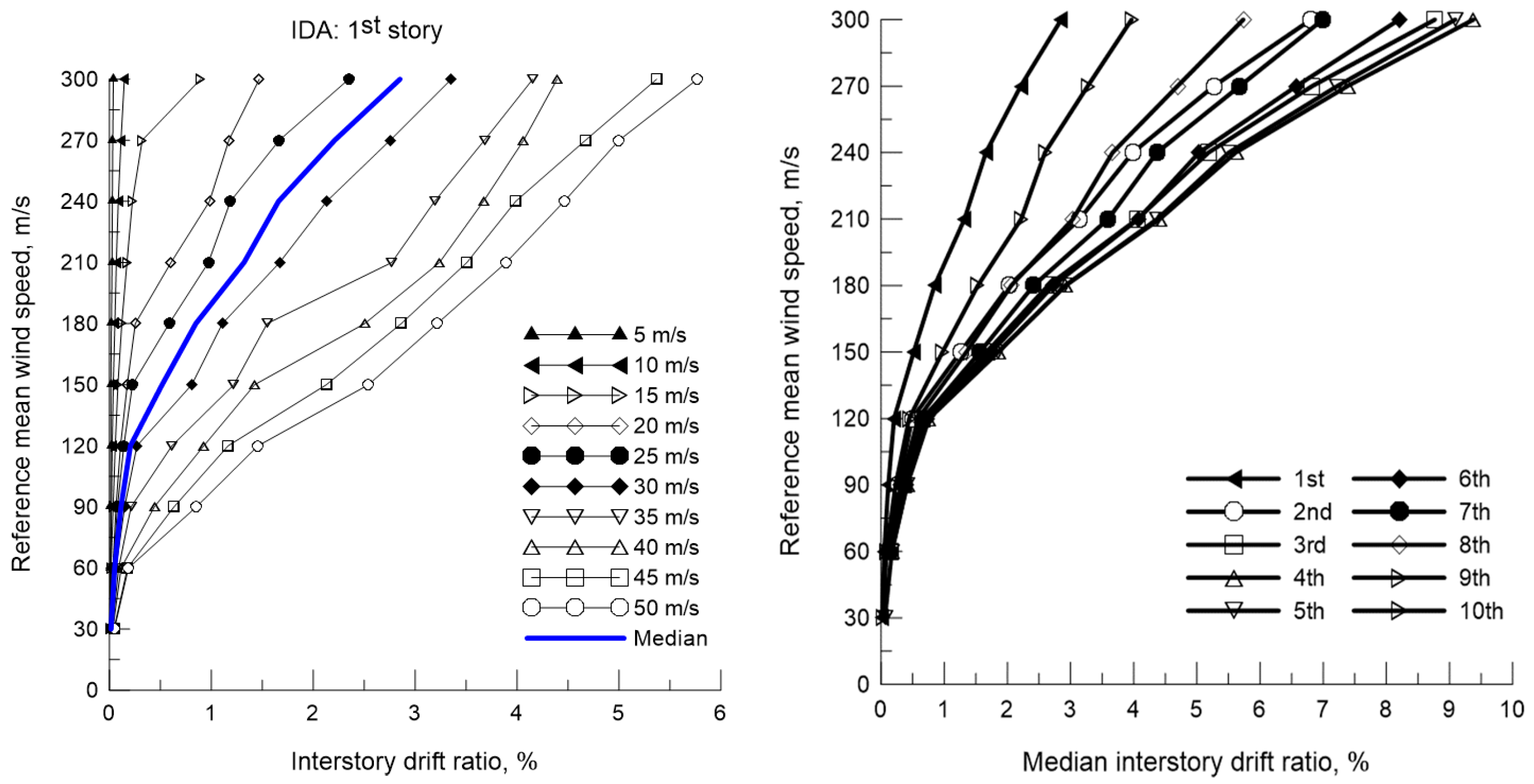
The reference ten series of wind aerodynamic loads are incremented up to a target mean reference wind speed of 300 m/s, intentionally severely overestimated. Figure 13 successively shows the first story peak drift ratio and the structural median values of the peak interstory drift ratios.

In the structural design, the interstory drift ratio is the most important parameter to control the deformability acceptance criteria associated with predefined limit states. While most of the design codes or standards provide reference interstory drifts associated with the limit states, there is no straightforward relationship with the associated damage state for a given structure. For instance, for seismic applications, the FEMA 356 Standard (2000) [25] provisions suggest acceptance criteria in terms of story drift ratios associated with three limit states as Immediate Occupancy (IO,1%), Life Safety (LS, 2%) and Collapse Prevention (CP, (4%) for RC frame structures. The acceptance criteria are incorporated in commercial software.

The correlation between median interstory drift ratios, story median damage indices and FEMA 356 (2000) [25] acceptance criteria based on 100 nonlinear dynamic analysis runs, with a one-hour duration of wind time-histories for each event, is presented in Figure 14.

Obviously, larger interstory drift leads to an increase of the story damage index. A 1% interstory drift ratio, however, corresponds to a larger median damage index than that associated with the IO limit state [25]. The interstory drift ratios at threshold limit states given by median story damage indices are in line with the suggested values given by Natural Hazards Risk Assessment HAZUS Methodology [47]. Larger design acceptance criteria values correspond to unreliable story damage indices for this case study.

These results strengthen the need of running multiple NDAs for a particular structure to control the associated damage state for various wind events from the design stage.

6. Probabilistic Wind-Induced Damage Evaluation and Loss Estimation

The Natural Hazards Risk Assessment HAZUS Methodology framework is currently used to perform probabilistic damage quantifications and loss estimations for typical structures [47,48]. Both structural capacity for lateral loads and structural demand in probabilistic terms are required data to perform wind-induced loss estimations.

The probability that a structure is in or out of a predefined damage state is efficiently provided through fragility functions. These are modelled as log-normal distributions given by the median (mean of the natural logarithm of the intensity measure (IM)) and by the log-standard deviation: the standard deviation of the natural logarithm of IM. Both parameters are currently associated in analyses based on HAZUS methodology provisions to a certain structural typology, design code level and the height regime of buildings.

The story fragility functions can thus be defined by the log-normal cumulative density function given by

$$P_k\left[ds|IM=x\right]=\Phi \left[\frac{ln\left(\raisebox{1ex}{$x$}\!\left/ \!\raisebox{-1ex}{${\theta }_k$}\right.\right)}{{\beta }_k}\right], k=1,\dots ,n-stories$$

(40)

where $\Phi$ is the standard normal distribution function, ${\theta }_k=exp(ln\left(x\right)|k)$ is the median value of intensity measure (IM), and ${\beta }_k={\sigma }_{ln\left(x\right)|k}$ is the log-standard deviation of the IM, corresponding to story (k). The IM is considered the reference mean wind speed.

The pair of story fragility curve parameters in Equation (40) are obtained based on FEMA 356 (2000) [25] provided limit states interstory drift ratios, and the Multiple Stripe Method approach (Jalayer and Cornell, 2009) [21]. Story IDA curves are artificially extended with flat lines to acquire available data for certain stories (Figure 13). The IDA approach straightforwardly provides the intra-event variability and the inter-event variability of the response as well.

The story fragility curves associated with Immediate Occupancy (1%), Life Safety (2%) and Collapse Prevention (4%) limit states are presented in Figure 15.

For the design reference mean wind speed, the structure remains elastic. For instance, for $u_{ref}=50 \mathrm{m}/\mathrm{s}$, the story probability of reaching the IO damage level reproduces the story damage index obtained by NDA. LS and CP limit states are not representative for current wind events but important for extreme ones.

Figure 16 presents the correlations between the peak median story damage indices for 3 levels of wind intensity, i.e., $u_{ref}=30, 40 \mathrm{and} 50 \mathrm{m}/\mathrm{s}$, and the associated story fragilities for IO, LS, and CP limit states.

A good correlation is observed for the largest reference mean wind speed event for the IO limit state. Low correlation for the LS limit state and no correlation for the CP limit state at the wind speeds considered are observed.

This permits the proper correlation of probabilistic story fragility with the actual damage index obtained from NDA and properly assigning interstory drift ratios associated with limit states for a given structure.

Moreover, story fragility estimates may be computed and efficiently represented in terms of increasing reference wind speed events (Figure 17).

The probabilistic fragility analyses results are further used for the estimation of structural damage cost of repair for various wind events that might occur during the service lifetime of a building. Once climatological data are available, the probabilistic wind hazard curve for a specific location can be straightforwardly used to relate the wind speed to a certain hazard level and to perform a site-dependent probabilistic analysis.

Probabilistic Estimates of Structural Damage Costs of Repair

The expected damage level or rank of a given story (k), can be computed as

$$E{D}_k={ {{\displaystyle \sum }}_{ds}{D}_{r,ds}{P}_e[ds|u_{ref}]|}_k$$

(41)

where $D_{r,ds}$ is the damage rank associated with a given damage state, and $P_e[ds|u_{ref}]$ is the probability of exceedance of that damage state obtained from the probabilistic fragility analysis. Assume that the damage rank for each damage state is 0- for the no damage state, 1- for the Immediate Occupancy damage state, 2- for the Life Safety damage state and 3- for the Collapse Prevention damage state.

Thus, the associated expected costs of damage or repair of structural components in a given story (k) can be computed by the formula

$$EC{R}_k={{{\displaystyle \sum }}_{ds}{C}_{ds}{P}_e[ds|u_{ref}]|}_k$$

(42)

where $C_{ds}$ is the cost of repair associated with a given damage state, and $P_e[ds|u_{ref}]$ is the probability of exceedance of that damage state.

Assume that the cost of repair in monetary units for each damage state is 0 units for the no damage state, 30 units for the Immediate Occupancy damage state, 70 units for the Life Safety damage state, and 100 units for the Collapse Prevention damage state.

Thus, the story expected damage rank and the associated expected repair costs for various wind events scenarios are represented in Figure 18.

The cost of repair of the overall structure is obtained simply by summing the cost of repair of individual stories. Note that neither the cost of repair of non-structural components nor the occupancy class of the building are included in the loss estimates in this study.

For current reference mean wind speeds used for design purposes, the level of structural damage and the repair costs are nearly zero. The significant damage and associated cost of repair/replacement might be primarily related to non-structural components such as façade systems, partition walls, etc.

The analysis framework entirely based on NDA is essential for resilience-based design to predict the expected damage level, the localization of damage and the associated cost of repair. The functional recovery duration is strongly dependent on this kind of information, even from the design stage. Further on, ranking the damage level and the associated repair cost for buildings in a specific exposed area will permit the development of wind-induced damage maps using the Geographical Information System (GIS) tool.

Moreover, by using a real-time vibration monitoring system and available accompanying AI-based tools, the structural damage induced by extreme wind events will be estimated by comparing the reference data provided by the designer with actual measurements. Smart building systems able to recognize a reference damage pattern provided by designers, will certainly be the next challenging target in structural engineering.

7. Conclusions

Significant progress in the performance-based design of buildings for natural hazard-induced loads, such as wind and seismic loads, is possible primarily thanks to available time-series of induced loads in conjunction with appropriate computational tools that capture the nonlinear-induced behavior and the associated expected damage.

The Force Analogy Method (FAM)-based nonlinear dynamic analysis package is briefly presented and further used as an efficient solver that yields fast and transparent time-domain response parameters for long duration aerodynamic wind loads. The use of FAM largely opens the doors for the extension of the Davenport chain for structural wind engineering applications, with analysis modules that are not required in current design practice.

For the study purposes, a large number of code-compatible wind speed testing time-series and corresponding aerodynamic wind loads were generated by using the NOWS (NatHaz on-line wind simulator) developed by NatHaz Laboratory of the University of Notre Dame, Notre Dame, IN, USA. This approach can be easily replaced by available wind tunnel pressure measurements or by Computational Fluid Dynamics (CFD)-based generated data.

Extensive time- and frequency-domain analyses of simulated time-series up to 40 m above ground level were performed to capture the input parameters that might influence the structural damage. When available, climatological data for a given site will permit the use of a probabilistic wind hazard curve (PWHC), thus relating the mean wind speed with the corresponding Mean Return Interval (MRI) of the wind event.

The numerical effectiveness of the FAM to perform fast and multiple nonlinear dynamic analyses for long duration input loads was presented. The FAM effectiveness comes first from the fact that the stiffness matrix remains constant over the entire analysis duration, while the correction of structural restoring force is performed by an analogous force vector. Secondly, a state–space formulation to solve the differential equations of motion brings additional numerical effectiveness.

The time-history response parameters and the computed hysteretic energy at each member’s section are straightforwardly and transparently used to compute the associated damage index. Both the excessive deformation and the cycling loading effects are directly accounted for. The evolution and the extent of damage at each section, member, story, and structural level are easily visualized by the structural designer for any wind event; thus, the design can be iteratively controlled in terms of allowed damage corresponding to various limit states. The analyses indicate that higher damage indices might be primarily related to larger wind gust factors, while there is no clear evidence on the effect of turbulence intensity on the structural damage state.

The Incremental Dynamic Analysis (IDA) based on FAM is further used to obtain dynamic story pushover curves. Story fragility curves for three limit states currently used were constructed using the multiple stripe method and available interstory drift ratios provided in the literature. The correlation between the interstory drift ratio and the associated story damage index, obtained from a very large number of nonlinear dynamic analyses for different wind scenarios, needs to be further considered for setting up the limit states for a particular structural system.

Expected damage levels and associated structural cost of repair are lastly provided by the analyses for various wind events as an essential component of a future resilience- based analysis and design framework.

The results using testing functions of simulated wind loads on a typical frame model are encouraging for the implementation of a complete performance-based design framework for wind loads in a unified multi-hazard approach, including seismic and wind engineering applications.

The proposed integrated analysis framework next requires extension to tridimensional models able to transparently capture the wind directionality effect and straightforwardly integrate the wind tunnel measurements or the CFD-based pressure data corresponding to extreme synoptic and non-synoptic wind events.

Moreover, the structural damage evaluation is to be further used as reference analysis-based data for damage pattern recognition from real-time vibration measurements and AI-based damage recognition algorithms.