An Experimental Study of Non-Gaussian Properties of Tornado-like Loads on a Low-Rise Building Model

Abstract

This paper focuses on the non-Gaussian properties of tornado pressure loading on a Texas Tech University (TTU) building model. External pressures of the model were measured at multiple radial positions in a two-celled tornado-like vortex generated by a tornado-like vortex simulator. High-order statistical moments of pressure coefficients were studied. The spatial distributions of non-Gaussian zones were presented and compared with the figure for boundary layer wind. Four exponential models were used to fit the probability density of tornado pressures. The peak factors obtained by five methods were also investigated. Results indicate that non-Gaussian regions of a low-rise building in a tornado-like vortex significantly differ from that in boundary layer wind. The peak pressure coefficients exhibit a maximum value near the end of windward eaves when the model is located at a tornadic core radius. The probability density of tornado pressure time series cannot be fitted by a single exponential distribution. The gamma distribution and generalized extreme value (GEV) distribution can describe the probabilistic behavior of pressure coefficients at the most unfavorable load position. Compared with other methods, the skewness-dependent peak factor method exhibits the advantages of reliable results, easy calculation, and wide applicability.

1. Introduction

With the increasing sophistication of wind load theories, researchers have realized that the non-Gaussianity of wind pressures is an important issue that must be considered in the structural design work. In flat regions of a structure’s surface, the spatial correlation of the flow field decays rapidly, and the wind pressures in these areas tend to be subject to Gaussian fluctuations. In regions of corners or regions with an abrupt change in shape, however, the pressures tend to be subject to non-Gaussian fluctuations due to the vortices generated by flow separation. The probability density distribution of wind pressure in non-Gaussian regions is generally asymmetric, with a long-tail side, which means non-Gaussian wind pressures may be accompanied by large pluses that could be more likely to cause damage to the structure.

The main research directions of non-Gaussian wind loads can be summarized as follows. The first is the non-Gaussian zone. Kumar et al. [1] conducted a series of wind tunnel tests on low-rise buildings with flat roofs, gable roofs, and mono-slope roofs, respectively, as shown in Figure 1. The non-Gaussian zones of the three types of buildings for an azimuth of 0°–90° were studied, based on the skewness and kurtosis of the pressure time series. Caracoglia et al. [2] carried out a long-term field measurement on a typical structure located near the coast of North Carolina and analyzed the skewness and kurtosis of different zones. Liu et al. [3] recorded the external pressures on the roofs of some buildings in Florida during the landfall of a hurricane and presented the high-order statistical moments and probability density of pressure time series data. The results of the wind tunnel test were also compared with the field measurement data. The conclusions of these studies on low-rise buildings are similar. (1) For gable roofs, non-Gaussian zones are located on the ridge and eave and (2) for flat roofs, non-Gaussian zones are located on the windward eave. (3) The contour maps of skewness and kurtosis in wind tunnel tests are similar in shape but different in value compared with the field measurement results.

The second is the probability model of wind pressure. Early studies were mainly devoted to finding the most suitable to fit the probability density function (PDF) of non-Gaussian wind pressures from the traditional exponential distributions. Tieleman and Reinhold [4] attempted to utilize non-Gaussian distributions to fit the probability density of wind pressure. They calculated that the Weibull distribution was acceptable. Gioffrè [5], Sadek, and Simiu [6] and Quan et al. [7] found that the lognormal distribution, hamma distribution, and GEV (generalized extreme value) distribution were the appropriate models for the fitting of wind pressure histograms, respectively. The application ranges of traditional exponential distributions are different from each other, which accounts for the discrepancy between the research mentioned above. Considering the exponential distributions only involve the first three statistical moments at most, many researchers turned to utilize other mathematical models, such as the hermit polynomial model (HPM), to translate the non-Gaussian process into the Gaussian process, thereby fitting the probabilistic behavior of non-Gaussian wind pressures [8,9,10]. Based on the translation process theory, these methods proved superior to the traditional exponential distributions in fitting the PDF of non-Gaussian wind pressures precisely and estimating the extreme value of wind loads. However, it does not mean that the traditional exponential distributions are out-of-date. Apart from the advantages of easy calculation and concise expression, the exponential distributions could also represent some statistical properties of the data.

The third is estimating the extreme values of wind loads. Davenport [11] proposed the Gaussian peak factor method, assuming that the wind pressure time series is a Gaussian process. However, local pressures in flow separation regions could severely deviate from Gaussian distribution, which results in the extreme values obtained by the Davenport method usually being smaller than the actual values. Many researchers have been trying to extend the Davenport method to the non-Gaussian region, among which the most widely accepted are the methods of Kareem–Zhao and Sadek–Simiu. Sadek and Simiu [6] obtained the CDF (cumulative distribution function) of peaks by using the translation process approach. The extreme value could be estimated by calculating the expectation of peaks. Kareem and Zhao [12] applied the HPM to transform the Gaussian random variables into a polynomial of non-Gaussian random variables which contained higher-order statistical moments (skewness and kurtosis), thereby modifying the Davenport peak factor. On the basis of Kareem–Zhao, some researchers [13,14] have argued that the non-Gaussian peak factor is mainly determined by skewness coefficients, arguing that kurtosis contributes little to it. Lin et al. [15] proposed a skewness-dependent peak factor method. They simplified the effect of kurtosis to an empirical constant so that the method is available in the whole Pearson map.

Although the studies on the non-Gaussian properties of wind loads have made much progress, all of them are based on the premise that the incoming flow is synoptic wind. The figure for non-synoptic wind, such as tornadoes and downbursts with significantly different wind profiles and turbulent properties from normal wind, still remain unknown. Recently, tornados have received a great deal of attention from researchers for their great destructiveness. In China, tornadoes have caused some severe disasters with significant casualties and huge material loss [16], such as the sinking of the Easter Star cruise ship in June 2015, the Jiangsu tornado disaster in June 2016, and so on. The frequency of tornado disasters is also on the rise for the past few years. It was reported that four tornadoes had attacked the north of Jiangsu Province on 20 July 2022. Tornadoes tend to occur in a terrain that is flat and open, such as suburban and rural areas where there are a large number of low-rise buildings. Therefore, it is valuable and urgent to reveal the mechanism of tornado damage to low-rise building structures and to propose reliable methods for structural safety design. Research related to earthquake resistance and wind-induced vibration focuses more on the response of structures to loads [17], while research related to tornadoes focuses more on the loads acting on structures. Most of the current studies on tornado-induced loads are conducted to work out the effects of various factors on the mean value of tornado load; for instance, the opening ratio [18], building type [19,20], swirl ratio [21], tornado moving speed [22], etc. Few studies are related to the non-Gaussian properties and extreme value estimation of tornado loads, except for Tang et al. [23], who measured the external pressure coefficients on two rectangular prisms in tornadic wind tunnel tests and presented contours of the first four statistical moments.

To advance the understanding of the non-Gaussian properties of tornado pressure loading on low-rise buildings with rectangular shapes, an experimental study on a TTU building model was carried out in this paper. The external pressures of the model were measured at multiple radial locations in a two-celled tornado-like vortex generated by a Tongji University (TJU) tornado simulator. The higher-order statistical moments of tornado pressure coefficients, the PDF of the tornado pressure, and the methods of estimating the extreme value of tornado loads were investigated.

2. Experimental Setup

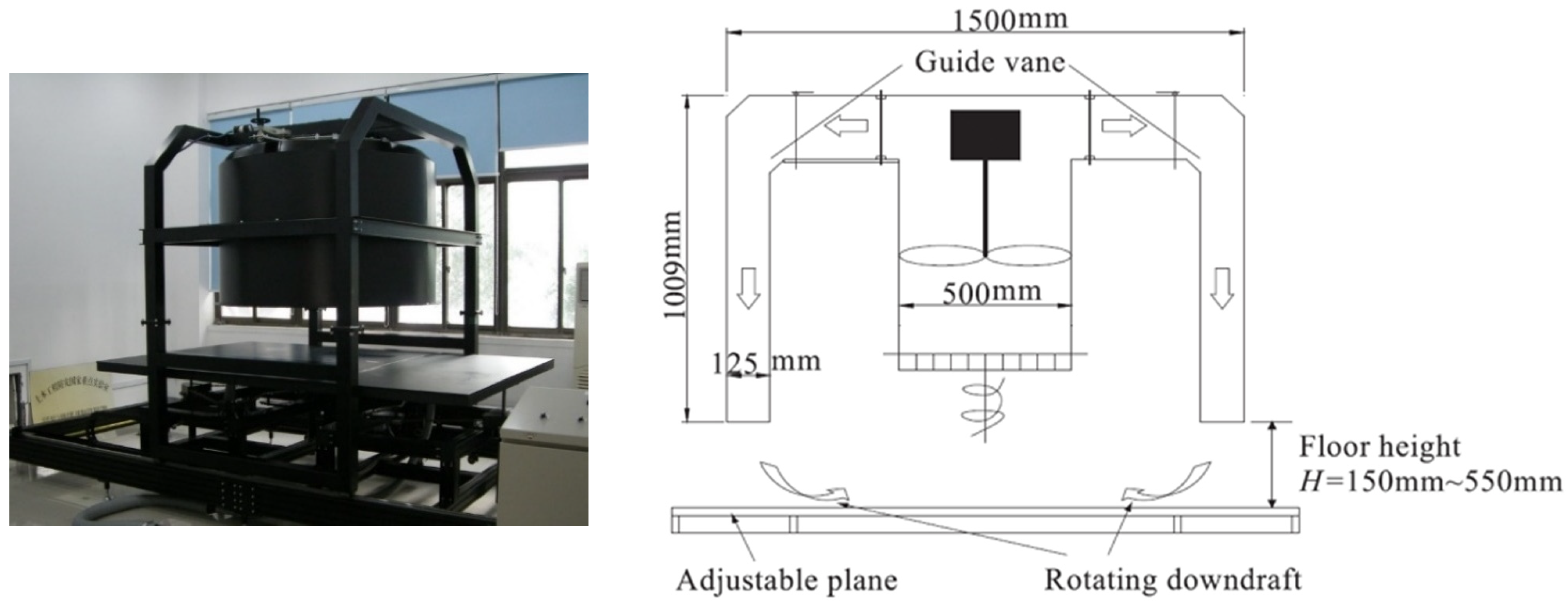
2.1. Tornado Simulator

The tornado simulator of Tongji University [22], as shown in Figure 2, was utilized in the present study. The mechanism for generating the tornado-like vortex is similar to that at Iowa State University (ISU), USA [24]. This simulator could produce both stationary and translational tornado-like vortices. The updraft, generated by controlling the fans, passes through the guide vane and the outer cylinder wall to form a tornado-like vortex between the platform and the honeycomb. The platform is open-ended, on which the model can be placed. A tornado-like vortex with different swirl ratios and scales can be obtained by changing the angle of the guide vane, the height of the incoming flow, and the speed of the fan of the simulator.

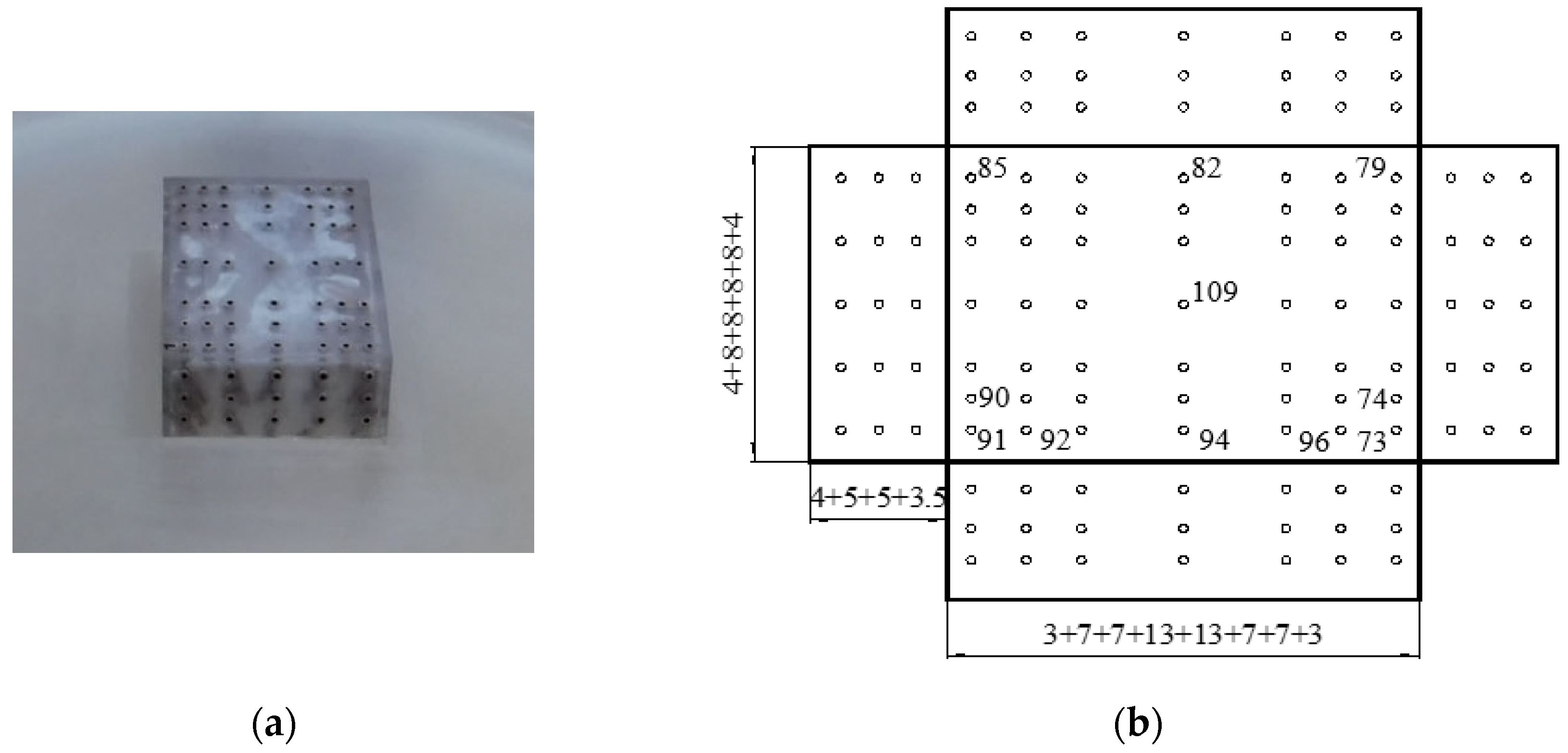
2.2. Building Model and Test Configurations

Experimental testing was conducted on a TTU building model with a total of 121 pressure taps, as indicated in Figure 3.

Table 1. Building model parameters.

Parameter	Value
Roof type	Flat 1
Length	60 mm
Width	40 mm
Depth	17.5 mm
Length scale	1:300
Velocity scale	1:5
Time scale	1:60

¹ Actually, the original TTU building model has a roof angle of 6°. In this test, the model is too small that its roof angle can be ignored.

provides a summary of detailed information regarding the building model parameters. The length scale adopted for the study was based on the ratio of the simulated tornado core radius to the actual tornado core radius. In China, typical tornadoes have a core radius ranging from 20 m to 50 m, which translates to a length scale range of 1:300 to 1:800. Considering that a smaller model can lead to processing difficulties, it is advisable to use a larger length scale factor. Therefore, a length scale of 1:300 was deemed reasonable. The velocity scale was determined by comparing the maximum mean tangential velocity of the simulated tornado with that of an actual tornado. The test aimed to simulate an EF2-EF3 tornado with a velocity range of 50 m/s–74 m/s, as shown in

Table 2. Enhanced Fujita scale of tornadoes.

EF Scale	EF0	EF1	EF2	EF3	EF4	EF5
Wind velocity (m/s)	29–38	39–49	50–60	61–74	75–89	>89

. Hence, a velocity scale of 1:5 was selected in the study.

The location of building model (x) with different building azimuths (θ) was changed along the centerline of the stationary tornado, with one side wall normal to the tangential flow, as shown in Figure 4.

Table 3. Test parameters.

Parameter	Value
x/mm	0, ±10, ±20, ±35, ±50, ±60, ±70, ±80, ±90, ±100, ±110, ±120, ±140, ±160, ±180, ±210
θ/°	0, 90

summarizes the 31 radial positions and 2 building azimuths. A tornado-like vortex in this test was counter-clockwise. It should be noted that the windward wall of the model is not always fixed due to the unique rotating three-dimensional structure of tornado flow. The windward wall at x > 0 would become leeward when x < 0.

2.3. Measurements and Data Processing

Two turbulent flow instrumentation (TFI) Cobra probes were used for wind velocity measuring. A multi-channel pressure measuring system at a sampling frequency of 300 Hz was used for recording the pressure time series of the model surface, and the sampling time was 60 s. The distortion of pressure signals caused by the tube system was corrected through the frequency response function.

The pressure coefficient of a tap is defined in Equation (1):

$$C_p(t)=\frac{P(t)-P_{ref}}{0.5\rho U_{t,\max }^2}$$

(1)

where $P(t)$ is the local pressure, $P_{ref}$ is the reference atmospheric pressure far from the tornado-like vortex, $\rho$ is air density, and $U_{t,\max }$ is the maximum tangential velocity of the tornado-like vortex. $C_{\mathrm{p}\_\mathrm{peak}}$ is the peak value of $C_p(t)$.

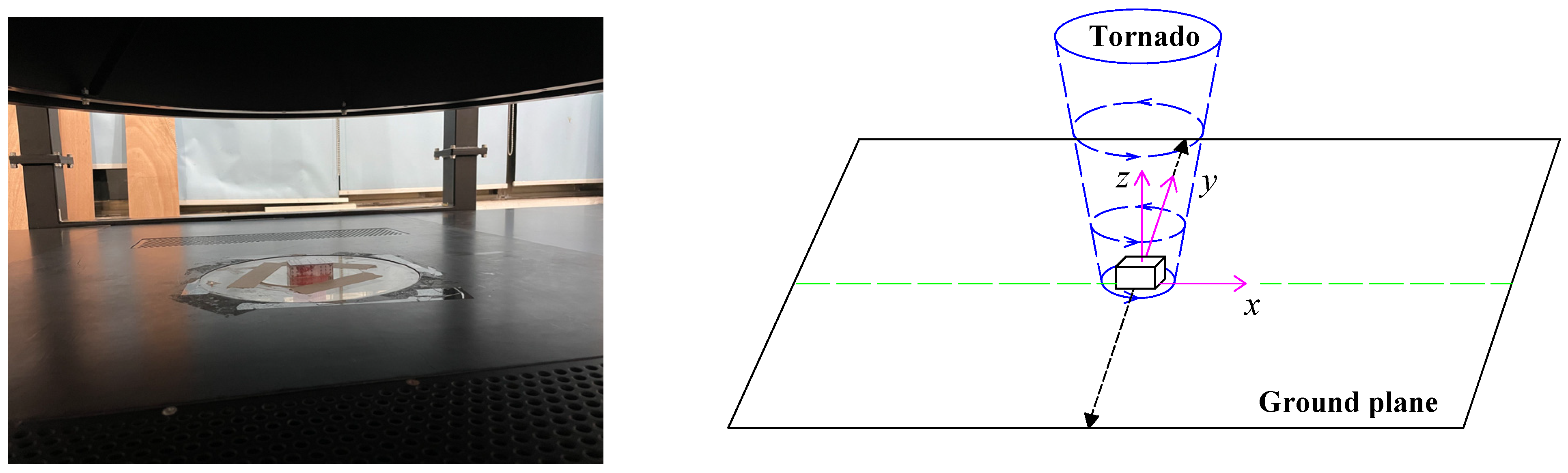
3. Tornado-like Vortex

According to the study by Lewellen et al. [21], the swirl ratio, whose physical meaning is the ratio of angular momentum to total inflow rate, is the central parameter of the structure of the tornado-like vortex. In a tornado simulator, the swirl ratio can be estimated by Equation (2):

$$S_r=\frac{r_0}{2H}\cdot \tan {\theta }_v$$

(2)

where $r_0$ is the radius of the updraft, equal to the radius of the inner cylinder, taken as 250 mm, $H$ is the inflow height, and ${\theta }_v$ is the angle of the guide vane. Wang et al. [22] and Wang et al. [25] found that when the swirl ratio is >0.5, a single-vortex tornado-like flow gradually breaks down and develops into a multi-vortex structure. In order for the tornado-like wind field to be significantly different from the synoptic wind field, a large swirl ratio of 0.74 was selected in this test. The inflow height is $H$ = 200 mm, the guide vane angle is ${\theta }_v$ = 50°, and the fan speed is 1500 RPM.

Two Cobra probes were placed symmetrically along the central line of the tornado simulator’s center, as shown in Figure 5. Adjust the radial locations and elevations above the ground plane of the Cobra probes to capture the information of the tornado-like field. The mean tangential velocity $V_t$, mean radial velocity $V_r$, mean axial velocity $V_a$, and pressure drop $P$ at certain heights were presented in Figure 6. It can be seen that in a horizontal plane, as shown in Figure 6a, the mean tangential velocity increases rapidly to its peak, followed by a slow decrease, with an overall M-shaped distribution. The horizontal distance between the location where the maximum mean tangential velocity occurs and the center of the tornado simulator is called the core radius, denoted as $r_c$. The absolute value of pressure drop fluctuates within the central area of the tornado-like vortex and then decreases rapidly with the increasing distance from the center. The fluctuations of pressure drop in the central area indicated that the tornado-like vortex developed into multi-vortices; if not, the central part of the pressure drop would be sharp for a single-vortex structure. Compared with tangential velocity, radial velocity and axial velocity account for a low proportion of the total velocity. The distributions of velocities were not strictly centrosymmetric, which may be caused by the vortex drift of the tornado itself. Detailed information on the tornado-like field was summarized in

Table 4. Parameters of the tornado-like vortex.

Parameter	Value
Swirl ratio Sr	0.74
Maximum tangential velocity Ut, max	13.4 m/s
Height at which Ut, max occurs hc	15 mm
Radius at which Ut, max occurs rc	70 mm

.

4. Results and Discussion

4.1. Non-Gaussian Zone

A particular region is considered non-Gaussian if the absolute values of skewness and kurtosis are >0.5 and >3.5, respectively [1]. Figure 7 shows the skewness and kurtosis of the roof taps at model positions from x = −3r_c to x = 3r_c. The range between the two horizontal dashed lines represents the Gaussian region. It can be seen in Figure 7 that the skewness and kurtosis of most taps are in the non-Gaussian region when x is around 0. As x increases, the distributions of skewness and kurtosis become more dispersed. Some taps gradually back to the Gaussian region, while some extreme values also show up. Additionally, the numbers of positive skewness or negative excess kurtosis also increase with x, which is rare in normal wind loads. The maximum skewness and kurtosis occur near x = 2r_c.

For a more visual understanding, Figure 8 shows the approximate Gaussian zones and non-Gaussian zones at different positions and building azimuths, and the results of an atmospheric boundary layer (ABL) wind tunnel test (Kumar et al. [1]) are given for comparison. When x is within 0.5 r_c, as shown in Figure 8a,b,e,f, most areas of the structure’s surface are subjected to non-Gaussian fluctuations. As x increases to r_c and 2r_c, the windward edges of the roof are subjected to Gaussian fluctuations and the middle portion of the roof is subjected to non-Gaussian fluctuations, which is the exact opposite of the ABL results.

Researchers have reached a consensus on the causes of non-Gaussian wind pressure, which is the turbulence of the incoming flow and the micro-vortices generated by flow separation. In view of the fact that the tornado vortex is always drifting around the central axis with a high speed, is not fixed, and the wind velocity in the center of the tornado vortex is relatively small, it can be inferred that the non-Gaussian zone of the model at x = 0 is mainly caused by the fluctuations of the tornado’s own pressure drop. At x = r_c, the tangential wind velocity increases to a maximum and generates a stable vortex, which happens to reduce the non-Gaussianity brought by pressure fluctuations. This may explain why the windward sides of the model in a tornado-like vortex are likely to suffer from Gaussian wind pressures. In addition, the wind profiles of a tornado-like vortex and the ABL wind are also significantly different from each other, as shown in Figure 9. The wind profile is normalized by the height of model eaves z₀ and the wind velocity u₀ at model eaves. For the tornado-like vortex at x = r_c, the maximum wind velocity occurs within the building height and then decreases with increasing height. The unique wind profile for the tornado-like vortex must result in a distinct aerodynamically induced pressure and bring changes into the flow separation area of the building surface. The connection between the building size effect and non-Gaussian zones needs to be further studied.

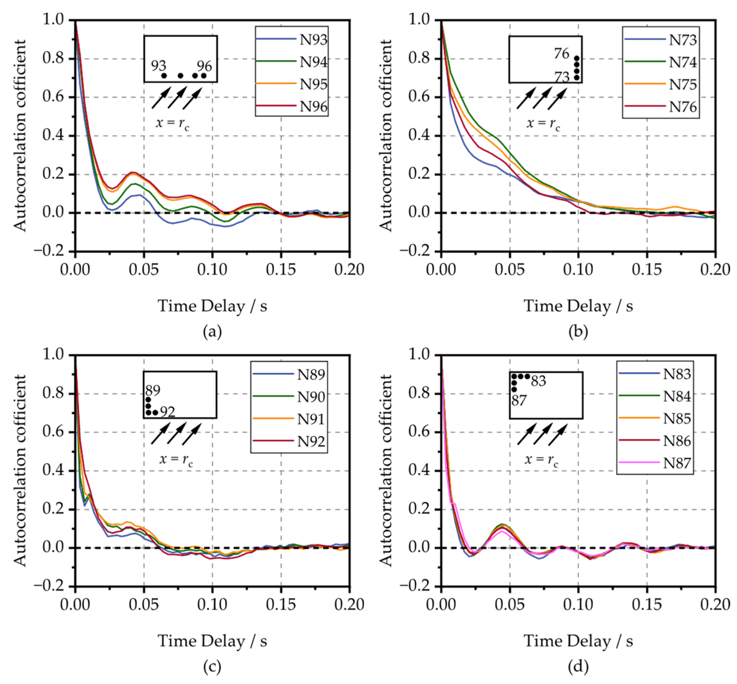
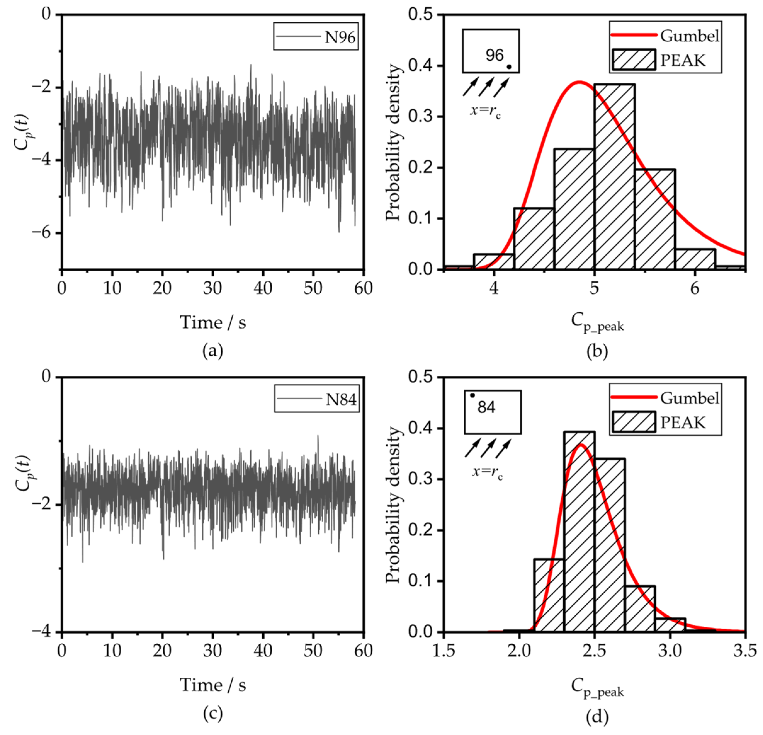
4.2. Extreme Value Estimating of Tornado-like Pressure

According to the classical extreme value theory, for a large number of independent identically distributed samples, their peak values can possibly be presented by any one of the extreme value distributions: Type I, II, or III. For wind loads, Type I, also called the Gumbel distribution, can describe the probability density of its extreme values. The general expression for the cumulative density function (CDF) of the Gumbel distribution is:

$$F_X(x)=\exp \{-\exp [-(x-\mu )/\beta ]\}$$

(3)

where μ is the location parameter and β is the scale parameter. The expectation and standard deviation of the extreme values are:

$$\overline{x_e}=\gamma \cdot \beta +\mu$$

(4)

$${\sigma }_{x_e}=\frac{\pi }{\sqrt{6}}\cdot \beta$$

(5)

where γ = 0.5772, the Euler constant. However, to fit the Gumbel distribution requires an extremely large number of samples, i.e., a lot of wind tunnel tests or field measurements, which is very uneconomical for wind tunnel tests or field measurements. Therefore, Quan et al. [27] proposed an improved Gumbel method to extract more information from a small number of samples, which was adopted in this paper to calculate the extreme values of tornado loads. On the premise that the samples are independent of each other, they derived the parameter by converting the equation between short and long time intervals:

$$\beta (T=t_1)=\beta (T=t_2)$$

(6)

$$\mu \left(T=t_1\right)=\mu (T=t_2)+\beta (T=t_2)\cdot \ln (t_1/t_2)$$

(7)

where t₁ is the long time interval and t₂ is the short time interval. The steps of the improved Gumbel method are as follows:

• Analyze the autocorrelation function of the original sample and find the time delay when the autocorrelation coefficient drops from 1 to near 0;
• Determine an appropriate time interval t₂ and divide the original sample into subsamples at intervals of t₂;
• Utilize the Gumbel distribution to fit the distribution of the maximum values of the subsamples and obtain parameters $\mu (T=t_2)$ and $\beta (T=t_2)$;
• Convert $\mu (T=t_2)$ and $\beta (T=t_2)$ into $\mu \left(T=t_1\right)$ and $\beta (T=t_1)$ using Equations (6) and (7);
• Calculate the expectation of extreme values using Equation (4) with parameters $\mu \left(T=t_1\right)$ and $\beta (T=t_1)$.

Figure 10 shows the autocorrelation coefficients of serval roof taps located in four different regions when x = r_c. It can be seen in Figure 10 that the autocorrelation functions of the taps located in the same region have similarities in shape and decay rate. From the microcosmic, this phenomenon indicates that these taps located in the same region are very likely under the same vortex. Although N96 and N73 are next to each other, the decaying trend of their autocorrelation functions looks completely different. That is because the radial wind velocity reached its peak at x = r_c, which could not be neglected. Therefore, the short eave (N73-N76) opposite to the radial flow should also behave as a windward side in the long eave (N93-N96) that was facing the tangential flow, resulting in different aerodynamically induced pressures for each eave. All the autocorrelation functions in Figure 10 are stable around 0 before 0.2 s, so the short time interval t₂ is taken as 0.2 s. Figure 11 shows the distribution of peak values from samples divided by 0.2 s and illustrates that the Gumbel distribution can fit the tornado extreme value distribution.

Since the tornado-like flow in this test is stationary, it should be regarded as a quasi-steady flow. The observation time interval is taken as 10 min, so the scale time interval t₁ is 10 s. In order to study the most unfavorable tornado loads, a contour plot with the maximum $C_{\mathrm{p}\_\mathrm{peak}}$ occurring from x = −3r_c to x = 3r_c is shown in Figure 12, where $C_{\mathrm{p}\_\mathrm{peak}}$ is calculated by the improved Gumbel Method. For $\theta =0°$ and $\theta =90°$, the maximum $C_{\mathrm{p}\_\mathrm{peak}}$ at the taps located on eaves, roofs, and corners are greater than that located in other areas, and the most unfavorable load occurs near the end of the eave. Taps near the most unfavorable load position are picked up for further study. Figure 13 shows the pressure coefficients at certain taps and their variations with the model’s position. From x = −3r_c to x = r_c, $C_{\mathrm{p}\_\mathrm{peak}}$ at all the taps shows an overall increasing trend and reaches the peak at around x = r_c. This is because the tangential wind velocity also reaches the maximum at x = r_c and generates a strong negative pressure on the windward eaves due to the flow separation. The most unfavorable tornado pressure coefficients for $\theta =0°$ and $\theta =90°$ are 7.51 (N96) and 6.45 (N90), respectively.

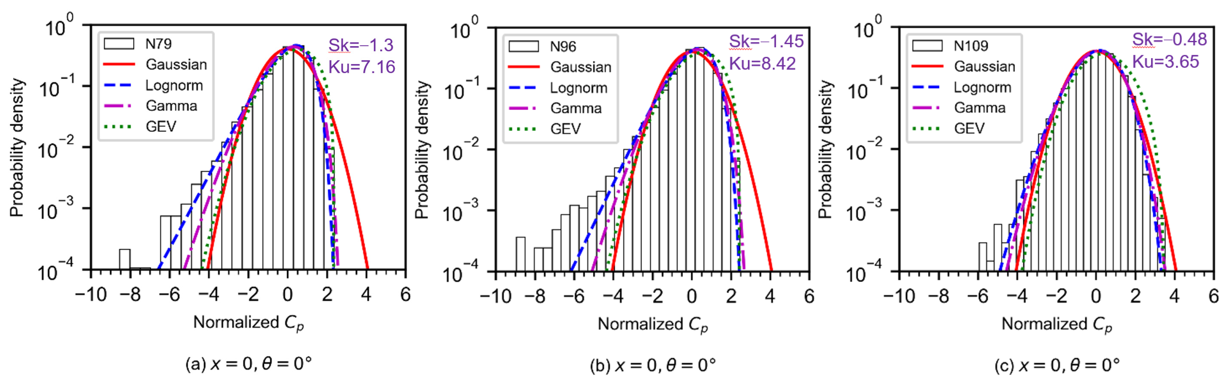
4.3. Probability Density Function of Tornado Pressure Time Series

As mentioned above, the tornado-like flow in this test should be regarded as a quasi-steady flow, which means the time series can be assumed as an ergodic and stationary stochastic process. Accordingly, a probability density function that does not vary with time is capable of describing the probabilistic behavior of tornado loads. In this section, several commonly used exponential distributions are chosen to fit the probability density distribution of tornado pressures.

• The Gaussian distribution:

$$f(x)=\frac{1}{\sqrt{2\pi }\sigma }\exp [-\frac{{(x-\mu )}^2}{2{\sigma }^2}]$$

(8)

where $\mu$ and $\sigma$ are the mean and standard deviation, respectively.

• The 3-parameter lognormal distribution:

$$f(x)=\{\begin{array}{c}\frac{1}{\sqrt{2\pi }\sigma (c-x)}\exp \{-\frac{1}{2{\sigma }^2}{[\ln (c-x)-\mu ]}^2\},x<c\\ 0,x\ge c\end{array}$$

(9)

where c is the third parameter, estimated from the samples, $\mu$ is the mean, and $\sigma$ is the standard deviation of $\ln (c-x)$.

• The 3-parameter gamma distribution:

$$f(x)=\{\begin{array}{c}\frac{1}{{\beta }^{\gamma }\mathsf{\Gamma }(\gamma )}{(x-\mu )}^{\gamma -1}\cdot \exp (-\frac{x-\mu }{\beta }),x>\mu \\ 0,x\le \mu \end{array}$$

(10)

where $\beta$, $\gamma$, and $\mu$ are the scale, shape, and location parameters, respectively, and $\mathsf{\Gamma }(.)$ is the gamma function.

• The GEV (generalized extreme value) distribution:

$$f(x)=\frac{1}{\beta }\exp [-{(1+\xi \cdot \frac{x-\mu }{\beta })}^{-1/\xi }]\cdot {(1+\xi \cdot \frac{x-\mu }{\beta })}^{-(1+1/\xi )}$$

(11)

where $\beta$, $\xi$, and $\mu$ are the scale, shape, and location parameters, respectively. When $\xi$ = 0, Equation (11) would degenerate into Type I extreme value distribution.

The probability density of normalized pressure coefficients of three taps (N79, N96, and N109) at different model positions (x = 0 and x = r_c) are fitted by the four distributions. In order to show the fit of long-tailed sides, the y-axes in Figure 14 are set to logarithmic. It can be seen in Figure 14 that the probability density of tornado pressure shows a negative skew distribution. At x = 0, all the mathematical models cannot fit the long-tailed side. Relatively speaking, the lognormal distribution is the better one. This illustrates that the relationship between the skewness and kurtosis at x = 0 is not in the application range of the GEV and gamma distributions. For pressure coefficients at the three taps, the non-Gaussianity is weaker than that at x = 0, and both the GEV and gamma distribution can fit it well. The difference between the GEV and Gamma distribution is that the former fits short-tailed sides better, while the latter fits long-tailed sides better. It is worth mentioning that the tornado loads reach a maximum at x = r_c, especially for N96, which represents the most unfavorable load position. The structural design of the tornado load is based on the assumption that the PDF of the tornado pressure is the GEV or gamma distribution, which is practical.

4.4. Comparison of Different Peak Factor Methods

There are two main theories for calculating the extreme value of wind loads. One is the classical extreme value theory, which has been introduced in Section 4.2. The other is the zero-crossing rate theory, which has been introduced in Section 1. In this section, four methods based on zero-crossing rate theory are chosen to calculate the peak factors of tornado loads at x = r_c, and the results are compared with that of the improved Gumbel method.

The error ratio is defined as:

$$\mathrm{error} \mathrm{ratio}=\frac{\mathrm{Calculated} \mathrm{Value}-\mathrm{Standard} \mathrm{Value}}{\mathrm{Standard} \mathrm{Value}}$$

(12)

The standard value is the extreme pressure coefficients calculated by the improved Gumbel method, while the calculated value is the figure for other peak factor methods. During the calculation, the parent distribution in the Sadek–Simiu method is the gamma distribution. It can be seen in Figure 15 that the Gaussian peak factor method has the largest negative deviation from the standard value. The results of the Sadek–Simiu method show large error ratios at some taps, exceeding 0.3, and the error ratio for the rest taps fluctuates around 0.1. As analyzed in Section 4.3, the gamma distribution cannot fit well at the taps with strong non-Gaussianity, which leads to inaccuracy in estimation. The methods of Kareem–Zhao and Lin et al. are the closest to the standard value. The extreme values of the Kareem–Zhao method are larger than the standard value, while that of Lin’s method are smaller. The error ratios of the Lin et al. method were smoothly distributed within 0.1, which is more concentrated than that of the Kareem–Zhao method. In addition, it can be found in Figure 15 that there are null values for the Kareem–Zhao method; for example, the tap N73. That is because the relationship between skewness and kurtosis at a certain location does not satisfy the prerequisite for using the HPM. The Lin et al. method does not have to take this into account since the effect of kurtosis has been simplified to a constant. Compared with the Kareem–Zhao method, the Lin et al. method has the advantages of more stable results, a wider range of applications, and being easier calculate. Compared with the improved Gumel method, the Lin et al. method requires a smaller sample size. Therefore, the skewness-dependent peak factor method proposed by Lin et al. is the better way to estimate tornado loads.

Engineers are used to estimating the extreme wind load through the peak factor. Tornado peak factors calculated by all the methods mentioned in this paper are summarized in

Table 5. Summary of peak factors obtained by different methods.

Model Position	Tap Number	Method	Value
x = rc	N96	Improved Gumbel Method	5.6
x = rc	N96	Gaussian Peak Factor Method	3.6
x = rc	N96	Sadek–Simiu Method	4.4
x = rc	N96	Kareem–Zhao Method	5.2
x = rc	N96	Lin Method	5.1

. The most unfavorable load position, N96 at x = r_c, is further confirmed, and the peak factors given by methods based on zero-crossing rate theory are less than the improved Gumbel method. For the TTU building model, a tornado peak factor of 5.6 is relatively safe.

5. Conclusions

In this study, the external pressures of a TTU building model at different positions in a tornado-like vortex were measured, followed by a comprehensive analysis of non-Gaussianity in tornado pressures. The conclusions are listed below:

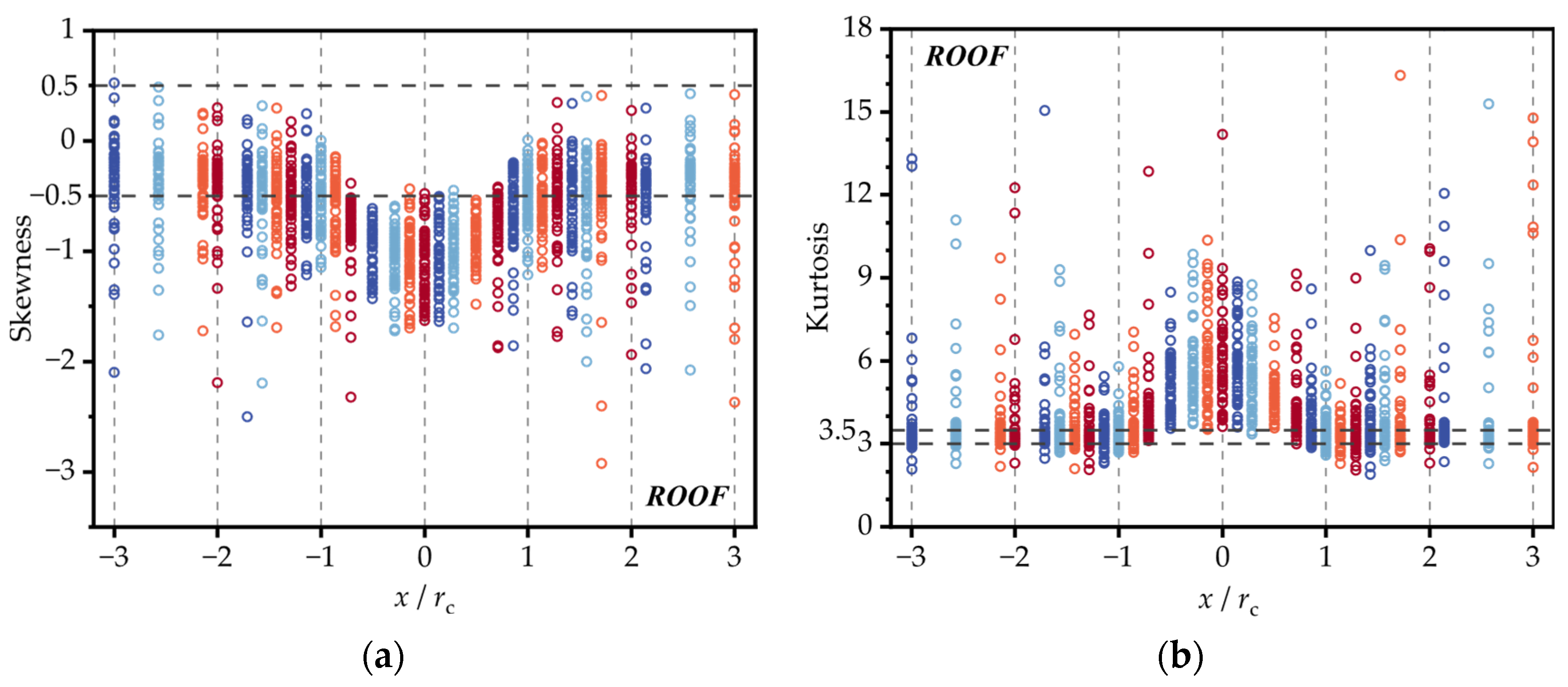
• At the center of the tornado vortex, the skewness and kurtosis of roof taps are uniformly distributed in a small range, and almost all of the model’s surface is subject to non-Gaussian fluctuations. At the core radius of the tornado vortex, for taps with different spatial locations, their skewness and kurtosis vary greatly from each other. The windward walls and eaves are subject to Gaussian fluctuations, while the middle portion of the roof is subject to non-Gaussian fluctuations.
• The PDF of tornado pressure time series on the surfaces of the buildings cannot be fitted by one certain exponential distribution, especially in the regions of strong non-Gaussianity. Compared with Gaussian distribution and lognormal distribution, the GEV distribution and gamma distribution are the better mathematical models to describe the probability density of tornado pressures at the most unfavorable load position.
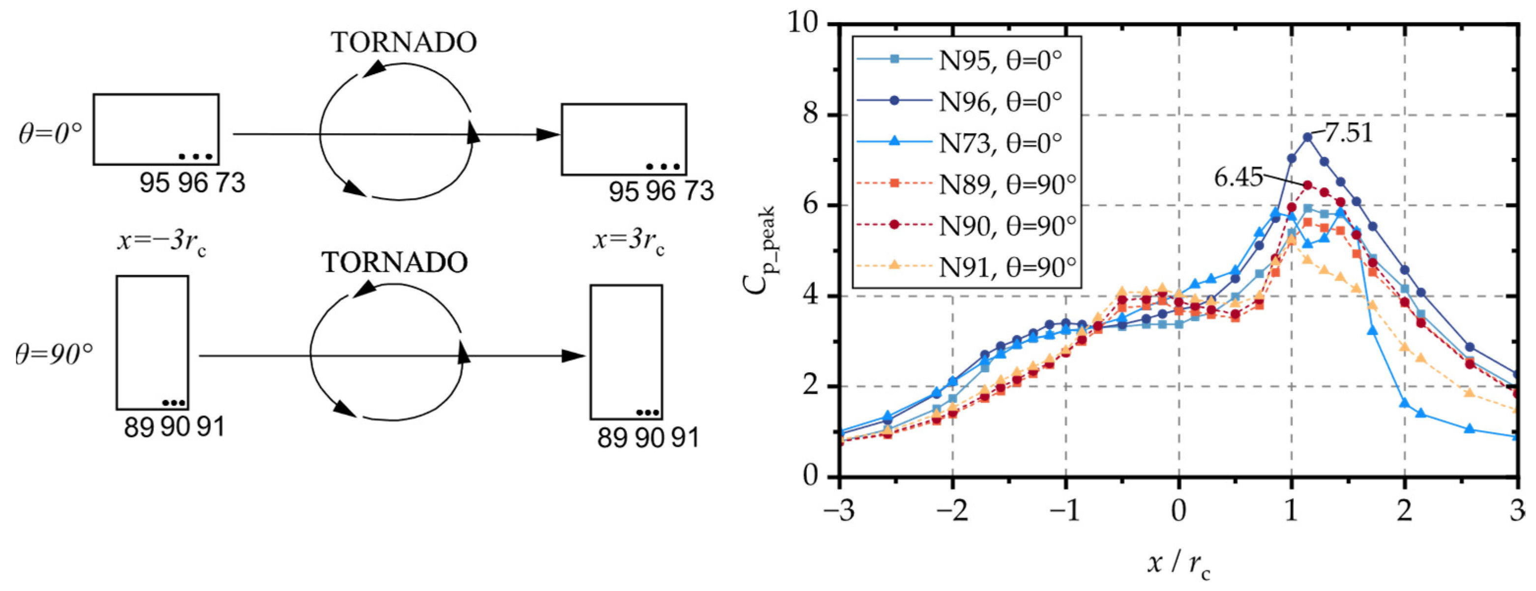
• The skewness-dependent peak factor method is the better way to estimate the tornado loads. For a TTU building model in a tornado-like vortex with a swirl ratio of 0.74, the most unfavorable load position is near the end of windward eaves, and the tornado peak factor can be relatively safely taken as 5.6.

References

1. Kumar, K.S.; Stathopoulos, T. Wind Loads on Low Building Roofs: A Stochastic Perspective. J. Struct. Eng. 2000, 126, 944–956. [Google Scholar] [CrossRef]
2. Caracoglia, L.; Jones, N.P. Analysis of Full-Scale Wind and Pressure Measurements on a Low-Rise Building. J. Wind Eng. Ind. Aerodyn. 2009, 97, 157–173. [Google Scholar] [CrossRef]
3. Liu, Z.; Prevatt, D.O.; Aponte-Bermudez, L.D.; Gurley, K.R.; Reinhold, T.A.; Akins, R.E. Field Measurement and Wind Tunnel Simulation of Hurricane Wind Loads on a Single Family Dwelling. Eng. Struct. 2009, 31, 2265–2274. [Google Scholar] [CrossRef]
4. Tieleman, H.W.; Reinhold, T.A. Wind Tunnel Model Investigation for Basic Dwelling Geometries; Department of Engineering Science & Mechanics: Virginia Polytechnic, VA, USA, 1976. [Google Scholar]
5. Gioffrè, M.; Gusella, V.; Grigoriu, M. Non-Gaussian Wind Pressure on Prismatic Buildings. II: Numerical Simulation. J. Struct. Eng. 2001, 127, 990–995. [Google Scholar] [CrossRef]
6. Sadek, F.; Simiu, E. Peak Non-Gaussian Wind Effects for Database-Assisted Low-Rise Building Design. J. Eng. Mech. 2002, 128, 530–539. [Google Scholar] [CrossRef] [Green Version]
7. Quan, Y.; Wang, F.; Gu, M. A Method for Estimation of Extreme Values of Wind Pressure on Buildings Based on the Generalized Extreme-Value Theory. Math. Probl. Eng. 2014, 2014, e926253. [Google Scholar] [CrossRef] [Green Version]
8. Wint’erstein, S.R. Nonlinear Vibration Models for Extremes and Fatigue. J. Eng. Mech. 1988, 114, 1772–1790. [Google Scholar] [CrossRef]
9. Yang, L.; Gurley, K.R.; Prevatt, D.O. Probabilistic Modeling of Wind Pressure on Low-Rise Buildings. J. Wind Eng. Ind. Aerodyn. 2013, 114, 18–26. [Google Scholar] [CrossRef]
10. Peng, X.; Yang, L.; Gavanski, E.; Gurley, K.; Prevatt, D. A Comparison of Methods to Estimate Peak Wind Loads on Buildings. J. Wind Eng. Ind. Aerodyn. 2014, 126, 11–23. [Google Scholar] [CrossRef]
11. Davenport, A.G. The application of statistical concepts to the wind loading of structures. Proc. Inst. Civ. Eng. 1961, 19, 449–472. [Google Scholar] [CrossRef]
12. Kareem, A.; Zhao, J. Analysis of Non-Gaussian Surge Response of Tension Leg Platforms Under Wind Loads. J. Offshore Mech. Arct. Eng. 1994, 116, 137–144. [Google Scholar] [CrossRef]
13. Huang, M.F.; Chan, C.M.; Kwok, K.C.S.; Lou, W. A Peak Factor for Predicting Non-Gaussian Peak Resultant Response of Wind-Excited Tall Buildings. In Proceedings of the 7th Asia-Pacific Conference on Wind Engineering, Taipei, China, 12 August 2009. [Google Scholar]
14. Huang, M.; Lou, W.; Chan, C.-M.; Bao, S. Peak Factors of Non-Gaussian Wind Forces on a Complex-Shaped Tall Building. Struct. Des. Tall Spec. Build. 2013, 22, 1105–1118. [Google Scholar] [CrossRef]
15. Lin, W.; Huang, M.F.; Lou, W.J. Peak factor method for non-Gaussian fluctuating pressures on long-span roofs. Build. Struct. 2013, 43, 83–87+14. [Google Scholar] [CrossRef]
16. Gao, R. Tornado Characteristics Statistical Analysis and Post-Disaster Investigations in China. Master’s Thesis, Beijing Jiaotong University, Beijing, China, 2018. [Google Scholar]
17. Ruggieri, S.; Chatzidaki, A.; Vamvatsikos, D.; Uva, G. Reduced-Order Models for the Seismic Assessment of Plan-Irregular Low-Rise Frame Buildings. Earthq. Eng. Struct. Dyn. 2022, 51, 3327–3346. [Google Scholar] [CrossRef]
18. Wang, M.; Cao, S.; Cao, J. Tornado-like-Vortex-Induced Wind Pressure on a Low-Rise Building with Opening in Roof Corner. J. Wind Eng. Ind. Aerodyn. 2020, 205, 104308. [Google Scholar] [CrossRef]
19. Cao, S.; Wang, J.; Cao, J.; Zhao, L.; Chen, X. Experimental Study of Wind Pressures Acting on a Cooling Tower Exposed to Stationary Tornado-like Vortices. J. Wind Eng. Ind. Aerodyn. 2015, 145, 75–86. [Google Scholar] [CrossRef]
20. Case, J.; Sarkar, P.; Sritharan, S. Effect of Low-Rise Building Geometry on Tornado-Induced Loads. J. Wind Eng. Ind. Aerodyn. 2014, 133, 124–134. [Google Scholar] [CrossRef] [Green Version]
21. Lewellen, D.C.; Lewellen, W.S.; Xia, J. The Influence of a Local Swirl Ratio on Tornado Intensification near the Surface. J. Atmos. Sci. 2000, 57, 527–544. [Google Scholar] [CrossRef]
22. Wang, J. 3D Tornado Wind Field Model and Risk Assessment of Tornado Damage. Ph.D. Thesis, Clemson University, Clemson, SC, USA, 2017. [Google Scholar]
23. Tang, Z.; Zuo, D.; James, D.; Eguchi, Y.; Hattori, Y. Experimental Study of Tornado-like Loading on Rectangular Prisms. J. Fluids Struct. 2022, 113, 103672. [Google Scholar] [CrossRef]
24. Haan, F.L.; Sarkar, P.P.; Gallus, W.A. Design, Construction and Performance of a Large Tornado Simulator for Wind Engineering Applications. Eng. Struct. 2008, 30, 1146–1159. [Google Scholar] [CrossRef]
25. Wang, M.; Cao, S.; Cao, J. Numerical study of tornado-like flow. J. Tongji Univ. (Nat. Sci.) 2019, 47, 1548–1556. [Google Scholar]
26. Levitan, M.L.; Mehta, K.C.; Vann, W.P.; Holmes, J.D. Field Measurements of Pressures on the Texas Tech Building. J. Wind Eng. Ind. Aerodyn. 1991, 38, 227–234. [Google Scholar] [CrossRef]
27. Quan, Y.; Gu, M.; Chen, B.; Tamura, Y. Study on the extreme value estimating method of non-Gaussian wind pressure. Chin. J. Theor. Appl. Mech. 2010, 42, 560–566. [Google Scholar]
Figure 1. Gaussian and non-Gaussian zones for flat, gable, and mono-slope roofs. [1].
Buildings 13 00748 g001
Figure 2. Tornado simulator at Tongji University.
Buildings 13 00748 g002
Figure 3. Building model and distribution of pressure taps. (a) Building model and (b) distribution of pressure taps. Some numbered taps that may be mentioned later are tagged.
Buildings 13 00748 g003
Figure 4. Test configurations.
Buildings 13 00748 g004
Figure 5. Measurement of tornado wind velocity.
Buildings 13 00748 g005
Figure 6. Characteristics of the tornado-like vortex. (a) Mean tangential velocity; (b) pressure drop; (c) mean radial velocity, the direction pointing to the vortex center is positive; and (d) mean axial velocity, the direction of vertical upward is positive.
Buildings 13 00748 g006
Figure 7. Skewness and kurtosis at roof taps. (a) Skewness at roof taps and (b) kurtosis at roof taps.
Buildings 13 00748 g007
Figure 8. Gaussian and non-Gaussian zones for flat roof buildings in two types of wind fields. (a) x = 0, θ = 0°; (b) x = 0.5 rc, θ = 0°; (c) x = rc, θ = 0°; (d) x = 2 rc, θ = 0°; (e) x = 0, θ = 90°; (f) x = 0.5 rc, θ = 90°; (g) x = rc, θ = 90°; (h) x = 2 rc, θ = 90°; (i)wind direction from 0° to 15°; and (j) wind direction from 15° to 75° [1].
Buildings 13 00748 g008
Figure 9. Normalized wind profiles of the tornado-like vortex and atmospheric boundary layer wind. The wind profile of the ABL is derived from Levitan et al. [26].
Buildings 13 00748 g009
Figure 10. Autocorrelation coefficient functions of pressure time series on roof taps. (a) N93-N96; (b) N73-N76; (c) N89-N92; and (d) N83-N87.
Buildings 13 00748 g010
Figure 11. Time series of pressure coefficients and probability density distribution of peaks. (a) Time series of pressure coefficients at tap N96; (b) probability density distribution of pressure peaks at tap N96; (c) time series of pressure coefficients at tap N84; and (d) probability density distribution of pressure peaks at tap N84.
Buildings 13 00748 g011
Figure 12. Contour maps of the maximum peak pressure coefficients at each tap from x = −3rc to x = 3rc. (a) θ = 0° and (b) θ = 90°.
Buildings 13 00748 g012
Figure 13. Peak pressure coefficients at certain taps from x = −3rc to x = 3rc.
Buildings 13 00748 g013
Figure 14. Probability density distribution of normalized pressure coefficients at certain taps. (a) N79 at x = 0 and θ = 0 ° ; (b) N96 at x = 0 and θ = 0 ° ; (c) N109 at x = 0 and θ = 0 ° ; (d) N79 at x = rc and θ = 0 ° ; (e) N96 at x = rc and θ = 0 ° ; and (f) N109 at x = rc and θ = 0 ° .
Buildings 13 00748 g014aBuildings 13 00748 g014b
Figure 15. Error ratios of different peak factor methods.
Buildings 13 00748 g015