Abstract
Recently, metaheuristic algorithms have been recognized as applicable techniques for solving various computational complexities in energy problems. In this work, a powerful metaheuristic technique called the water cycle algorithm (WCA) is assessed for analyzing and predicting two annual parameters, namely thermal energy demand (TDA) and weighted average discomfort degree-hours (DDA), for a residential building. For this purpose, a double-target multi-layer perceptron (2TMLP) model is created to establish the connections between the TDA and DDA with the geometry and architecture of the building. These connections are then processed and optimized by the WCA using 80% of the data. Next, the applicability of the model is examined using the residual 20%. According to the results, the goodness-of-fit for the TDA and DDA was 98.67% and 99.74%, respectively, in terms of the Pearson correlation index. Moreover, a comparison between WCA-2TMLP and other hybrid models revealed that this model enjoys the highest accuracy of prediction. However, the shuffled complex evolution (SCE) optimizer has a better convergence rate. Hence, the final mathematical equation of the SCE-2TMLP is derived for directly predicting the TDA and DDA without the need of using programming environments. Altogether, this study may shed light on the applications of artificial intelligence for optimizing building energy performance and related components (e.g., heating, ventilation, and air conditioning systems) in new construction projects.
1. Introduction
After the industrial revolution and the increase in the number of cities along with their populations, providing new approaches to meet the energy requirements of citizens is an important issue for researchers [1,2,3]. Based on a previous estimation, the population of cities will increase up to five billion by 2030. The residential sector is responsible for 27% of global energy consumption [4]. In addition, for the US and the European Union, the heating and air conditioning equipment consume 48% and 65% of total energy consumption in the buildings, respectively. Hence, estimating the exact loads of heating and cooling systems is an essential task in terms of energy conservation and environmental protection [5]. In this regard, many methods of prediction are suggested, but the prediction of electric energy consumption by previous prediction methods is difficult [6]. Machine learning-based models can understand and remake complicated non-linear patterns to map the relationship among many distinct engineering-based parameters and the related effective elements [7,8].
In order to improve the accuracy of predictor models in energy systems, many scholars have suggested different ML methods. Bui et al. [9] utilized an artificial neural network (ANN) expert system improved via the use of an electromagnetism-based firefly algorithm (EFA) to forecast the energy consumption in buildings. They determined that the EFA-ANN approach can be very effective in early designs of energy-efficient buildings. Amber et al. [10] utilized multiple regression (MR), genetic programming (GP), ANN, deep neural network (DNN), and support vector machine (SVM) approaches for estimating the electricity consumption of buildings, and found that ANN provided a mean absolute percentage error equal to 6% and acted better than other techniques. Ma et al. [11] suggested a method based on the SVM in China, and the SVM method was shown to have good accuracy for estimating the building energy consumption, with an r2 of more than 0.991. Zhang et al. [12] utilized the support vector regression (SVR) method for the mentioned prediction tasks and stated that the accuracy of this method is highly based on household behavior variability. Olu-Ajayi et al. [13] utilized many different ML techniques, including ANN, gradient boosting (GB), DNN, RF, stacking, K-nearest neighbor (KNN), SVM, decision tree (DT), and linear regression. They showed that DT presented the best outcome, with a 1.2 s training time. Banik et al. [14] also utilized the RF and extreme gradient boosting (XGBoost) ensemble and stated that the precision of this method was 15–29%. They also found that the machine learning approaches can be very impressive for forecasting the energy consumption of buildings.
Previous simple ML methods could suffer from disadvantages such as low precision and a high calculation time, so researchers have suggested new ML-based approaches to address these limitations [15,16,17]. As an alternative to the aforementioned methods, many scholars have suggested new ML-based predictive approaches to estimate building energy consumption. Fayaz and Kim [18] suggested a new methodology to forecast energy consumption based on deep extreme learning (DELM) and demonstrated that its performance is considerably better than ANN for different time periods. Khan et al. [19] used both long short-term memory (LSTM) and the Kalman filter (KF) and provided a new predictive model, and they proved the effectiveness this method compared to previous simple ML approaches. The LSTM is also considered in [20]. Khan et al. [21], in a different study, proposed a new hybrid network model considering a dilated convolutional neural network (DCNN) together with bidirectional long short-term memory (BiLSTM), and they claimed that this method provided better performance compared to other approaches. The testing time of this method was determined to be 0.005 s, which was dramatically less than that of the CNN-LSTM method, equal to 0.07. Khan et al. [22] then introduced a new predictive model to forecast short-term electric consumption. In this approach, two deep learning models, including LSTM and gated recurrent unit (GRU), were used, and they proved the superior performance of this method by obtaining the lowest mean absolute percentage error, close to 4. Chen et al. [23] utilized a framework by integrating building information modeling (BIM) with LSSVM and the non-dominated sorting genetic algorithm-II. They have shown that the LSSVM successfully predicted building energy consumption with a root mean square error of 0.0273. Moon et al. [24] have suggested a two-stage building-level STLF model called RABOLA for enabling practical learning in the case of the unseen data, and appropriate results were obtained. Phyo and Jeenanunta [25] proposed the bagging ensemble method, including the ML model along with LR and SVR methods, for forecasting tasks, and they found that this method enhanced the accuracy in different forecasting fields.
Another hybridization approach is the use of metaheuristic algorithms along with the ML of interest [26,27]. Utilizing this strategy has led to valuable developments of hybrid predictive models serving in the field of energy-related analysis [28,29]. As a matter of fact, proper usage of a particular method, especially newly developed ones, entails continuous enhancements and verification of competency. In the case of metaheuristic-based predictive models, the family of these algorithms is regularly growing, and it is important to keep the models updated with the latest designs. With this logic in mind, in this work, a powerful optimizer called the water cycle algorithm (WCA) is applied to energy performance analysis through simultaneous prediction of annual thermal energy demand (TDA) and annual weighted average discomfort degree-hours (DDA). For this purpose, the algorithm should be coupled with a framework that supports dual-prediction. A double-target MLP (2TMLP) plays the role of this framework. As such, the proposed model is named WCA-2TMLP hereafter. Many studies have previously confirmed the suitable optimization competency of WCA when incorporated with ANN techniques for various purposes [30,31], especially building energy assessment [32].
Furthermore, three comparative benchmarks that are considered to validate the performance of the WCA are: shuffled complex evolution (SCE), the heap-based optimizer (HBO), and the salp swarm algorithm (SSA). After evaluating the efficiency parameters, the models are ranked, and the most promising core is formulized to be a mathematical prediction equation.
2. Materials and Methods
2.1. Data Provision
The dataset of this study was provided from previous literature [33], wherein the authors used a transient system simulation tool (TRNSYS) [34] to model a residential building by considering several parameters (geometrical, orientation, and thermo-physical). The simulated case is a residential ground floor + first floor (GFFF) house with an area of 140 m2 and a height of 3 m, and the building is divided into a total of 13 thermal zones. The floors have different plans, and each is designated to four people. In the reference paper [33], the simulation conditions and building characteristics are fully presented. Interested readers are recommended to refer to [33] for further details.
This simulation resulted in constructing a dataset with 35 samples. The outputs of this dataset were TDA and DDA, whose values were listed versus eleven characteristics of the buildings, including: transmission coefficient of the external walls (UM), transmission coefficient of the roof (UT), transmission coefficient of the floor (UP), solar radiation absorption coefficient of the exterior walls (αM), solar radiation absorption coefficient of the roof (αT), linear coefficient of thermal bridges (Pt), air change rate (ACH), shading coefficient of north-facing windows (Scw-N), shading coefficient of south-facing windows (Scw-S), shading coefficient of east-facing windows (Scw-E), and glazing (Glz). To calculate the TDA, the thermal loads (i.e., the heating and cooling loads) were summed and divided by the total conditioned area of the building, while the DDA was simply the representative of the annual weighted average of degree-hours when the occupants are not comfortable (i.e., times that they are supposed to be in more comfort).
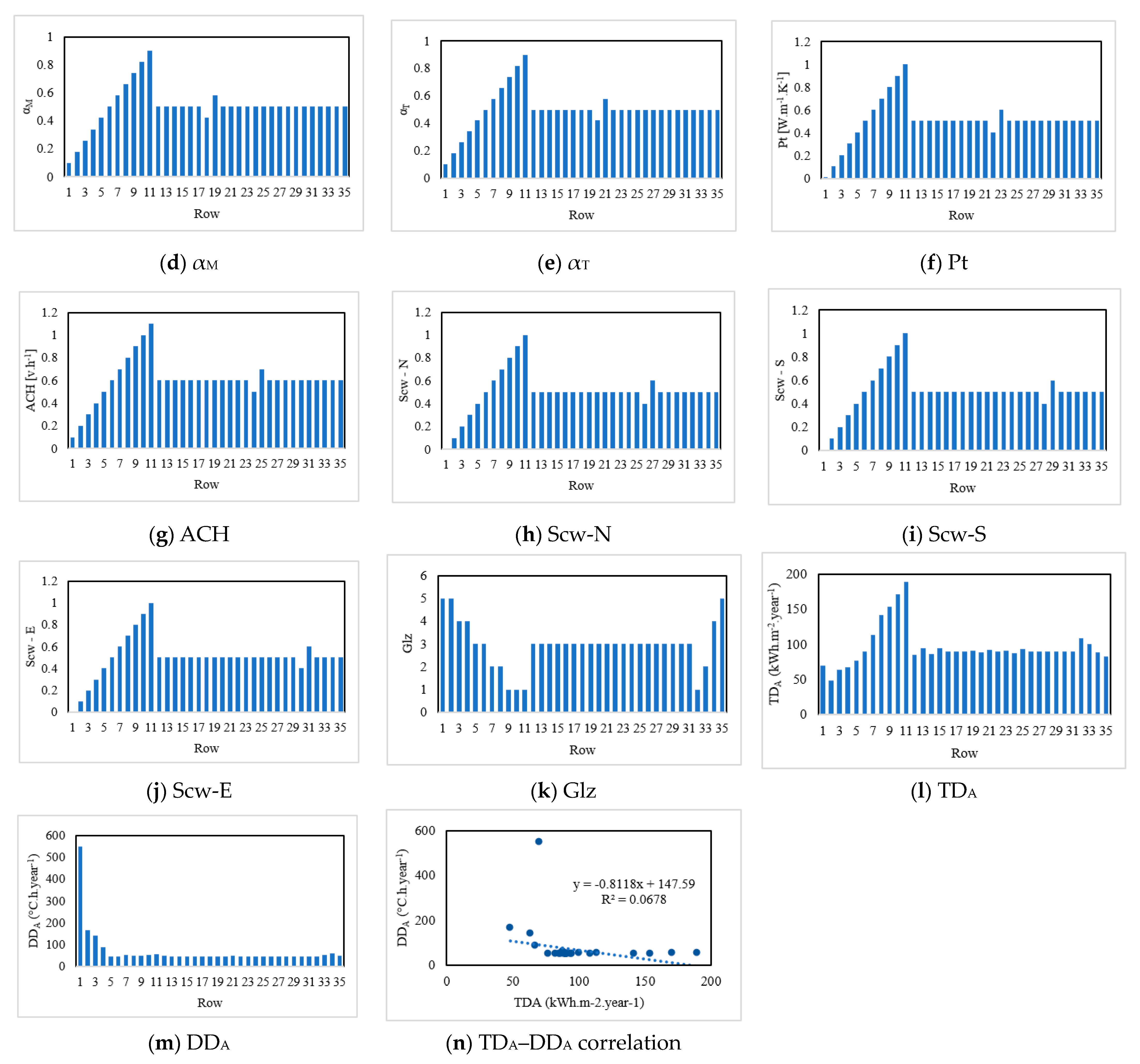
Figure 1a–k show the values of each input parameter in the form of column charts. According to these charts, except Glz, all other factors had a similar behavior, i.e., increasing values at first and then almost constant. Figure 1l,m depict the values of the target parameters TDA and DDA, respectively. Moreover, the relationship between these two parameters is presented in Figure 1n. It can be seen from these three charts that the trends of TDA and DDA did not follow a meaningful correlation, and the TDA was more compatible with the input trends.

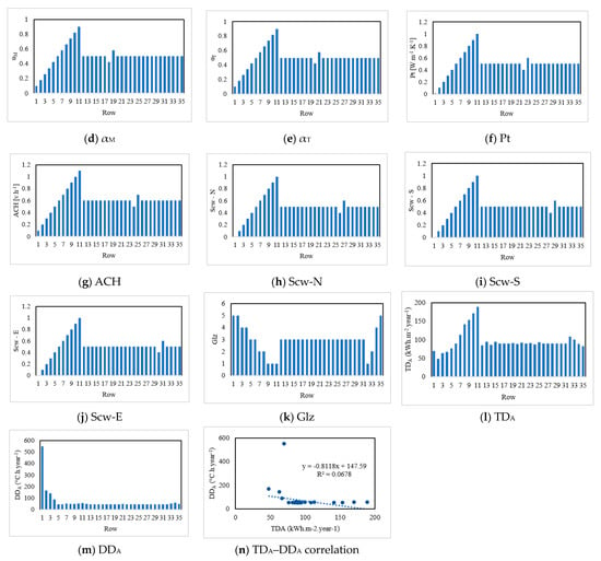
Figure 1.
Illustrating the parameters of the dataset used.
The explicit records of the 35 samples used here can be found as the supplementary material of the reference paper [33]. Table 1 presents the correlation between the input parameters with TDA and DDA. These values confirm the earlier analysis as the correlation values corresponding to TDA were much larger and indicate a direct proportionality, while those corresponding to DDA were around 30% lower and indicate an adverse proportionality for UM, UT, UP, αM, αT, Pt, ACH, Scw-N, Scw-S, and Scw-E. Not surprisingly, the behavior of Glz was in contrast to the other inputs, due to the correlation values of −0.83 and 0.47 obtained in correspondence with TDA and DDA, respectively.

Table 1.
Correlation factors showing the proportionality of the parameters.
2.2. Overview of WCA
The WCA is a potent optimization technique that is inspired by the water cycle process [35]. As is known, this process begins by raining. The raindrops are divided into three types according to their fitness values: (i) the best-fitted one is treated as the sea, (ii) a number of others with good fitness values are considered as rivers, and (iii) the remaining individuals are named streams.
The optimization using the WCA can be expressed in three major stages. In the initialization, a random population is created based on the equation:
where is the number of members, and K symbolizes the number of design dimensions. In the beginning, streams are generated, and of competent individuals are chosen as rivers and the sea (only one sea exists). Consequently, the number of streams is calculated as follows:
The amount of water that is transformed to the rivers or the sea is a function of the flow magnitude. The number of streams designated to the rivers is expressed by the equation:
where f is the evaluation function of the WCA.
The second stage is dedicated to flow and exchanges. The streams are created by raindrops, and then the streams create new rivers. The rivers all flow toward the sea, which is represented by the optimal solution. Based on Equation (4), a stream discharges its water in the river along the lines that link them together:
where d is the current distance between the stream and the river, and C is a value varying in [1, 2].
Once C > 1, the streams/rivers can flow toward the rivers/sea from different directions. The positions of these individuals are updated accordingly:
In an exchange process, the position of the new stream/river (if it is more promising than the existing one) replaces the position of the river/sea.
A measure to help the WCA avoid a premature convergence is the rainfall process. It is considered as a solution to the local optima. The algorithm first checks if the stream or river is sufficiently close to the optimal solution (i.e., the sea) to perform the raining. Hence, considering eps as a very small constant, the below conditions are defined:
During the rainfall process, new streams are generated in various places bounded within the upper and lower boundaries (Ub and Lb), as follows:
The same selection process is executed to denominate new individuals [36,37].
2.3. Benchmark Strategies
Metaheuristic schemes are mostly inspired by what is happening in nature [38,39,40]. Physical phenomena, electrical changes, and the herding behavior of animals are potential subjects for designing a metaheuristic algorithm. This paper used three benchmark optimizers along with WCA, namely the SCE, HBO, and SSA. To avoid lengthening the paper, only a brief description of these models is presented, and mathematical details are referred to via references.
The SCE is a population-based optimization technique designed by Duan et al. [41] at The University of Arizona in 1993. This algorithm, basically, is a combination of a genetic algorithm, the Nelder–Mead (downhill simplex) method, complex shuffling, and controlled random search [42]. Implementation of the SCE consists of several parameters, including generating random samples over the space, ranking the solutions based on their goodness, partitioning the complexes, evolving the complexes, shuffling the complexes, and lastly, checking for the terminating measures [43]. The SCE technique is well-detailed in the previous literature [43,44].
HBO was designed by Askari et al. [45]. The basis of this algorithm is job descriptions, titles, and responsibilities of the employees within an organization. In this technique, the process begins with splitting the task among parties by taking advantage of a so-called strategy, “CHR: corporate rank hierarchy”. Subsequent phases of the HBO are interactions with the immediate boss, colleagues’ interactions, and self-contributions of the employees. Additionally, the population is updated using the roulette wheel technique [46].
The idea of the salp swarm algorithm is obtained from the foraging behavior of these animals [47]. As a member of the Salpidae family, the salps live in the oceans in groups called chains. In the SSA, each search agent represents a possible solution that can be categorized into two groups: the followers and the leader. The leaders are responsible for guiding the rest of the chain toward food sources. It is worth noting that an advantage of the SSA is that it benefits several stochastic operators, resulting in avoiding becoming permanently trapped by local minima [48].
More mathematical details about the algorithms used here can be found in earlier studies, such as [49,50] for the SCE, [51,52] for the HBO, and [53,54] for the SSA.
Similar to the WCA, the main contribution of the SCE, HBO, and SSA lies in optimizing the 2TMLP for predicting the intended energy parameters [55]. In this process, when each algorithm is synthesized with 2TMLP, it is responsible for optimizing the 2TMLP internal variables (i.e., weights and biases) that non-linearly connect both TDA and DDA to the input factors (i.e., UM, UT, UP, αM, αT, Pt, ACH, Scw-N, Scw-S, Scw-E, and Glz). The optimization process will be explained in detail in the following sections.
2.4. Data Division
Dividing the dataset into two groups is a common task in machine learning studies [56,57]. Here, one group was introduced into the model for mathematically exploring the patterns of the TDA and DDA with reference to the behavior of the input parameters. Since these data are dedicated to training the models, they compose the major portion of the dataset. For this study, out of the 35 samples, 28 samples were used as the training data. The second group was used afterward for evaluating the goodness of the acquired knowledge when it is applied to new conditions. These are called testing data, and here contained the remaining seven samples. Note that in this step, a random division was considered to allow the training and testing datasets to have samples from throughout the original dataset.
2.5. Goodness-of-Fit Equations
The judgement of robustness of the predictive models requires exact accuracy calculations reflected by a number of statistical indices. This section introduces the accuracy criteria used for evaluating the goodness-of-fit for the results of each model. Equations (9) and (10) define two broadly used error representatives, namely root mean square error (RMSE) and mean absolute error (MAE). The RMSE is calculated by: (i) finding the difference between the real and predicted target values (i.e., and , respectively) for each pair, (ii) squaring this error, (iii) averaging the values for the whole dataset (S samples), and (iv) taking the square root of the averaged value. As for MAE, it simply calculates the error and averages it for the whole dataset.
The Pearson correlation coefficient (CR) is the third accuracy criterion which represents the percentage agreement between reality and the network predictions. According to Equation (11), the CR describes the ratio between the covariance and the standard deviations calculated for real and predicted values. The CR value of 0% means no agreement and 100% corresponds to an ideal prediction.
3. Results and Discussion
This work evaluates the proficiency of several metaheuristic algorithms that hybridize a 2TMLP for energy performance prediction in residential buildings. To present the results, this section is divided into several parts, as follows.
3.1. Hybrid Creation
Generally, to create a hybrid of the neural network and the metaheuristic technique, the training algorithm of the ANN should be replaced with the metaheuristic algorithm. The outcomes are hybrid models named SCE-2TMLP, HBO-2TMLP, SSA-2TMLP, and WCA-2TMLP. The architecture of the hybrid model (i.e., the number of variables) depends on the 2TMLP. In this work, the structure of this network was (11, 9, 2), representing 11 neurons in the input layer, 9 neurons in the middle layer, and 2 neurons in the output layer. The calculations were as follows: (i) the 11 neurons in the layer received the values of UM, UT, UP, αM, αT, Pt, ACH, Scw-N, Scw-S, Scw-E, and Glz, (ii) using 11 × 9 = 99 weights and 9 biases, the neurons in the middle layer performed the first level of calculations and sent the results to the output layer, and (iii) using 9 × 2 = 18 weights and 2 biases, the neurons in the output layer calculated the TDA and DDA.
Next, the equations governing these calculations in the 2TMLP were expressed as the problem function of the SCE, HBO, SSA, and WCA. Thus, each algorithm attempts to iteratively optimize the problem so that it attains an optimal training for the 2TMLP.
3.2. Training 2TMLP Using the Metaheuristic Algorithm
As explained, training using the metaheuristic algorithm is iterative. The number of iterations is determined based on the behavior of the algorithm. This study considered 1000 iterations for all 4 models. During each iteration of the optimization, the metaheuristic algorithm explored the training data and tuned the mentioned 128 weights and biases accordingly. The 2TMLP was then reconstructed using the tuned weights and biases and performed one prediction for all training data. To investigate the quality of the results, a cost function was required in this step. The RMSE was calculated for each iteration. Since a double-target network was being trained here, an average of the RMSEs calculated for TDA and DDA was considered as the cost function.
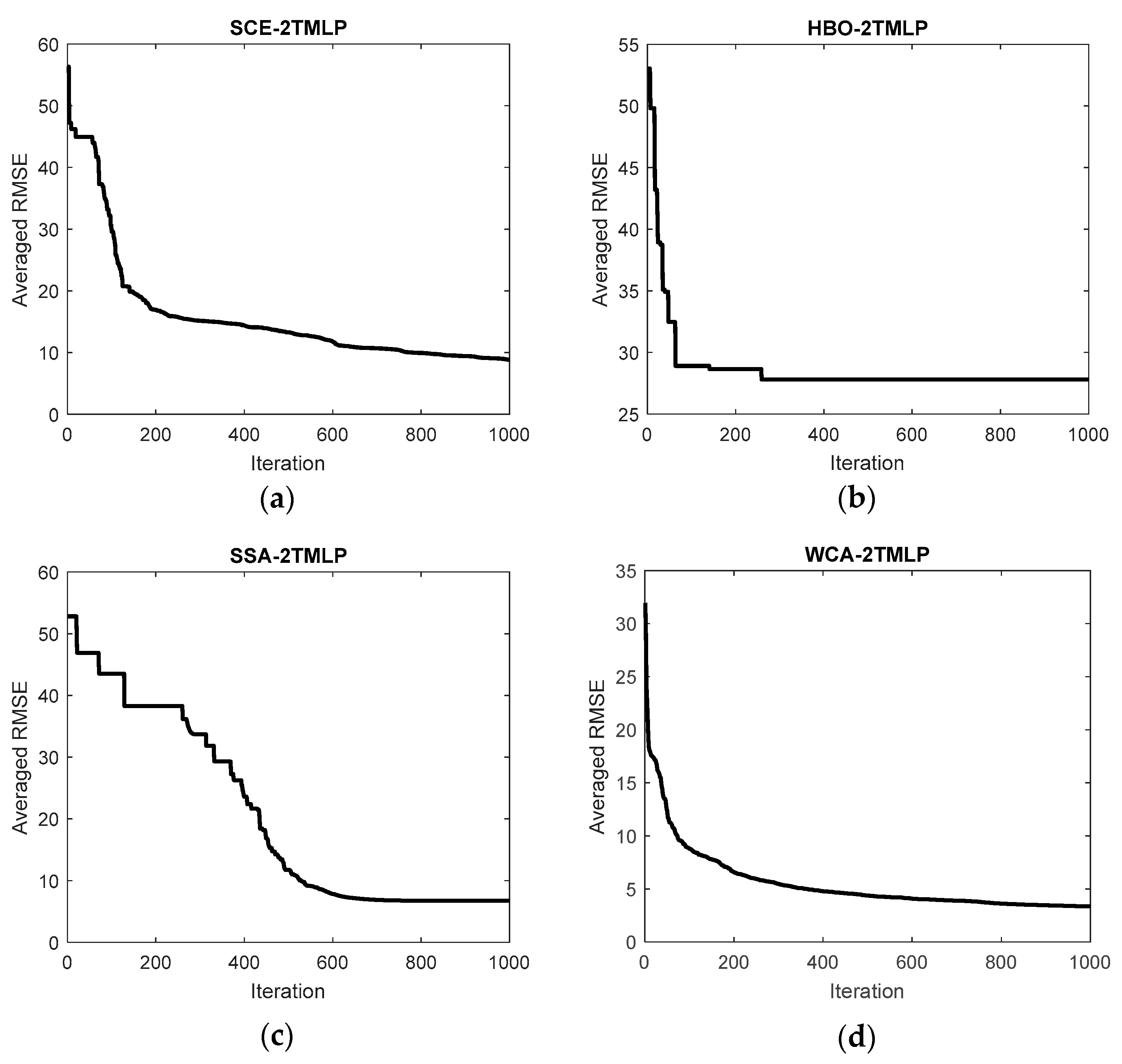
Figure 2 shows the rate of training, wherein the RMSE was generally reduced over 1000 iterations. It means that the metaheuristic algorithms were able to improve the initial solution. The behavior of all four algorithms was comparable as they reduced the RMSE quite differently from each other.
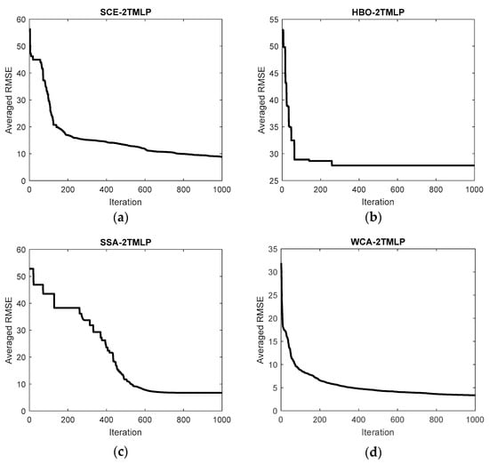
Figure 2.
Averaged cost functions obtained for optimizing 2TMLP using (a) SCE, (b) HBO, (c) SSA, and (d) WCA.
Table 2 expresses the initial and final values of the cost function obtained for each model. It can be seen that all algorithms significantly reduced the error of training. The SCE, HBO, and SSA started with a value between 50 and 60, while the initial value of WCA was around 32. Considering the final values, the SCE, SSA, and WCA ended up between 0 and 10, while this value was nearly 28 for the HBO. The lowest optimization error was eventually captured by the WCA algorithm, which was approximately 3.36.

Table 2.
Initial and final values of the cost function for each model.
3.3. Training Assessment
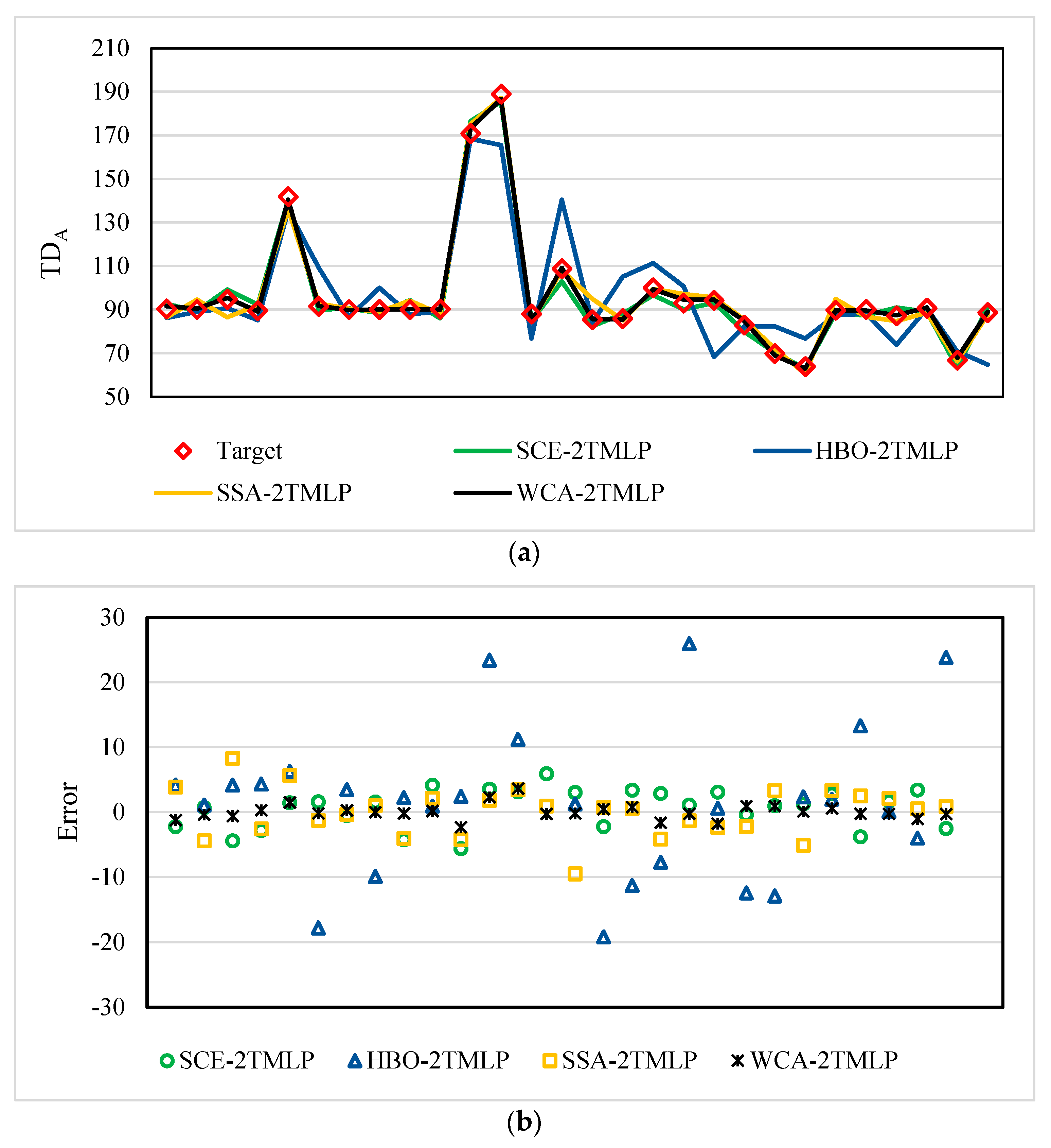
Figure 3a illustrates the training results for the TDA. This chart shows how the target values were hit by the predictions of the four models. The graphical interpretations indicated a satisfying goodness-of-fit for all models as the general patterns (i.e., significant ups and downs) were well-followed. However, a noticeable distinction could be seen between the HBO-2TMLP and the three other models. There were some overestimations and underestimations by the line of HBO-2TMLP that were more accurately modeled by SCE-2TMLP, SSA-2TMLP, and WCA-2TMLP.
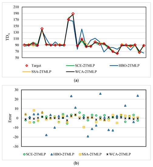
Figure 3.
Training results of TDA: (a) pattern comparison and (b) error scatter chart.
Figure 3b shows the distribution of errors in the form of a scatter chart. This chart also confirmed the lower accuracy of HBO-2TMLP as its points were more scattered compared to the other three models.
The RMSE values calculated for the SCE-2TMLP, HBO-2TMLP, SSA-2TMLP, and WCA-2TMLP were 2.66, 9.28, 2.94, and 0.81, respectively. In addition, the MAEs were 3.01, 12.71, 3.68, and 1.17. These error results, along with the CRs of 99.40%, 88.43%, 99.05%, and 99.90%, indicate a reliable prediction for all models and show the superiority of the WCA-2TMLP.
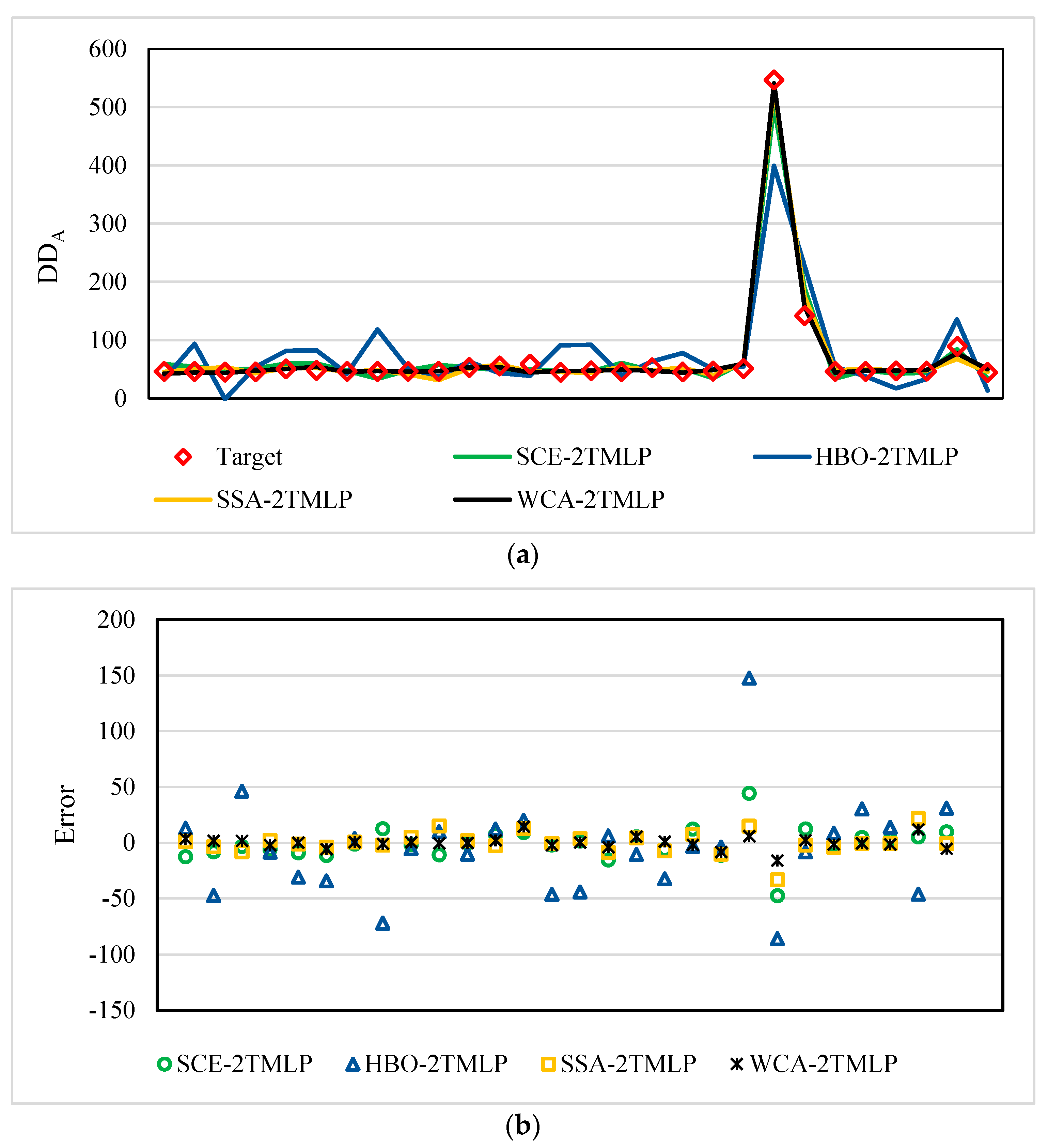
Figure 4a illustrates the training results for the DDA. The prediction results were quite promising because both small and large fluctuations were nicely recognized and followed by all models. However, similar to the DDA results, there were some weaknesses that were more tangible for the HBO-2TMLP relative to the other algorithms.
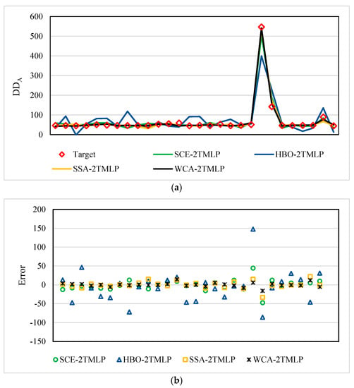
Figure 4.
Training results of DDA: (a) pattern comparison and (b) error scatter chart.
Figure 4b supports the aforementioned claims, owing to the tolerable rate of the scattered errors. Likewise, the points corresponding to HBO-2TMLP were less gathered around the ideal line, i.e., error = 0.
The RMSE values calculated for the SCE-2TMLP, HBO-2TMLP, SSA-2TMLP, and WCA-2TMLP were 14.65, 42.89, 9.77, and 5.54, respectively. In addition, the MAEs were 9.84, 29.69, 6.42, and 3.63. These error results, along with the CRs of 98.92%, 89.45%, 99.45%, and 99.82%, indicate a reliable prediction for all models and show the superiority of the WCA-2TMLP.
3.4. Testing Assessment
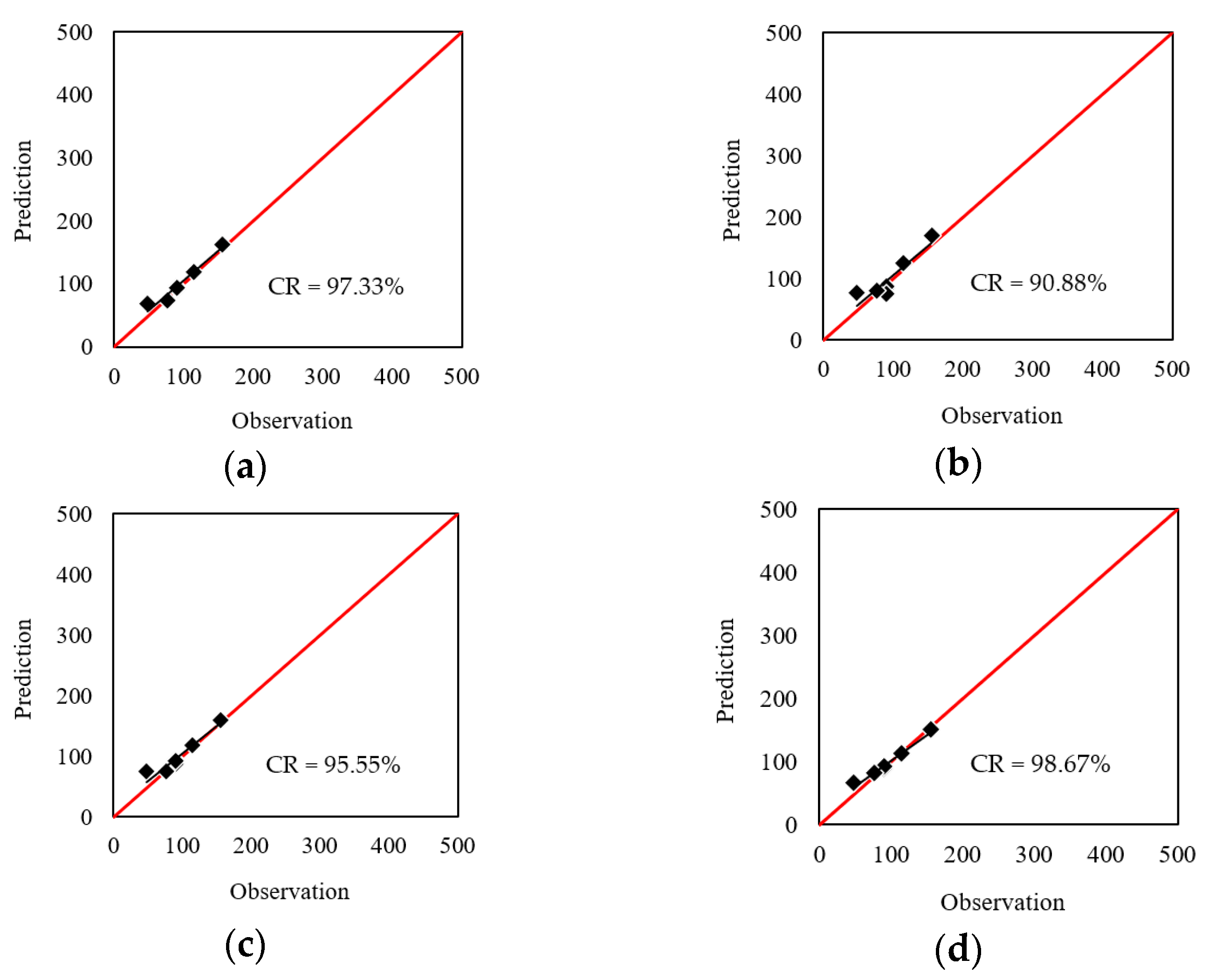
The results of the testing phase were similarly evaluated. According to the obtained RMSEs of 9.14, 14.66, 10.51, and 7.39, as well as the MAEs of 6.83, 11.70, 7.17, and 4.12, it can be deduced that all models could predict the TDA with excellent accuracy. Figure 5 shows the correlation between the real and predicted TDA values. The CR values demonstrated 97.33%, 90.88%, 95.55%, and 98.67% agreement for the results. However, similar to the previous phase, the WCA-2TMLP achieved the most accurate results in this step.
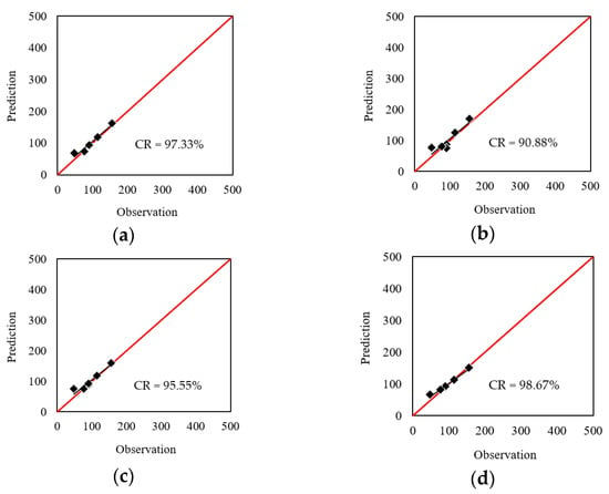
Figure 5.
Correlation of the TDA testing results obtained for: (a) SCE-2TMLP, (b) HBO-2TMLP, (c) SSA-2TMLP, and (d) WCA-2TMLP.
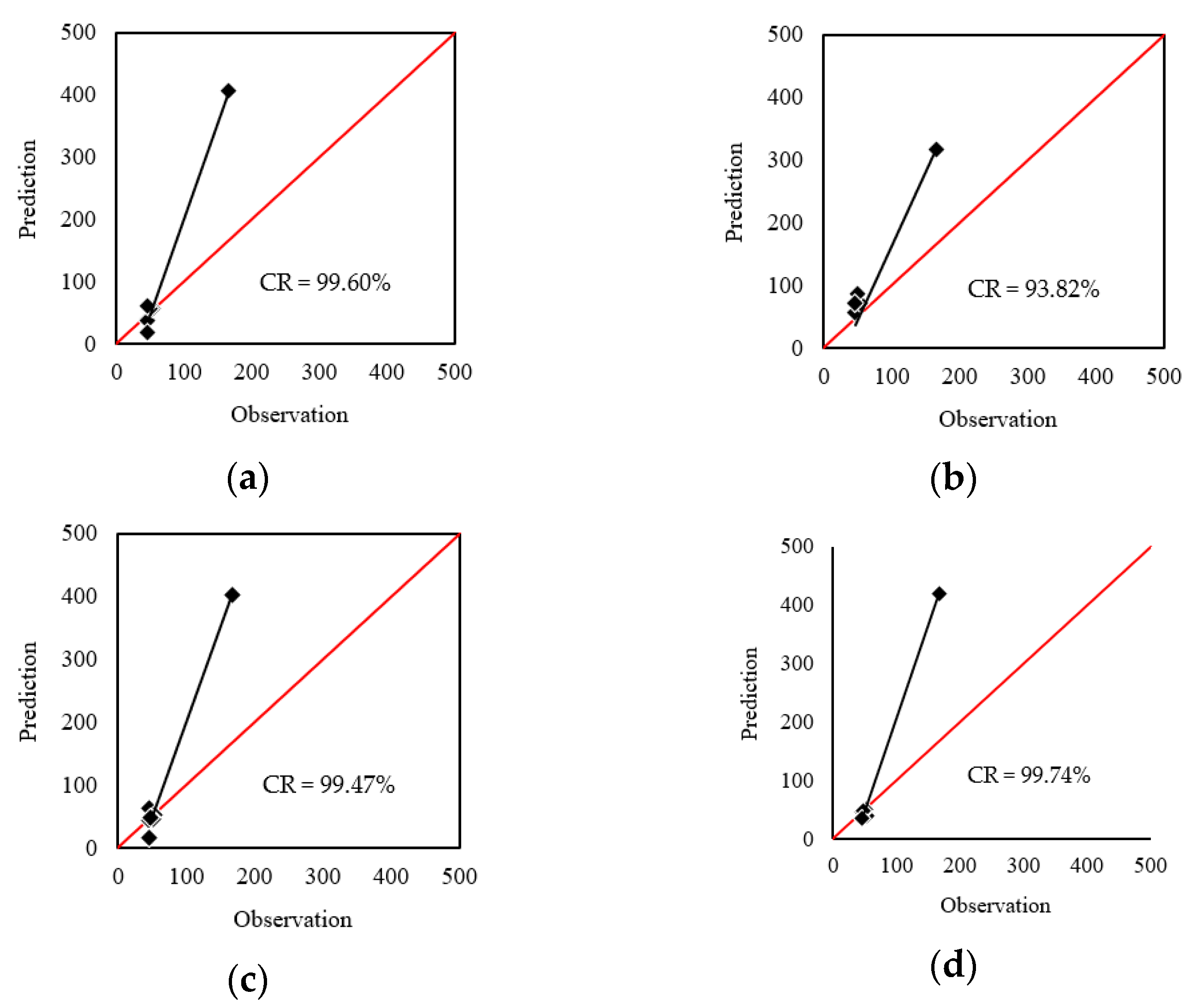
As for the DDA, the RMSE values were 91.52, 68.74, 90.15, and 96.10, associated with the MAEs of 44.01, 51.89, 41.25, and 40.07. The correlations of the DDA testing results are shown in Figure 6. Referring to the CR values of 99.60%, 93.82%, 99.47%, and 99.74%, the products of all models were in good harmony with the real values. In this phase, the WCA-2TMLP, despite achieving the smallest MAE and the largest CR, obtained the largest RMSE. However, based on the better performance in terms of two indices (out of three), the superiority of the WCA-2TMLP was evident here, too.
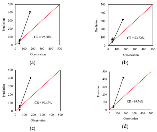
Figure 6.
Correlation of the DDA testing results obtained for: (a) SCE-2TMLP, (b) HBO-2TMLP, (c) SSA-2TMLP, and (d) WCA-2TMLP.
3.5. Comparison
Table 3, Table 4 and Table 5 present the values of the RMSE, MAE, and CR, respectively, calculated for training and testing both the TDA and DDA. From the overall comparison, it was found that the WCA-2TMLP had the largest accuracy in most stages. More clearly, for the TDA analysis (in both phases), the order of the algorithms from strongest to weakest was: (1) WCA-2TMLP, (2) SCE-2TMLP, (3) SSA-2TMLP, and (4) HBO-2TMLP. However, the outcome was different for the DDA analysis. While the training RMSE demonstrated the lowest error for WCA-2TMLP and the highest for HBO-2TMLP, the ranking was adverse in the testing phase. In both phases, the SSA-2TMLP captured the second position, followed by SCE-2TMLP. However, the MAE consistently suggested the following ranking: (1) WCA-2TMLP, (2) SSA-2TMLP, (3) SCE-2TMLP, and (4) HBO-2TMLP. As for the CR, the WCA-2TMLP and HBO-2TMLP were the strongest and the weakest predictor in both phases, respectively, while the SSA-2TMLP and SCE-2TMLP shared the second and third positions interchangeably in the training and testing phases.

Table 3.
The results of the RMSE calculation.

Table 4.
The results of the MAE calculation.

Table 5.
The results of the CR calculation.
In summary, in terms of accuracy, the WCA was introduced as the most effective metaheuristic algorithm in this study. The SSA and SCE provided reliable solutions and are recommended for practical applications as well, and the results of HBO do not make it preferable. Considering the time of optimization, the implementation of SCE, HBO, SSA, and WCA required about 782, 79,717, 8507, and 60,281 s. Hence, utilizing the WCA was more time-consuming relative to the SSA and the SCE. Due to the sufficient accuracy of the SCE, as well as the shortest time of optimization achieved, it can be suitable for time-sensitive cases, along with WCA.
3.6. Discussion
Studying the buildings comprises a wide range of domains, from safety measures [58] and external designs [59] to structural [60] and energy performance analysis [61]. Recently, the development of smart cities has affected construction- and energy-related policies in the construction sector [62,63]. Following the previous efforts of energy engineers in forecasting energy performance of residential building using intelligent approaches, this work presented novel ANN-based models for this purpose.
Referring to the literature, it was pointed out that the combination of ANN and WCA has provided optimized solutions for various intricate engineering simulations, such as spatial analysis of environmental phenomena (e.g., groundwater potential [64]). This algorithm has also provided effective solutions for energy simulations (e.g., electrical power output of power plants [31]). In comparative studies, a reason for the superiority of the WCA has been its muti-directional optimization strategy, as well as its multi-rain process that protects the solution against local minima [37].
In the application of metaheuristic algorithms, population size is one of the most prominent hyperparameters. In this work, the selection of population size for all algorithms was performed by trial-and-error. The population sizes used were 10, 50, 100, 200, 300, 400, and 500. It was discovered that 10, 300, 400, and 500 fit the best for the SCE, HBO, SSA, and WCA, respectively.
Earlier literature demonstrates that the findings of this research are in harmony with previous studies that have addressed the applicability of metaheuristic techniques in the field of energy performance analysis. In a broad comparative study by Lin and Wang [32], the evident superiority of the WCA was reported for predicting the heating and cooling loads of residential buildings using a public dataset provided by Tsanas and Xifara [65]. The benchmark algorithms were the equilibrium optimizer (EO), the multi-verse optimizer (MVO), the multi-tracker optimization algorithm (MTOA), electromagnetic field optimization (EFO), and the slime mold algorithm (SMA). Concerning the present dataset, the methodology offered in this work outperformed some previous models. For instance, in adaptive neuro-fuzzy inference system (ANFIS) optimization, carried out by Alkhazaleh et al. [66] for the TDA prediction using EO and Harris hawks optimization (HHO), the best model was ANFIS-400-EO, which achieved a training MAE = 1.87, while in this work the lowest MAE was 0.81. As for testing, the lowest MAE of the cited study was 5.74, obtained by ANFIS-100-HHO, while this study reduced it to 4.12 using WCA-2TMLP. Hence, significant improvements can be detected.
The size of the dataset used in this study was relatively small (i.e., 35 samples). However, referring to the results, it was shown that the models were able to obtain a very reliable understanding of the building energy behavior using 28 samples, and they could accurately extrapolate the knowledge to the remaining 7 samples. This dataset has also been reported to be suitable for developing metaheuristic-based hybrids in similar previous studies [66,67]. However, it would be interesting for the future studies to investigate the sensitivity of prediction accuracy on the size of the dataset. Creating similar datasets is highly suggested to cross-validate the methodologies presented so far.
The dataset used here was bounded to taking 11 influential parameters into account. Hence, another noticeable suggestion about the dataset could be extending the dataset through considering further building characteristics and design parameters that can directly/indirectly affect the energy performance (e.g., window-to-wall ratio, U-value of walls/windows, unplanned air exchange between the building and environment, etc.). Once provided, the dataset may be subjected to a feature selection process in order to maintain the most contributive parameters and discard the negligible ones. In doing so, not only would a more realistic assessment be achieved, but also the methodology would be optimized by reducing the dimensions of the problem.
3.7. TDA and DDA Formula
With reference to the suitable results presented by the SCE-2TMLP, the governing equations organized by the SCE algorithm are provided as a predictive formula for simultaneous estimation of the TDA and DDA. Based on the architecture of the 2TMLP (i.e., 11 input neurons, 9 hidden neurons with Tansig activation, and 2 output neurons with Purelin activation function), the procedure of calculating the TDA and DDA requires producing 9 outputs from the middle layer. As expressed by Equations (12) and (13), as well as Table 6, each of these outputs (represented by O1, O2, …, O9) is a non-linear function of the input parameters (i.e., UM, UT, UP, αM, αT, Pt, ACH, Scw-N, Scw-S, Scw-E, and Glz).
where,
from which, the weights, Wi1, Wi2, …, Wi11, as well as the biases, bi, are presented in Table 3.

Table 6.
The solution (weights and biases) of the 2TMLP.
Once O1, O2, …, O9 are calculated, Equations (14) and (15) yield the TDA and DDA, respectively. The reason for the linear calculations in these two equations lies in the Purelin function, which is described as f(x) = x.
TDA = −0.198 × O1 − 0.874 × O2 + 0.940 × O3 + 0.315 × O4 + 0.422 × O5 + 0.666 × O6 − 0.307 × O7 − 0.517 × O8 − 0.852 × O9 − 0.193,
DDA = 0.961 × O1 − 0.979 × O2 − 0.964 × O3 − 0.523 × O4 − 0.644 × O5 + 0.862 × O6 + 0.612 × O7 + 0.370 × O8 + 0.051 × O9 + 0.638
4. Conclusions
Based on the previous recommendations regarding the use of intelligent models for energy performance assessments, this study was dedicated to introducing and evaluating a new methodology based on artificial intelligence for energy performance analysis in residential buildings. The water cycle algorithm effectively enabled a double-target MLP neural network to predict the annual thermal energy demand and annual weighted average discomfort degree-hours in residential buildings. It was the first finding that reflected the competency of metaheuristic–neural configurations for this purpose. Based on the accuracy evaluations reported from RMSE, MAE, and CR indices, the proposed WCA model could not only fulfill the task with great accuracy, but it also performed more accurately in comparison with shuffled complex evolution, the heap-based optimizer, and the salp swarm algorithm. The findings of this work asserted the suitability of metaheuristic algorithms for attaining optimal weights and biases for the 2TMLP, and thereby, for handling the simultaneous estimation of energy-related parameters by analyzing the geometry and architecture of the building. From a practical aspect, the outcomes are interesting to energy management experts working on sustainable development of smart buildings. This work also provided some suggestions for future efforts for improving the data usage and strategies.
Author Contributions
Investigation, C.L. and Y.L.; Supervision, C.L. All authors have read and agreed to the published version of the manuscript.
Funding
This work was supported by the postgraduate innovation special fund project of Jiangxi Province (YC2022-s476).
Data Availability Statement
The data used in this article are available as explained in Section 2.1.
Conflicts of Interest
The authors declare no conflict of interest.
Nomenclature
| ANN | Artificial neural network |
| ANFIS | Adaptive neuro-fuzzy inference system |
| WCA | Water cycle algorithm |
| 2TMLP | Double-target multi-layer perceptron |
| SCE | Shuffled complex evolution |
| EFA | Electromagnetism-based firefly algorithm |
| MR | Multiple regression |
| GP | Genetic programming |
| DNN | Deep neural network |
| SVM | Support vector machine |
| SVR | Support vector regression |
| GB | Gradient boosting |
| KNN | K-nearest neighbor |
| DT | Decision tree |
| XGBoost | Extreme gradient boosting |
| DELM | Deep extreme learning |
| LSTM | Long short-term memory |
| KF | Kalman filter |
| DCNN | Convolutional neural network |
| BiLSTM | Bidirectional long short-term memory |
| GRU | Gated recurrent unit |
| BIM | Building information modeling |
| HBO | Heap-based optimizer |
| SSA | Salp swarm algorithm |
| EO | Equilibrium optimizer |
| MVO | Multi-verse optimizer |
| MTOA | Multi-tracker optimization algorithm |
| EFO | Electromagnetic field optimization |
| SMA | Slime mold algorithm |
| HHO | Harris hawks optimization |
| UM | Transmission coefficient of the external walls |
| UT | Transmission coefficient of the roof |
| UP | Transmission coefficient of the floor |
| αM | Solar radiation absorption coefficient of the exterior walls |
| αT | Solar radiation absorption coefficient of the roof |
| Pt | Linear coefficient of thermal bridges |
| ACH | Air change rate |
| Scw-N | Shading coefficient of north-facing windows |
| Scw-S | Shading coefficient of south-facing windows |
| Scw-E | Shading coefficient of east-facing windows |
| Glz | Glazing |
| MAE | Mean absolute error |
| RMSE | Root mean square error |
| CR | Pearson correlation index |
| DDA | Weighted average discomfort degree-hours |
| TDA | Thermal energy demand |
References
- Tri, N.M.; Hoang, P.D.; Dung, N.T. Impact of the industrial revolution 4.0 on higher education in Vietnam: Challenges and opportunities. Linguist. Cult. Rev. 2021, 5, 1–15. [Google Scholar] [CrossRef]
- Khan, A.; Aslam, S.; Aurangzeb, K.; Alhussein, M.; Javaid, N. Multiscale modeling in smart cities: A survey on applications, current trends, and challenges. Sustain. Cities Soc. 2022, 78, 103517. [Google Scholar] [CrossRef]
- Singh, T.; Solanki, A.; Sharma, S.K.; Nayyar, A.; Paul, A. A Decade Review on Smart Cities: Paradigms, Challenges and Opportunities. IEEE Access 2022, 10, 68319–68364. [Google Scholar] [CrossRef]
- Nejat, P.; Jomehzadeh, F.; Taheri, M.M.; Gohari, M.; Abd Majid, M.Z. A global review of energy consumption, CO2 emissions and policy in the residential sector (with an overview of the top ten CO2 emitting countries). Renew. Sustain. Energy Rev. 2015, 43, 843–862. [Google Scholar] [CrossRef]
- Abdelkader, E.; Al-Sakkaf, A.; Ahmed, R. A comprehensive comparative analysis of machine learning models for predicting heating and cooling loads. Decis. Sci. Lett. 2020, 9, 409–420. [Google Scholar] [CrossRef]
- Kim, T.-Y.; Cho, S.-B. Predicting residential energy consumption using CNN-LSTM neural networks. Energy 2019, 182, 72–81. [Google Scholar] [CrossRef]
- Wei, N.; Li, C.; Peng, X.; Zeng, F.; Lu, X. Conventional models and artificial intelligence-based models for energy consumption forecasting: A review. J. Pet. Sci. Eng. 2019, 181, 106187. [Google Scholar] [CrossRef]
- Meng, S.; Wang, X.; Hu, X.; Luo, C.; Zhong, Y. Deep learning-based crop mapping in the cloudy season using one-shot hyperspectral satellite imagery. Comput. Electron. Agric. 2021, 186, 106188. [Google Scholar] [CrossRef]
- Bui, D.-K.; Nguyen, T.N.; Ngo, T.D.; Nguyen-Xuan, H. An artificial neural network (ANN) expert system enhanced with the electromagnetism-based firefly algorithm (EFA) for predicting the energy consumption in buildings. Energy 2020, 190, 116370. [Google Scholar] [CrossRef]
- Amber, K.P.; Ahmad, R.; Aslam, M.W.; Kousar, A.; Usman, M.; Khan, M.S. Intelligent techniques for forecasting electricity consumption of buildings. Energy 2018, 157, 886–893. [Google Scholar] [CrossRef]
- Ma, Z.; Ye, C.; Li, H.; Ma, W. Applying support vector machines to predict building energy consumption in China. Energy Procedia 2018, 152, 780–786. [Google Scholar] [CrossRef]
- Zhang, X.M.; Grolinger, K.; Capretz, M.A.M.; Seewald, L. Forecasting Residential Energy Consumption: Single Household Perspective. In Proceedings of the 2018 17th IEEE International Conference on Machine Learning and Applications (ICMLA), Orlando, FL, USA, 17–20 December 2018; pp. 110–117. [Google Scholar]
- Olu-Ajayi, R.; Alaka, H.; Sulaimon, I.; Sunmola, F.; Ajayi, S. Building energy consumption prediction for residential buildings using deep learning and other machine learning techniques. J. Build. Eng. 2022, 45, 103406. [Google Scholar] [CrossRef]
- Banik, R.; Das, P.; Ray, S.; Biswas, A. Prediction of electrical energy consumption based on machine learning technique. Electr. Eng. 2021, 103, 909–920. [Google Scholar] [CrossRef]
- Gao, W.; Alsarraf, J.; Moayedi, H.; Shahsavar, A.; Nguyen, H. Comprehensive preference learning and feature validity for designing energy-efficient residential buildings using machine learning paradigms. Appl. Soft Comput. 2019, 84, 105748. [Google Scholar] [CrossRef]
- Moayedi, H.; Ghareh, S.; Foong, L.K. Quick integrative optimizers for minimizing the error of neural computing in pan evaporation modeling. Eng. Comput. 2021, 38, 1331–1347. [Google Scholar] [CrossRef]
- Mehrabi, M. Landslide susceptibility zonation using statistical and machine learning approaches in Northern Lecco, Italy. Nat. Hazards 2021, 111, 901–937. [Google Scholar] [CrossRef]
- Fayaz, M.; Kim, D. A Prediction Methodology of Energy Consumption Based on Deep Extreme Learning Machine and Comparative Analysis in Residential Buildings. Electronics 2018, 7, 222. [Google Scholar] [CrossRef]
- Khan, A.N.; Iqbal, N.; Ahmad, R.; Kim, D.-H. Ensemble Prediction Approach Based on Learning to Statistical Model for Efficient Building Energy Consumption Management. Symmetry 2021, 13, 405. [Google Scholar] [CrossRef]
- Li, Y.; Tong, Z.; Tong, S.; Westerdahl, D. A data-driven interval forecasting model for building energy prediction using attention-based LSTM and fuzzy information granulation. Sustain. Cities Soc. 2022, 76, 103481. [Google Scholar] [CrossRef]
- Khan, N.; Haq, I.U.; Khan, S.U.; Rho, S.; Lee, M.Y.; Baik, S.W. DB-Net: A novel dilated CNN based multi-step forecasting model for power consumption in integrated local energy systems. Int. J. Electr. Power Energy Syst. 2021, 133, 107023. [Google Scholar] [CrossRef]
- Khan, A.-N.; Iqbal, N.; Rizwan, A.; Ahmad, R.; Kim, D.-H. An Ensemble Energy Consumption Forecasting Model Based on Spatial-Temporal Clustering Analysis in Residential Buildings. Energies 2021, 14, 3020. [Google Scholar] [CrossRef]
- Chen, B.; Liu, Q.; Chen, H.; Wang, L.; Deng, T.; Zhang, L.; Wu, X. Multiobjective optimization of building energy consumption based on BIM-DB and LSSVM-NSGA-II. J. Clean. Prod. 2021, 294, 126153. [Google Scholar] [CrossRef]
- Moon, J.; Park, S.; Rho, S.; Hwang, E. Robust building energy consumption forecasting using an online learning approach with R ranger. J. Build. Eng. 2022, 47, 103851. [Google Scholar] [CrossRef]
- Phyo, P.-P.; Jeenanunta, C. Advanced ML-Based Ensemble and Deep Learning Models for Short-Term Load Forecasting: Comparative Analysis Using Feature Engineering. Appl. Sci. 2022, 12, 4882. [Google Scholar] [CrossRef]
- Li, X.; Sun, Y. Stock intelligent investment strategy based on support vector machine parameter optimization algorithm. Neural Comput. Appl. 2020, 32, 1765–1775. [Google Scholar] [CrossRef]
- Mehrabi, M.; Pradhan, B.; Moayedi, H.; Alamri, A. Optimizing an adaptive neuro-fuzzy inference system for spatial prediction of landslide susceptibility using four state-of-the-art metaheuristic techniques. Sensors 2020, 20, 1723. [Google Scholar] [CrossRef]
- Almutairi, K.; Algarni, S.; Alqahtani, T.; Moayedi, H.; Mosavi, A. A TLBO-Tuned Neural Processor for Predicting Heating Load in Residential Buildings. Sustainability 2022, 14, 5924. [Google Scholar] [CrossRef]
- Moayedi, H.; Mosavi, A. Synthesizing multi-layer perceptron network with ant lion biogeography-based dragonfly algorithm evolutionary strategy invasive weed and league champion optimization hybrid algorithms in predicting heating load in residential buildings. Sustainability 2021, 13, 3198. [Google Scholar] [CrossRef]
- Foong, L.K.; Moayedi, H.; Lyu, Z. Computational modification of neural systems using a novel stochastic search scheme, namely evaporation rate-based water cycle algorithm: An application in geotechnical issues. Eng. Comput. 2021, 37, 3347–3358. [Google Scholar] [CrossRef]
- Moayedi, H.; Mosavi, A. Electrical power prediction through a combination of multilayer perceptron with water cycle ant lion and satin bowerbird searching optimizers. Sustainability 2021, 13, 2336. [Google Scholar] [CrossRef]
- Lin, C.; Wang, J. Metaheuristic-designed systems for simultaneous simulation of thermal loads of building. Smart Struct. Syst. 2022, 29, 677–691. [Google Scholar]
- Chegari, B.; Tabaa, M.; Simeu, E.; Moutaouakkil, F.; Medromi, H. Multi-objective optimization of building energy performance and indoor thermal comfort by combining artificial neural networks and metaheuristic algorithms. Energy Build. 2021, 239, 110839. [Google Scholar] [CrossRef]
- Klein, S.; Beckman, W.; Mitchell, J.; Duffie, J.; Duffie, N.; Freeman, T.; Mitchell, J.; Braun, J.; Evans, B.; Kummer, J. TRNSYS 17: A Transient System Simulation Program, Solar Energy Laboratory; University of Wisconsin: Madison, WI, USA, 2010. [Google Scholar]
- Eskandar, H.; Sadollah, A.; Bahreininejad, A.; Hamdi, M. Water cycle algorithm—A novel metaheuristic optimization method for solving constrained engineering optimization problems. Comput. Struct. 2012, 110, 151–166. [Google Scholar] [CrossRef]
- Luo, Q.; Wen, C.; Qiao, S.; Zhou, Y. Dual-system water cycle algorithm for constrained engineering optimization problems. In Proceedings of the International Conference on Intelligent Computing, Lanzhou, China, 2–5 August 2016; Springer: Berlin/Heidelberg, Germany, 2016; pp. 730–741. [Google Scholar]
- Mehrabi, M.; Moayedi, H. Landslide susceptibility mapping using artificial neural network tuned by metaheuristic algorithms. Environ. Earth Sci. 2021, 80, 804. [Google Scholar] [CrossRef]
- Caraveo, C.; Valdez, F.; Castillo, O. A new optimization meta-heuristic algorithm based on self-defense mechanism of the plants with three reproduction operators. Soft Comput. 2018, 22, 4907–4920. [Google Scholar] [CrossRef]
- Olivas, F.; Valdez, F.; Melin, P.; Sombra, A.; Castillo, O. Interval type-2 fuzzy logic for dynamic parameter adaptation in a modified gravitational search algorithm. Inf. Sci. 2019, 476, 159–175. [Google Scholar] [CrossRef]
- Castillo, O.; Valdez, F.; Soria, J.; Amador-Angulo, L.; Ochoa, P.; Peraza, C. Comparative study in fuzzy controller optimization using bee colony, differential evolution, and harmony search algorithms. Algorithms 2019, 12, 9. [Google Scholar] [CrossRef]
- Duan, Q.; Gupta, V.K.; Sorooshian, S. Shuffled complex evolution approach for effective and efficient global minimization. J. Optim. Theory Appl. 1993, 76, 501–521. [Google Scholar] [CrossRef]
- Ira, J.; Hasalová, L.; Jahoda, M. The use of optimization in fire development modeling, The use of optimization techniques for estimation of pyrolysis model input parameters. Applications of Structural Fire Engineering. 2015. Available online: https://ojs.cvut.cz/ojs/index.php/asfe/article/view/3095 (accessed on 12 April 2023).
- Meshkat Razavi, H.; Shariatmadar, H. Optimum parameters for tuned mass damper using Shuffled Complex Evolution (SCE) Algorithm. Civ. Eng. Infrastruct. J. 2015, 48, 83–100. [Google Scholar]
- Baroni, M.D.V.; Varejão, F.M. A shuffled complex evolution algorithm for the multidimensional knapsack problem. In Proceedings of the Iberoamerican Congress on Pattern Recognition, Kuala Lumpur, Malaysia, 3–6 November 2015; Springer: Berlin/Heidelberg, Germany, 2015; pp. 768–775. [Google Scholar]
- Askari, Q.; Saeed, M.; Younas, I. Heap-based optimizer inspired by corporate rank hierarchy for global optimization. Expert Syst. Appl. 2020, 161, 113702. [Google Scholar] [CrossRef]
- AbdElminaam, D.S.; Houssein, E.H.; Said, M.; Oliva, D.; Nabil, A. An efficient heap-based optimizer for parameters identification of modified photovoltaic models. Ain Shams Eng. J. 2022, 13, 101728. [Google Scholar] [CrossRef]
- Mirjalili, S.; Gandomi, A.H.; Mirjalili, S.Z.; Saremi, S.; Faris, H.; Mirjalili, S.M. Salp Swarm Algorithm: A bio-inspired optimizer for engineering design problems. Adv. Eng. Softw. 2017, 114, 163–191. [Google Scholar] [CrossRef]
- Faris, H.; Mafarja, M.M.; Heidari, A.A.; Aljarah, I.; Ala’M, A.-Z.; Mirjalili, S.; Fujita, H. An efficient binary salp swarm algorithm with crossover scheme for feature selection problems. Knowl. Based Syst. 2018, 154, 43–67. [Google Scholar] [CrossRef]
- Zhang, J.; Sun, L.; Zhong, Y.; Ding, Y.; Du, W.; Lu, K.; Jia, J. Kinetic model and parameters optimization for Tangkou bituminous coal by the bi-Gaussian function and Shuffled Complex Evolution. Energy 2022, 243, 123012. [Google Scholar] [CrossRef]
- Zheng, S.; Lyu, Z.; Foong, L.K. Early prediction of cooling load in energy-efficient buildings through novel optimizer of shuffled complex evolution. Eng. Comput. 2020, 38, 105–119. [Google Scholar] [CrossRef]
- Shaheen, A.M.; Elsayed, A.M.; Ginidi, A.R.; El-Sehiemy, R.A.; Elattar, E.E. Improved heap-based optimizer for dg allocation in reconfigured radial feeder distribution systems. IEEE Syst. J. 2022, 16, 6371–6380. [Google Scholar] [CrossRef]
- Ewees, A.A.; Al-qaness, M.A.; Abualigah, L.; Abd Elaziz, M. HBO-LSTM: Optimized long short term memory with heap-based optimizer for wind power forecasting. Energy Convers. Manag. 2022, 268, 116022. [Google Scholar] [CrossRef]
- Gupta, S.; Deep, K.; Heidari, A.A.; Moayedi, H.; Chen, H. Harmonized salp chain-built optimization. Eng. Comput. 2019, 37, 1049–1079. [Google Scholar] [CrossRef]
- Tubishat, M.; Idris, N.; Shuib, L.; Abushariah, M.A.; Mirjalili, S. Improved Salp Swarm Algorithm based on opposition based learning and novel local search algorithm for feature selection. Expert Syst. Appl. 2020, 145, 113122. [Google Scholar] [CrossRef]
- Moayedi, H.; Mehrabi, M.; Mosallanezhad, M.; Rashid, A.S.A.; Pradhan, B. Modification of landslide susceptibility mapping using optimized PSO-ANN technique. Eng. Comput. 2018, 35, 967–984. [Google Scholar] [CrossRef]
- Moayedi, H.; Mehrabi, M.; Bui, D.T.; Pradhan, B.; Foong, L.K. Fuzzy-metaheuristic ensembles for spatial assessment of forest fire susceptibility. J. Environ. Manag. 2020, 260, 109867. [Google Scholar] [CrossRef] [PubMed]
- Moayedi, H.; Mehrabi, M.; Kalantar, B.; Abdullahi Mu’azu, M.; Rashid, A.S.A.; Foong, L.K.; Nguyen, H. Novel hybrids of adaptive neuro-fuzzy inference system (ANFIS) with several metaheuristic algorithms for spatial susceptibility assessment of seismic-induced landslide. Geomat. Nat. Hazards Risk 2019, 10, 1879–1911. [Google Scholar] [CrossRef]
- Zhang, Z.; Li, W.; Yang, J. Analysis of stochastic process to model safety risk in construction industry. J. Civ. Eng. Manag. 2021, 27, 87–99. [Google Scholar] [CrossRef]
- Zhou, G.; Bao, X.; Ye, S.; Wang, H.; Yan, H. Selection of optimal building facade texture images from UAV-based multiple oblique image flows. IEEE Trans. Geosci. Remote Sens. 2020, 59, 1534–1552. [Google Scholar] [CrossRef]
- Liu, H.; Chen, Z.; Liu, Y.; Chen, Y.; Du, Y.; Zhou, F. Interfacial debonding detection for CFST structures using an ultrasonic phased array: Application to the Shenzhen SEG building. Mech. Syst. Signal Process. 2023, 192, 110214. [Google Scholar] [CrossRef]
- Balo, F.; Ulutaş, A. Energy-Performance Evaluation with Revit Analysis of Mathematical-Model-Based Optimal Insulation Thickness. Buildings 2023, 13, 408. [Google Scholar] [CrossRef]
- Guo, Q.; Zhong, J. The effect of urban innovation performance of smart city construction policies: Evaluate by using a multiple period difference-in-differences model. Technol. Forecast. Soc. Chang. 2022, 184, 122003. [Google Scholar] [CrossRef]
- Shang, Y.; Lian, Y.; Chen, H.; Qian, F. The impacts of energy resource and tourism on green growth: Evidence from Asian economies. Resour. Policy 2023, 81, 103359. [Google Scholar] [CrossRef]
- Asadi Nalivan, O.; Mousavi Tayebi, S.A.; Mehrabi, M.; Ghasemieh, H.; Scaioni, M. A hybrid intelligent model for spatial analysis of groundwater potential around Urmia Lake, Iran. Stoch. Environ. Res. Risk Assess. 2022, 1–18. [Google Scholar] [CrossRef]
- Tsanas, A.; Xifara, A. Accurate quantitative estimation of energy performance of residential buildings using statistical machine learning tools. Energy Build. 2012, 49, 560–567. [Google Scholar] [CrossRef]
- Alkhazaleh, H.A.; Nahi, N.; Hashemian, M.H.; Nazem, Z.; Shamsi, W.D.; Nehdi, M.L. Prediction of Thermal Energy Demand Using Fuzzy-Based Models Synthesized with Metaheuristic Algorithms. Sustainability 2022, 14, 14385. [Google Scholar] [CrossRef]
- Fallah, A.M.; Ghafourian, E.; Shahzamani Sichani, L.; Ghafourian, H.; Arandian, B.; Nehdi, M.L. Novel Neural Network Optimized by Electrostatic Discharge Algorithm for Modification of Buildings Energy Performance. Sustainability 2023, 15, 2884. [Google Scholar] [CrossRef]
Disclaimer/Publisher’s Note: The statements, opinions and data contained in all publications are solely those of the individual author(s) and contributor(s) and not of MDPI and/or the editor(s). MDPI and/or the editor(s) disclaim responsibility for any injury to people or property resulting from any ideas, methods, instructions or products referred to in the content. |
© 2023 by the authors. Licensee MDPI, Basel, Switzerland. This article is an open access article distributed under the terms and conditions of the Creative Commons Attribution (CC BY) license (https://creativecommons.org/licenses/by/4.0/).


