Article

Bayesian RC-Frame Finite Element Model Updating and Damage Estimation Using Nested Sampling with Nonlinear Time History

1
Division of Structural and Earthquake Engineering, Department of Civil Engineering, Graduate School of Engineering, Kyushu University, Fukuoka 8190385, Japan
2
Department of Civil and Structural Engineering, Faculty of Engineering, Kyushu University, Fukuoka 8190385, Japan
3
YJK Building Software, Beijing 100013, China
*
Author to whom correspondence should be addressed.
Buildings 2023, 13(5), 1281; https://doi.org/10.3390/buildings13051281
Submission received: 16 March 2023 / Revised: 12 April 2023 / Accepted: 11 May 2023 / Published: 14 May 2023

Abstract

:
This paper proposes a Bayesian RC-frame finite element model updating (FEMU) and damage state estimation approach using the nonlinear acceleration time history based on nested sampling. Numerical RC-frame finite element model (FEM) parameters are selected through nested sampling, and their probability density is estimated using nonlinear time history. In the first step, we estimate the error standard deviation and select the FEM parameters that are required to be updated by FEMU. In the second step, we estimate the probability density of the selected parameters and realize the FEMU through the resampling method and kernel density estimation (KDE). Additionally, we propose a damage state estimate approach, which is a derivative method of the FEMU sample. The numerical results demonstrate that the proposed approach is reliable for the Bayesian FEMU and damage state estimation using nonlinear time history.

1. Introduction

The finite element model (FEM) has been widely used in the engineering field, particularly in civil engineering. The role of FEM is to predict or calculate the relevant response of structures. Approaches such as incremental dynamics analysis (IDA) and pushover have been developed from FEM for predicting the structural response and damage in accidents, particularly in seismic incidents [1,2,3,4]. Evidently, FEM is not the same as the actual structure. Errors, such as noise and material properties in the FEM and the actual structure, can result in incorrect results of model calculations. Therefore, it is important to refine the FEM based on the collected structural responses, which is termed finite element model updating (FEMU). FEMU, as a part of the structural health monitoring and model updating method, has been developed in recent decades along with many other structural health monitoring methods [5,6,7,8,9,10].
Model updating methods are generally divided into deterministic and nondeterministic methods that consider errors. Deterministic methods, such as Machine learning and Kalman Filter, do not consider the effects of errors; these approaches have been successfully applied in updating some simple linear and nonlinear models [11,12,13]. The key to a deterministic model updating method is to modify the model and match the results to the collected response data. However, in the case of complex structures, the difference and error between the FEM and the actual structure may lead to incorrect results; thus, we need to consider the error and difference between the FEM and the actual engineering structure when performing FEMU. Bayesian methods have proven to be a successful non-deterministic approach to model updating considering errors. It has been successfully used for updating many linear and nonlinear models [14,15,16,17,18].
While performing model updating, we always encounter complex Bayesian posterior distribution problems, which are challenging to solve; particularly, when we use high-dimensional parameters, time-history response etc. To solve this problem, Beck [19] proposed the use of Markov chain Monte Carlo (MCMC) sampling for model updating in 2002, and the related methods have been fully developed in recent years [20,21,22,23,24,25]. In fact, it remains challenging to use these related MCMC methods to perform model updating when we encounter high-dimensional parameter problems. Therefore, it is important to find a way of reducing the number of identified parameters and using more efficient sampling methods for model updating, especially in FEMU.
In previous studies, in order to solve high-dimensional and complex equation problems in model updating based on Bayesian methods, they were more likely to use high-efficiency sampling methods immediately or use complex methods to simplify numerical models, such as model selection methods [26], individually. Different from other sampling methods already been used in model updating based on Bayesian methods. This paper proposed an approach that combined model selection and rapidly sampled from the posterior based on a nested sampling method. The proposed approach not only realized the number of parameter reductions but also accurately estimated the probability distribution of the nonlinear model.
The nested sampling method proposed by Skilling [27] is completely different from the MCMC method, and it has proven to be more than five times more efficient than the MCMC method [28]. J.Speagle [29] created a package called Dynesty to make it easier to implement the complex nested sampling method.
The proposed method in this paper is realized by changing the value of the stop criterion in nested sampling to estimate parameter distribution in two steps. At first, using minimal values of the stop criterion and the number of live points to do initial sampling; analyzing and reducing the number of parameters with convergence curves. Then, using normal values of the stop criterion and the number of live points to do sampling for the simplified Bayesian equation. In this way, nested sampling will successfully be used in simplifying the numerical Bayesian model and probability distribution estimation for FEMU.
This paper realized a 2D RC-frame FEMU and parameter selection using nonlinear time history with nested sampling. Then, the probability distributions of the selected parameters were estimated using resampling.

2. Theory Background

2.1. Bayesian Method Based on Nonlinear Time History

In the Bayesian method, the basic formula is as follows [30]:
Posterior = Prior × Likelihood/Evidence
In the equation used in FEMU, Posterior is the distribution of the structural parameters, and its specific description is as follows:
p θ d ˜ , M = Posterior
where θ is a set of parameters of the structure and d ˜ is the measured data vector we collected from the structure. In this proposed method, d ˜ is the acceleration time history of the structure and M is the given model. Prior is established through prior knowledge of the engineering structures, which is usually determined using historical data and engineering experience. In FEMU, Prior is generally treated as a uniform distribution [31,32]:
Prior = π θ = c
where c is a constant, which is determined using the range of θ .
In Equation (1), Likelihood is established using the measured data vector and output data vector of the Numerical Model. For a given model M, the error e between the real collected and output from the Finite Element Model differs from time to time:
e = y ˜ y ( θ | M )
where e is the error between the real data y ˜ , which is collected from the structure and simulated acceleration; y θ M , which is outputted from the numerical model. Generally, the error vector is assumed as a normal distribution whose Mean = 0 and Variance = σ [26]. Therefore, likelihood can be derived as below:
Likelihood = L ( θ ) = e x p | | y ( θ | M ) y ˜ | | 2 2 σ 2
Evidence is used to perform model selection [33,34]. This paper proposes another approach to performing model selection, where it is generally treated as a constant [26].
From the above formulas, the Posterior probability distribution can be derived as:
p θ d ˜ , M e x p | | y ( θ | M ) - y ˜ | | 2 2 σ 2
Solving this equation using appropriate sampling methods, we can get the probability distribution of the parameters.

2.2. Nested Sampling

Nested sampling is a sampling method proposed by Skilling, which is often used in astronomy to solve high-dimensional Bayesian problems. There are three basic steps to obtain samples through nested sampling [28]:
  • “Slicing” the posterior into many simpler distributions.
  • Sampling from each of those in turn.
  • Re-combining the results afterwards.
Because step one converts a high-dimensional posterior to a one-dimensional posterior, which makes it easier to solve the high-dimensional problem, such as FEMU, using nested sampling.
In some cases, nested sampling is used to estimate Evidence for Bayesian model selection [32]. However, in the FEMU of Civil Engineering, it would take a significant amount of time to select an appropriate Bayesian model using estimating evidence. This paper proposes another approach to perform model selection (parameters selection) using nested sampling but without using evidence.

2.2.1. Basic Overview of Nested Sampling

For the nested sampling approach, the key is to use one other parameter instead of all the true parameters. The method is shown below:
Z = Ω θ L θ π θ d θ = 0 1 L X d X
Z = Ω θ c · L θ d θ = 0 1 L X d X
J. Speagle [28] has listed many mathematical approaches to achieve the transformation of Equation (8). The prior distribution integral is defined as:
X = X λ = L θ λ π θ d θ = L θ λ c d θ
X i λ i 1 = L θ λ i 1 c d θ
where λ i = L θ i p θ d ˜ , M , and it is the value of likelihood at the i-th time iteration. To calculate the value of Z faster, the k-th iteration can be simplified as below:
Z k = i = 1 k X i 1 X i L i
where Li is the i-th time iteration value of L θ . The iteration process gives:
λ i > λ i 1
As λ increases, X decreases from 1 to 0:
l i m i λ i = L max
0 < X N < < X 2 < X 1

2.2.2. Stopping Criterion

Unlike MCMC, nested sampling sets the number of iteration step to stop the sampling loop, nested sampling stops the loops by controlling the value of Z. The stopping criterion is as follows:
Δ ln Z k = ln Z k ln Z k 1 < ε
To obtain a full distribution curve, that is mostly [26,27,28], the stopping criterion was set as:
ε = 10 3 K 1 + 10 2
If ε is set as an infinite small value in the loop and the number of “live points” is set very little, the iteration steps will increase significantly. From Equations (13) and (14), we can easily derive:
λ j λ j 1 L m a x
where j is the number of the last time iterate step. It is a process similar to the maximum likelihood estimation [35].

2.2.3. Sampling Flow

The details of the nested sampling algorithm flow used in this study are as given in [28]:
  • Draw K “live” points θ K = θ 1 , , θ k from the prior π θ , live points distribution is the same as prior. In this paper, because prior π θ is a uniform distribution, samples will be selected randomly.
  • Compute the minimum likelihood L m i n among the current set of live points. Record it as L 1 , accumulate Z, and record these K “live” points into samples.
  • Add a new point θ , which is subject to the constraint L θ L m i n , and replace the point of L m i n in step 2. Treat the new set of “live” points as θ K * .
  • Compute whether it meets the stopping criterion. If it does, end this flow. If it does not, continue this flow.
  • Replace the original θ K by θ K * in step 1, and go back to step 1.

2.2.4. Re-Combine Samples

As shown in Equation (17), if we set ε = 0.01 and σ = 0.2 [26], we can easily obtain the real value of the error’s variance σ , similar to the maximum likelihood estimation. Then, set ε as Equation (16) and the previously calculated real value of σ into the nested sampling again. After the completion of all the previous processes, samples of all the parameters will be obtained.
Unlike the MCMC, the samples recorded using nested sampling cannot immediately calculate the probability distribution through the Kernel density estimation [20,36] (KDE). These samples are required to be resampled using resampling methods [30,37]. In this paper, we use the systematic resampling method to reconstruct the samples collected from nested sampling. [30]

2.2.5. Comparison of Nested Sampling and MCMC in Efficiency

As mentioned before, nested sampling has more advantages in solving complex Bayesian problems, which MCMC could not. Moreover, because nested sampling does not have a “Burin-in” process, the efficiency of nested sampling is much more than the efficiency of the MCMC method. We also make a comparison by using nested sampling and MCMC to sample a standard Cauchy distribution. The comparison of different methods in sampling efficiency is analyzed using the sample mean; the result is shown below
Because the target distribution is a standard Cauchy distribution, the mean value of the sample points should be close to zero and belong to the iteration process. This means if the sample mean of the iteration process is stabilized to zero more rapidly, then this method shows that this property is the more efficient method. As shown in Figure 1, the sample mean of nested sampling has already stably converged to zero at the 100-iteration step, but the sample mean of MCMC has not converged to zero even at the 500-iteration step. The result shows that nested sampling is five times more efficient than the MCMC method.

3. Numerical Example

3.1. Two-Dimensional RC-Frame Finite Element Model

For a defined Finite Element Model, if the shape and section are defined and unchangeable, the only property of the structure that can be updated is the material stress–strain model parameters. Unlike steel structures, RC-frame structures have more materials and a more complex stress–strain curve. To prove the advantage of the proposed approach. In this study, a 2D RC-Frame FEM was created in Opensees as an example [38,39].
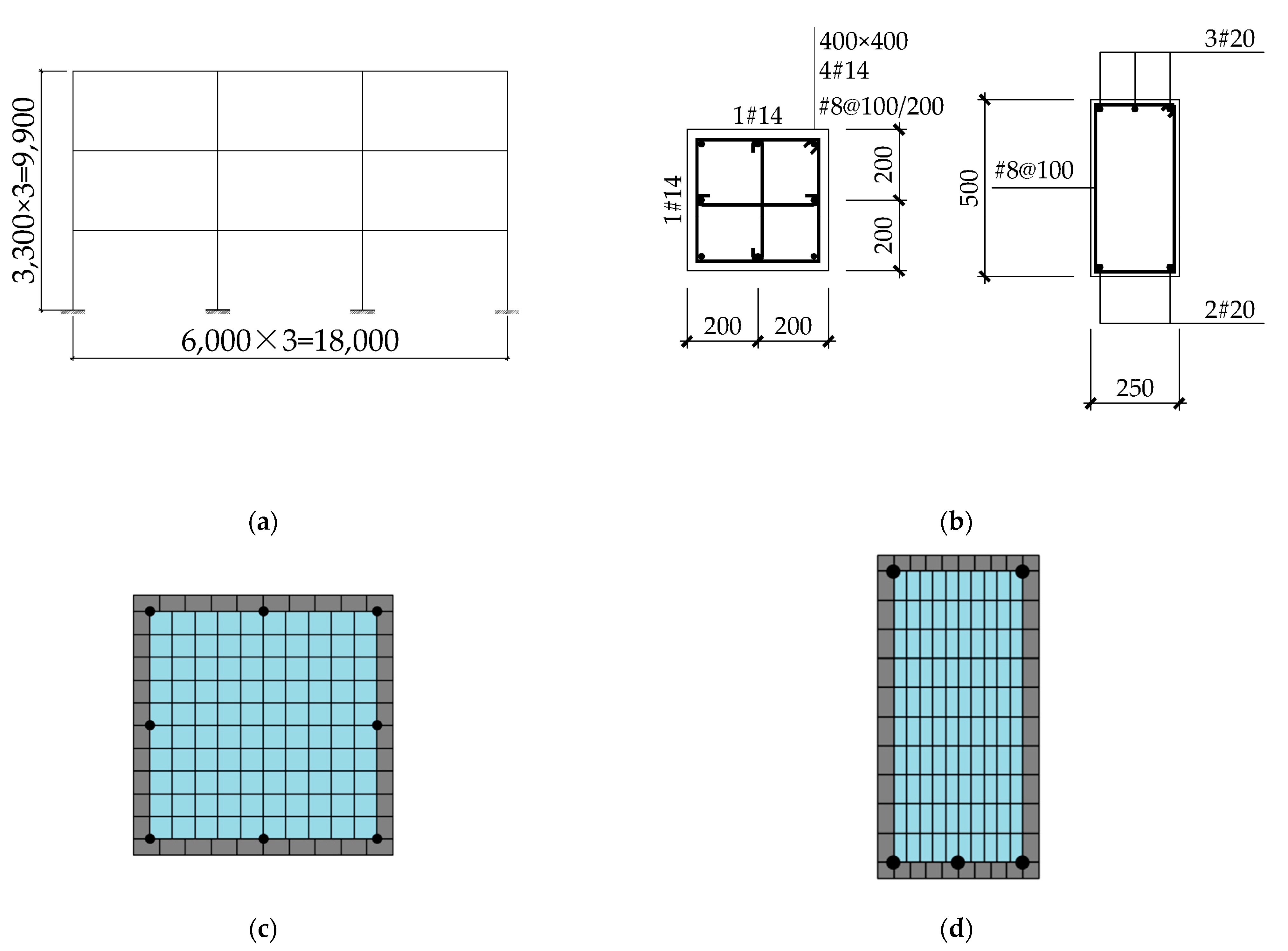
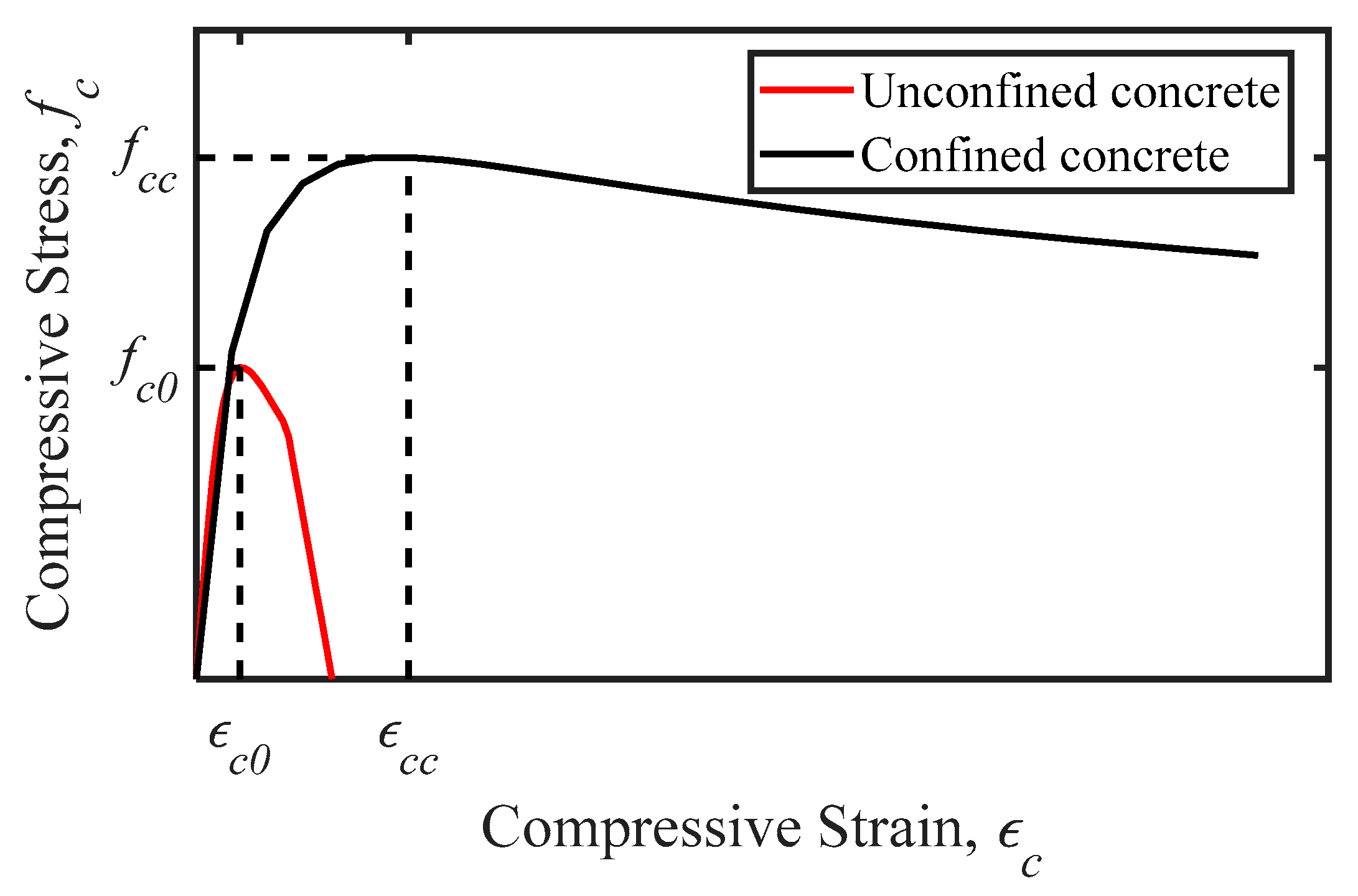
Figure 2a shows an example of the shape of a 2D RC frame. Figure 2b shows the column and beam sections that built this entire finite element model. Figure 2c,d show how the column and beam sections were meshed by the core and cover concrete in Opensees. The compressive strength of concrete is 30 MPa and the tension strength of steel is 400 MPa. In the column and beam sections, confined and unconfined concrete materials properties follow the Mander stress–strain model [40], as shown in Figure 3.
The relationship between the parameters in Figure 3 is:
f c = f c c x r r 1 + x r
In the Equation (18):
x = ε c ε c c
ε c c = ε c 0 1 + 5 f c c f c 0 1
f c c = f c 0 1.254 + 2.254 1 + 7.94 f 1 f c 0 2 f 1 f c 0
r = E c E c E s e c
E c = e c f c 0
E s e c = f c c ε c c
In the above equations, f c 0 is the unconfined concrete peak stress, ε c 0 is the unconfined concrete peak strain, f c c and ε c c are the confined concrete peak stress and strain, respectively; E c is the initial elastic modulus of concrete, E s e c is the secant modulus at the peak stress point; and f 1 is the effective restraint stress of the hoop reinforcement, which depends on the shape and strength of hoops:
f 1 = k e f 1
f 1 = 1 2 ρ s f y h
For rectangular hoops:
k e = 1 i = 1 n ω i 6 b c d c 1 s 2 b c 1 s 2 d c 1 ρ c c
In the above equations, ρ c c is the reinforcement rate of the longitudinal reinforcement in the core area of the hoop constraint; s is the net distance of the hoop; ω i is the net distance of the i-th longitudinal reinforcement; and b c and d c are the distances between the centerlines of the hoops along the two directions of the constraint concrete section.
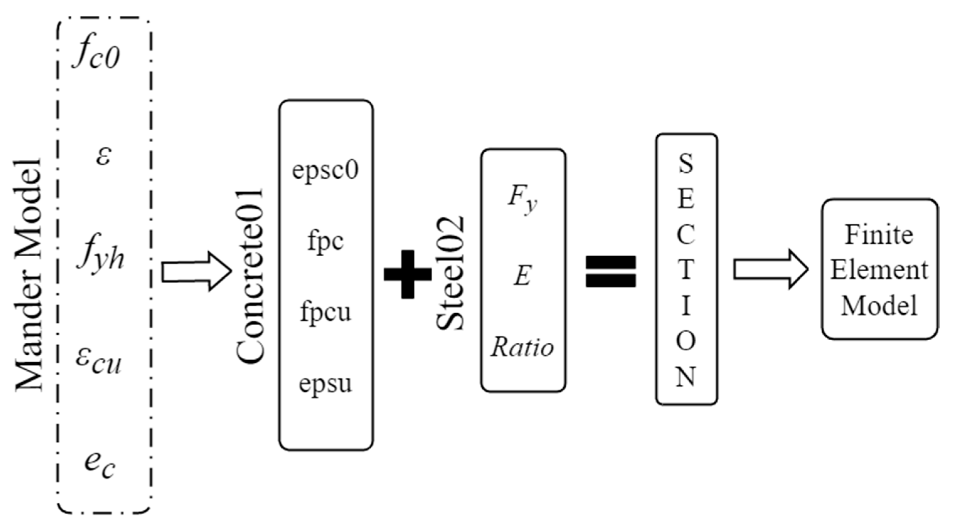
After performing the above calculations, these parameters are input to concrete 02 (a stress–strain rule in Opensees) to build the confined concrete materials.
For these reinforced concrete sections, steel materials properties follow the Giuffré-Menegotto-Pinto stress–strain model [40] (Steel 02 called in Opensees). Giuffré-nMenegotto-Pinto stress–strain model has four main parameters, f y , E , R, and Ratio, where f y and E are the yield strength stress and initial elastic modulus of steel. R is the parameter control for the transition from elastic to plastic branches, and Ratio is the value of plastic elastic modulus to the initial elastic modulus. Generally, they are set through a suggested value [41].
Derived from these previous Equations (18)–(27), to build a finite element model, the initial values of vector θ should be known.
The flowchart in Figure 4 shows how the FEM is built
θ = f c 0 , ε , f y h , ε c u , e c , F y , E , R a t i o

3.2. Structural Parameter Identification based on Nested Sampling

As shown in Figure 5, the input seismic recorder is I-ELC180 ground motion (obtained from the 1940 Imperial Valley earthquake at the Array #9 station). To prove the proposed method as much as possible, amplify the I-ELC180 ground motion PGA to 0.1 g, 0.3 g and input them into the FEM separately to create two different damage state cases (Case.1 PGA = 0.1 g, Case.2 PGA = 0.3 g). To simulate the acceleration collection in real engineering structures. The response acceleration data of the structural top story is recorded, and 20% root mean square (rms) [42] white noise is added to the acceleration to simulate collected responses in reality. It is easy to derive that, unlike the real structure, all the errors of FEMU in the numerical examples are oriented from the added white noise.

3.2.1. Initial Sampling and Structural Parameters Selection

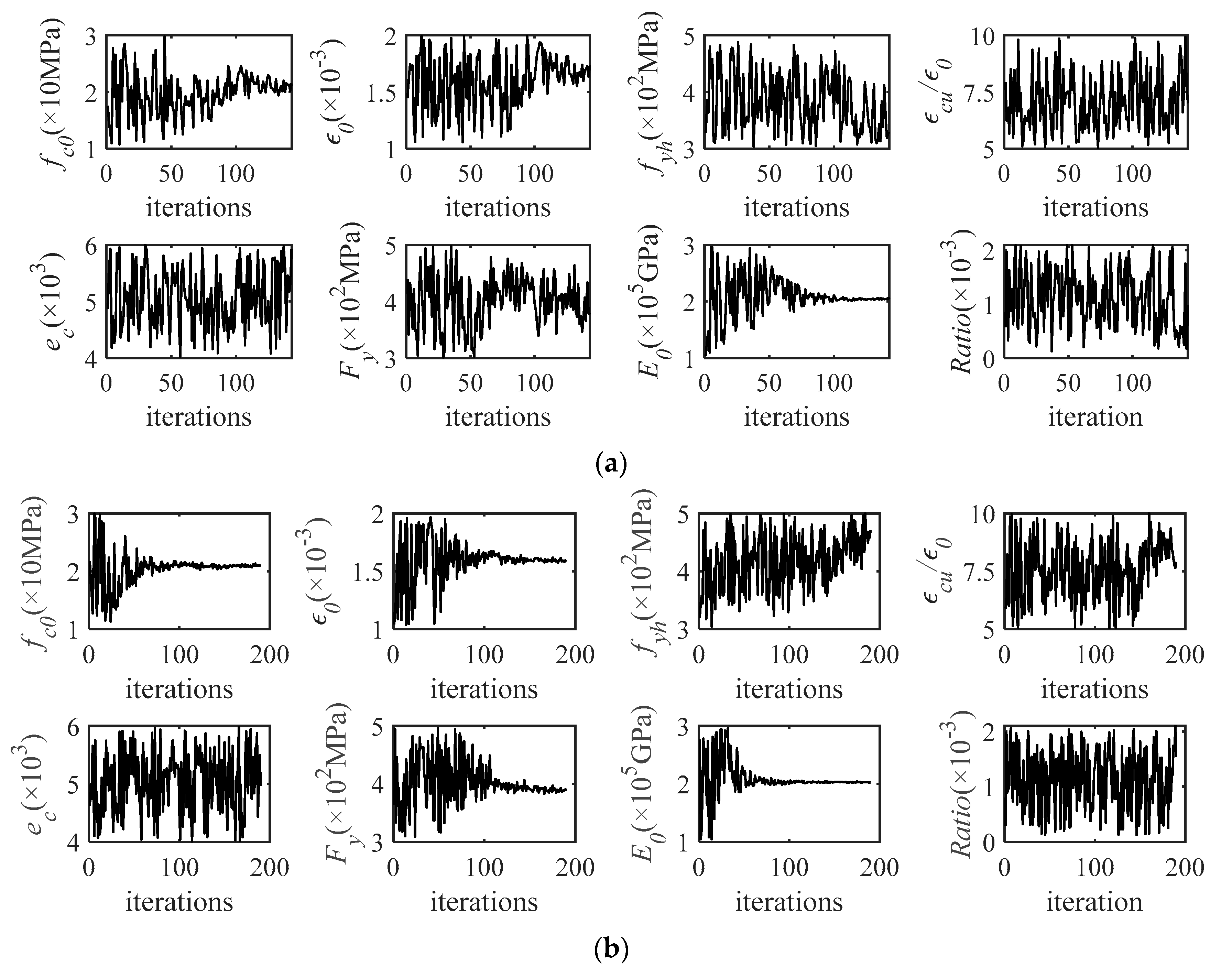
The simulated acceleration in Figure 5 is input to Equation (6), a large enough sample range, covering the parameter distributions range, is set to prior. The primary sampling is started using the method proposed in Section 2. The primary sampling process of different cases is shown in Figure 6.
In Figure 6a, it is evident that the parameters, such as ε 0 , f c 0 , and E 0 , have significant convergence in the iterative process, implying that the relationships between ε 0 , f c 0 and E 0 with the collected acceleration are strong. That is because, under the seismic force with PGA = 0.1 g, acceleration is barely collected with nonlinearity. In Figure 6b, it is evident that parameters, such as f c 0 , ε 0 , F y , and E 0 , are apparently gradually converging with the iteration; however, because the acceleration is nonlinear, the samples of f y h , ε c u / ε 0 , e c , and Ratio are different. Parameters such as F y affect the nonlinear time history. If we still insist on updating these parameters without a significant relationship, it will not only lead to inefficient sampling but may also produce incorrect results. Therefore, in FEMU, appropriate parameters should be selected for updating.
This paper recommends only sampling the parameters that are closely related to the collected information, such as ε 0 , f c 0 , and E 0 in Case 1. For the other parameters without close relationships, this paper recommends setting them as a suggested value.
The suggested value is defined using the historical data and engineering experience of the structure. For example, in this paper, the concrete which built the FEM was C30, and the Steel was HRB400. These suggested values in the FEM are shown in Table 1.
As described in Section 2, the primary sample process is similar to MLE. Therefore, we can record the last iteration’s acceleration response as y N , and substitute it into Equation (4) to calculate the standard deviation of error.
As mentioned in Section 2, considering the error as normal distribution and computing standard deviation, the standard deviation is estimated, which is shown below along with the true value.

3.2.2. Secondary Sampling

The selected parameters in the primary sampling are input into Equation (6). The stopping criterion is set as Equation (16). Then, sampling the modified equation as secondary sampling. The proposed approach is used to calculate the distribution of different parameters.
The results are as follows:
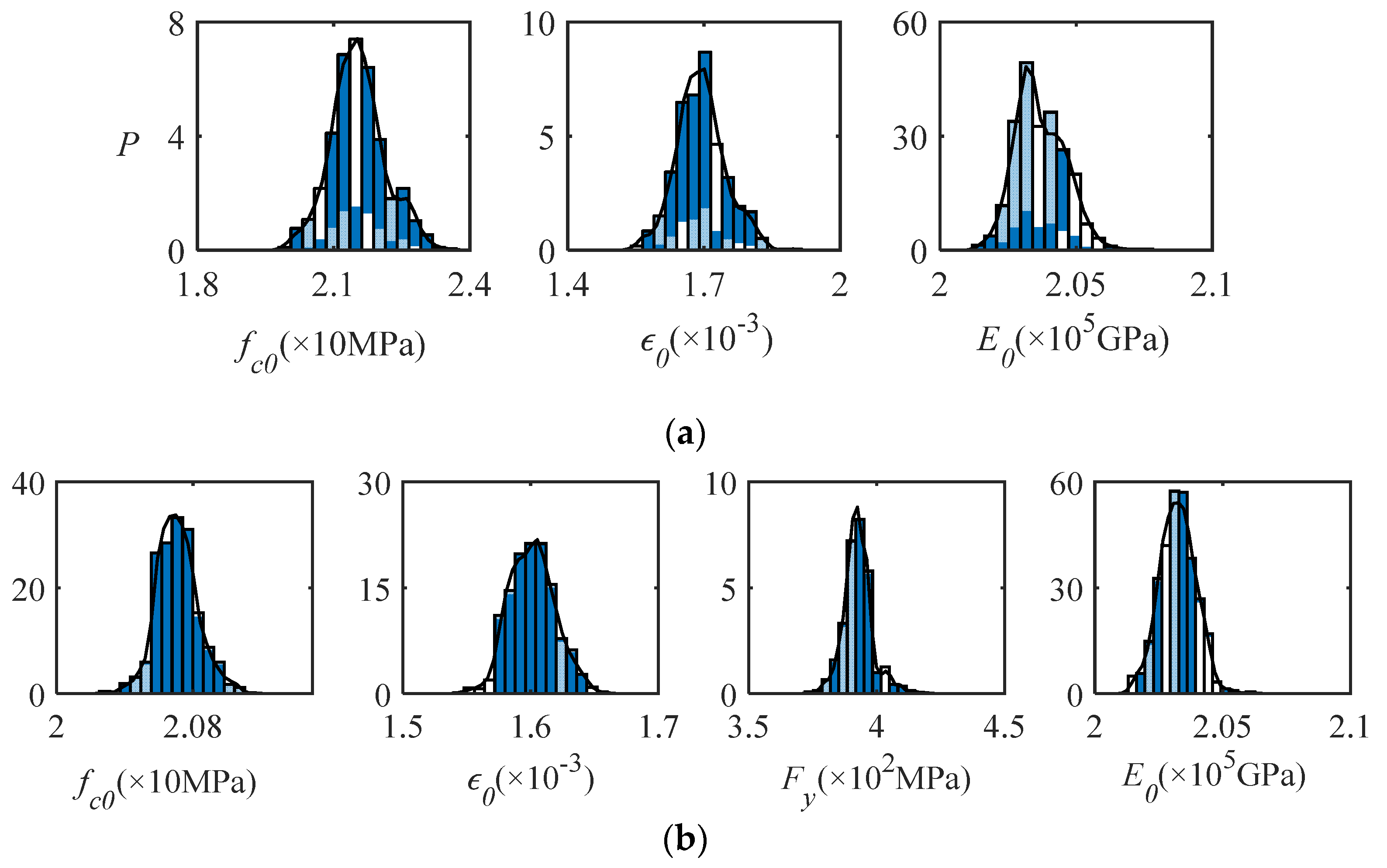
As shown in Figure 7, nested sampling successfully estimates the parameter probability density of the parameters and provides probabilistic FEM updating. To prove the reliability of the solution in different cases, this paper converted the error between the most likely estimated parameters in Figure 7 with true values.
As shown in Table 2 and Table 3, the sampling results have a small error of no more than 6% with these true values, implying that the results of the proposed method are reliable.

3.3. Damage State Estimation

The purpose of FEM updating is to accurately estimate the performances and damage state under an earthquake.
Mostly, the damage degree of the RC frame buildings is accomplished through the damage index as other structures. In general, the damage index can estimate the seismic damage degree of structural components and the whole body quantitatively. In recent years, a lot of calculated methods of damage index in long-term research have been proposed for different structures [43,44,45]. Actually, it is difficult to choose an adequate method to calculate the damage index, which can capture the damage level of structures using a single value. In this paper, because the model in the present research is simple, the seismic damage of the structure was expressed in the form of the Maximum Inter-Story Drift Ratio (MIDR), which is considered a useful damage index to estimate the RC Frame structural seismic damage [46].
In the case of RC frame building using MIDR to estimate the damage degree, Masi [47] proposed a relationship between MIDR and damage degree. As shown in Table 4 below, the damage state can be determined using the structural MIDR.
Similar to the parameters, the output responses of the FEM also have probability density. By inputting the ground motion to the FEM samples recorded in nested sampling and collecting the output MIDR of different models in samples, the distribution of the MIDR can be obtained. According to the probability density of the MIDR, the damage state of a structure’s underground motion can be obtained by integrating the probability density of the MIDR.
The MIDR probability densities of the 2D RC Frame Structure in different ground motion cases are shown below.
As shown in Figure 8, the MIDR estimated in Case 1 (PGA = 0.1 g) is in a null-damage-state MIDR range, and for Case 2 (PGA = 0.3 g), the estimated MIDR is in the Moderate-damage-state MIDR range; therefore, the estimated damage state probability is completely 100% Null and Moderate in different cases after the integral.
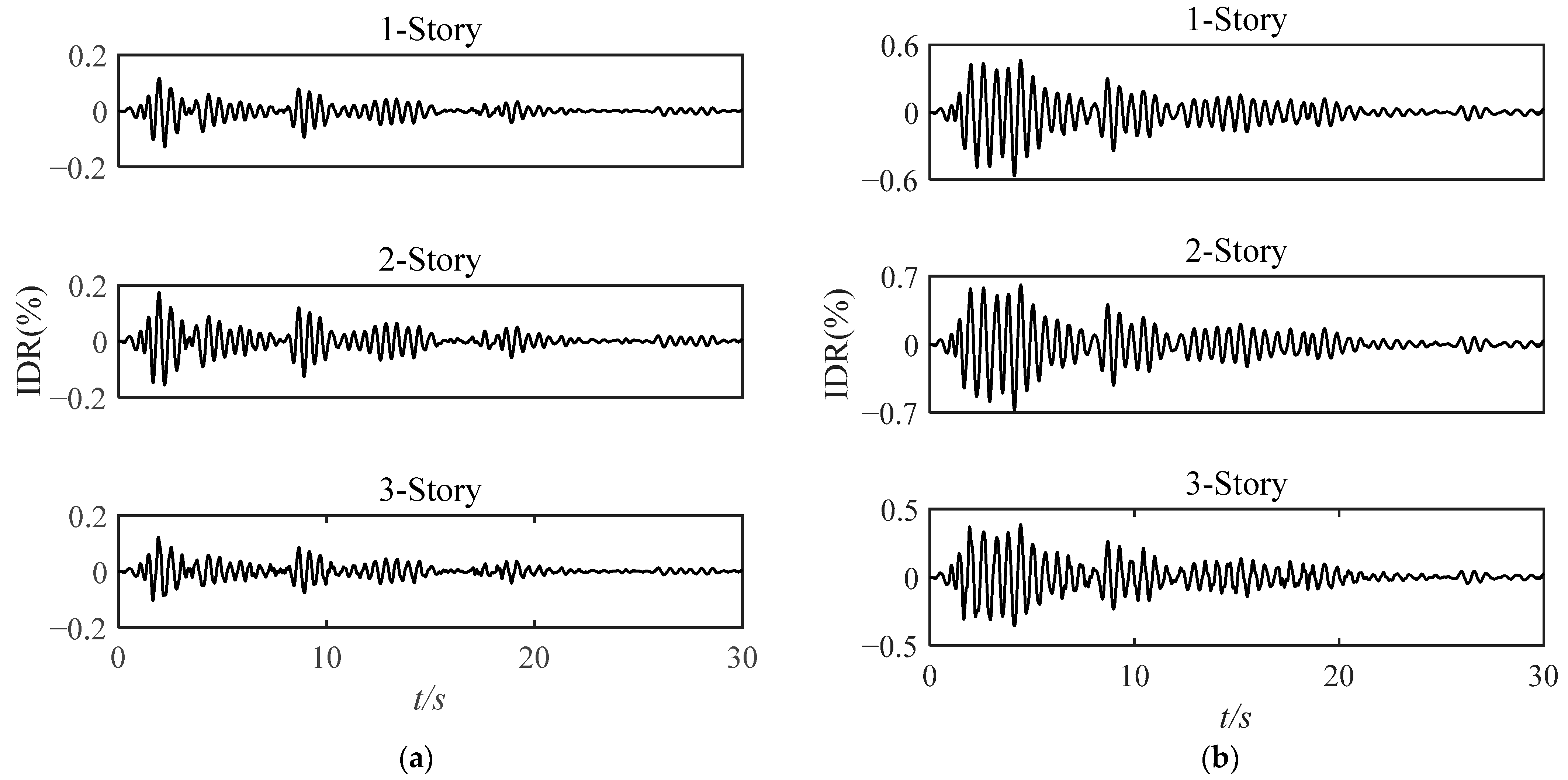
It’s easy for us to obtain the real Inter-Story Drift Ratio of the defined finite element model in different cases by Opensees. The output of the real IDR of the structure in different cases is shown in Figure 9 below.
As shown in Figure 9, the real max inner-story drift ratio and damage state in different cases are easily classified, and the results are shown in Table 5 below.
As we can see by comparing Figure 8 and Table 5, the real damage degree of the RC Frame FEM is null and moderate, which is as same as the estimated damage state. This implies that the proposed approach can successfully estimate the degree of structural global damage.
Furthermore, we can also calculate the MIDR probability distribution for each story using these output samples in nested sampling. Because the global damage degree of the structure, in the case of PGA = 0.1 g is null, there is no need to do further local damage degree analysis for the structure. Obviously, in the case of PGA = 0.1 g, the damage degree of each story in the structure is null. In the case of PGA = 0.3 g, the MIDR probability distribution of each story is calculated and shown below.
As shown in Figure 10, In the case of PGA = 0.3 g, we can deduce that the second story of the structure suffered the most serious damage compared with other stories. The estimated damage degree of the first story is the same as the second story, both are moderate damage. The third story of the structure estimate MIDR is in the range of 0.25–0.50, so the estimated damage degree of the third story is slight damage. This is the same as shown in Figure 9b.
Derived from the result, the proposed method can accurately locate the damage location and the damage state. In this result, it had not shown many probabilistic properties in estimating the structural damage state. This is because the error in the numerical example is too low to expand the range of sample distribution. This reason leads to an estimated results probability of 100%.

4. Conclusions

This paper proposed a FEMU approach by using nested sampling with nonlinear time history and its application in structural damage estimation. Different from other common sampling methods, the major advantage of the proposed method is that it can combine model selection with estimate probability distribution by changing the stop criterion.
The results from the example in different damage cases show that the nested sampling is reliable in the number of parameters’ reduction and selection without calculated evidence in different situations. This will help simplify high-dimensional space Bayesian problems in the future. Moreover, the results also show that the method could be used to estimate probability distributions by using the nonlinear time history and nonlinear models such as FEM, which is more advanced than other methods that are based on the Markov chain Monte Carlo approach.
We have also presented a method for damage probability estimation by using the samples created using nested sampling. It provided a new method to estimate damage state and location in probability.
The reliability of the proposed approach has been demonstrated by the numerical example in different cases. Because a large number of algorithms perform well in numerical examples but cannot be used in engineering, a real engineering structural example is still required to prove its application in the future. Future work will consider using the proposed method in the shaking table test and more complex structures, which have more parameters to estimate.

Author Contributions

Methodology, K.W.; Software, K.W. and Y.Y.; Investigation, K.W.; Writing—original draft, K.W.; Writing—review & editing, Y.K.; Funding acquisition, Y.K. All authors have read and agreed to the published version of the manuscript.

Funding

This research received no external funding.

Data Availability Statement

Conflicts of Interest

The authors declare no conflict of interest.

References

  1. Chopra, A.K.; Goel, R.K. A modal pushover analysis procedure for estimating seismic demands for buildings. Earthq. Eng. Struct. Dyn. 2002, 31, 561–582. [Google Scholar] [CrossRef]
  2. Vamvatsikos, D.; Cornell, C.A. Applied incremental dynamic analysis. Earthq. Spectra 2004, 20, 523–553. [Google Scholar] [CrossRef]
  3. Mander, J.B.; Dhakal, R.P.; Mashiko, N.; Solberg, K.M. Incremental dynamic analysis applied to seismic financial risk assessment of bridges. Eng. Struct. 2007, 29, 2662–2672. [Google Scholar] [CrossRef]
  4. Farrar, C.R.; Duffey, T.A. Bridge modal properties using simplified finite element analysis. J. Bridge Eng. 1998, 3, 38–46. [Google Scholar] [CrossRef]
  5. Friswell, M.; Mottershead, J.E. Finite Element Model Updating in Structural Dynamics; Springer Science & Business Media: BerlinHeidelberg, Germany, 1995; p. 5. [Google Scholar]
  6. Imregun, M.; Visser, W.J.; Ewins, D.J. Finite element model updating using frequency response function data: I. Theory and initial investigation. Mech. Syst. Signal Process. 1995, 9, 187–202. [Google Scholar] [CrossRef]
  7. Jaishi, B.; Ren, W.X. Structural finite element model updating using ambient vibration test results. J. Struct. Eng. 2005, 131, 617–628. [Google Scholar] [CrossRef]
  8. Marwala, T. Finite-Element-Model Updating Using Computational Intelligence Techniques: Applications to Structural Dynamics; Springer: London, UK, 2010; pp. 225–231. [Google Scholar]
  9. Ren, W.X.; Chen, H.B. Finite element model updating in structural dynamics by using the response surface method. Eng. Struct. 2010, 32, 2455–2465. [Google Scholar] [CrossRef]
  10. Abedin, M.; y Basalo, F.J.D.C.; Kiani, N.; Mehrabi, A.B.; Nanni, A. Bridge load testing and damage evaluation using model updating method. Eng. Struct. 2022, 252, 113648. [Google Scholar] [CrossRef]
  11. Li, W.; Yong, H.; Zikai, X. Machine Learning-Based Probabilistic Seismic Demand Model of Continuous Girder Bridges. Adv. Civ. Eng. 2022, 2022, 3867782. [Google Scholar] [CrossRef]
  12. Atalla, M.J.; Inman, D.J. On model updating using neural networks. Mech. Syst. Signal Process. 1998, 12, 135–161. [Google Scholar] [CrossRef]
  13. Levin, R.I.; Lieven, N.A.J. Dynamic finite element model updating using neural networks. J. Sound Vib. 1998, 210, 593–607. [Google Scholar] [CrossRef]
  14. Astroza, R.; Alessandri, A.; Conte, J.P. A dual adaptive filtering approach for nonlinear finite element model updating accounting for modeling uncertainty. Mech. Syst. Signal Process. 2019, 115, 782–800. [Google Scholar] [CrossRef]
  15. Behmanesh, I.; Moaveni, B.; Lombaert, G.; Papadimitriou, C. Hierarchical Bayesian model updating for structural identification. Mech. Syst. Signal Process. 2015, 64, 360–376. [Google Scholar] [CrossRef]
  16. Beck, J.L.; Katafygiotis, L.S. Updating models and their uncertainties. I: Bayesian statistical framework. J. Eng. Mech. 1998, 124, 455–461. [Google Scholar] [CrossRef]
  17. Li, X.; Kurata, M. Probabilistic updating of fishbone model for assessing seismic damage to beam–column connections in steel moment-resisting frames. Comput. Aided Civ. Infrastruct. Eng. 2019, 34, 790–805. [Google Scholar] [CrossRef]
  18. Lam, H.F.; Yang, J.H.; Beck, J.L. Bayesian operational modal analysis and assessment of a full-scale coupled structural system using the Bayes-Mode-ID method. Eng. Struct. 2019, 186, 183–202. [Google Scholar] [CrossRef]
  19. Jensen, H.A.; Millas, E.; Kusanovic, D.; Papadimitriou, C. Model-reduction techniques for Bayesian finite element model updating using dynamic response data. Comput. Methods Appl. Mech. Eng. 2014, 279, 301–324. [Google Scholar] [CrossRef]
  20. Beck, J.L.; Siu-Kui, A. Bayesian Updating of Structural Models and Reliability using Markov Chain Monte Carlo Simulation. J. Eng. Mech. 2002, 128, 380–391. [Google Scholar] [CrossRef]
  21. Ching, J.; Muto, M.; Beck, J.L. Bayesian Linear Structural Model Updating using Gibbs Sampler with Modal Data. In Proceedings of the 9th International Conference on Structural Safety and Reliability, Rome, Italy, 19–23 June 2005; Millpress: Rotterdam, The Netherlands, 2005; pp. 2609–2616. [Google Scholar]
  22. Cheung, S.H.; Beck, J.L. Bayesian Model Updating Using Hybrid Monte Carlo Simulation with Application to Structural Dynamic Models with Many Uncertain Parameters. J. Eng. Mech. 2009, 135, 243–255. [Google Scholar] [CrossRef]
  23. Boulkaibet, I.; Mthembu, L.; Marwala, T.; Friswell, M.I.; Adhikari, S. Finite element model updating using the separable shadow hybrid Monte Carlo technique. Top. Modal Anal. II 2014, 8, 267–275. [Google Scholar]
  24. Boulkaibet, I.; Mthembu, L.; Marwala, T.; Friswell, M.I.; Adhikari, S. Finite element model updating using the shadow hybrid Monte Carlo technique. Mech. Syst. Signal Process. 2015, 52–53, 115–132. [Google Scholar] [CrossRef]
  25. Lam, H.F.; Yang, J.H.; Au, S.K. Bayesian model updating of a coupled-slab system using field test data utilizing an enhanced Markov chain Monte Carlo simulation algorithm. Eng. Struct. 2015, 102, 144–155. [Google Scholar] [CrossRef]
  26. Zhao, Y.; Gong, M.; Zuo, Z.; Gao, Y. Bayesian estimation approach based on modified SCAM algorithm and its application in structural damage identification. Struct. Control Health Monit. 2021, 28, e2654. [Google Scholar] [CrossRef]
  27. Yuen, K.-V. Bayesian Methods for Structural Dynamics and Civil Engineering; John Wiley & Sons: New York, NY, USA, 2010. [Google Scholar]
  28. Skilling, J. Nested sampling. AIP Conference Proceedings. Am. Inst. Phys. 2004, 735, 395–405. [Google Scholar]
  29. Keeton, C.R. On statistical uncertainty in nested sampling. Mon. Not. R. Astron. Soc. 2011, 414, 1418–1426. [Google Scholar] [CrossRef]
  30. Speagle, J.S. Dynesty: A dynamic nested sampling package for estimating Bayesian posteriors and evidences. Mon. Not. R. Astron. Soc. 2020, 493, 3132–3158. [Google Scholar] [CrossRef]
  31. Jaynes, E.T. Prior probabilities. IEEE Trans. Syst. Sci. Cybern. 1968, 4, 227–241. [Google Scholar] [CrossRef]
  32. Xin, Y.; Hao, H.; Li, J.; Wang, Z.C.; Wan, H.P.; Ren, W.X. Bayesian based nonlinear model updating using instantaneous characteristics of structural dynamic responses. Eng. Struct. 2019, 183, 459–474. [Google Scholar] [CrossRef]
  33. Beck, J.L.; Yuen, K.V. Model selection using response measurements: Bayesian probabilistic approach. J. Eng. Mech. 2004, 130, 192–203. [Google Scholar] [CrossRef]
  34. Cao, T.; Zeng, X.; Wu, J. An arithmetic example study of nested sampling algorithm for groundwater model evaluation. Hydrogeol. Eng. Geol. 2017, 44, 69–76. (In Chinese) [Google Scholar]
  35. Myung, I.J. Tutorial on maximum likelihood estimation. J. Math. Psychol. 2003, 47, 90–100. [Google Scholar] [CrossRef]
  36. Terrell, G.R.; Scott, D.W. Variable kernel density estimation. Ann. Stat. 1992, 20, 1236–1265. [Google Scholar] [CrossRef]
  37. Douc, R.; Cappé, O. Comparison of resampling schemes for particle filtering Ispa 2005. In Proceedings of the 4th International Symposium on Image and Signal Processing and Analysis, Zagreb, Croatia, 15–17 September 2005; IEEE: Piscataway, NJ, USA, 2005; pp. 64–69. [Google Scholar]
  38. McKenna, F. OpenSees: A framework for earthquake engineering simulation. Comput. Sci. Eng. 2011, 13, 58–66. [Google Scholar] [CrossRef]
  39. Yang, Y.; Yang, Y.Q.; Zhao, Y.N. Comparative analysis of seismic capacity of RC frame structures based on different damage models. Earthq. Eng. Eng. Vib. 2020, 40, 118–126. (In Chinese) [Google Scholar]
  40. Mander, J.B.; Priestley, M.J.N.; Park, R. Theoretical stress-strain model for confined concrete. J. Struct. Eng. 1988, 114, 1804–1826. [Google Scholar] [CrossRef]
  41. Filippou, F.C.; Popov, E.P.; Bertero, V.V. Effects of Bond Deterioration on Hysteretic Behavior of Reinforced Concrete Joints; Report EERC 83–19; Earthquake Engineering Research Center, University of California: Berkeley, CA, USA, 1983. [Google Scholar]
  42. Gasparini, D.A.; DebChaudhury, A. Dynamic response to nonstationary nonwhite excitation. J. Eng. Mech. Div. 1980, 106, 1233–1248. [Google Scholar] [CrossRef]
  43. Chen, G.; Wang, Z.; Zuo, X.; Du, X.; Gao, H. Shaking table test on the seismic failure characteristics of a subway station structure on liquefiable ground. Earthq. Eng. Struct. Dyn. 2013, 42, 1489–1507. [Google Scholar] [CrossRef]
  44. Zhang, S.; Gaohui, W. Effects of near-fault and far-fault ground motions on nonlinear dynamic response and seismic damage of concrete gravity dams. Soil Dyn. Earthq. Eng. 2013, 53, 217–229. [Google Scholar] [CrossRef]
  45. Zhong, Z.; Wang, Z.; Zhao, M.; Du, X. Structural damage assessment of mountain tunnels in fault fracture zone subjected to multiple strike-slip fault movement. Tunn. Undergr. Space Technol. 2020, 104, 103527. [Google Scholar] [CrossRef]
  46. Naeim, F. The Seismic Design Handbook, 2nd ed.; Kluwer Academic: Boston, MA, USA, 2011. [Google Scholar]
  47. Masi, A.; Vona, M.; Mucciarelli, M. Selection of natural and synthetic accelero- grams for seismic vulnerability studies on reinforced concrete frames. J. Struct. Eng. 2011, 137, 367–378. [Google Scholar] [CrossRef]
  48. Morfidis, K.; Kostinakis, K. Seismic parameters’ combinations for the optimum prediction of the damage state of R/C buildings using neural networks. Adv. Eng. Softw. 2017, 106, 1–16. [Google Scholar] [CrossRef]
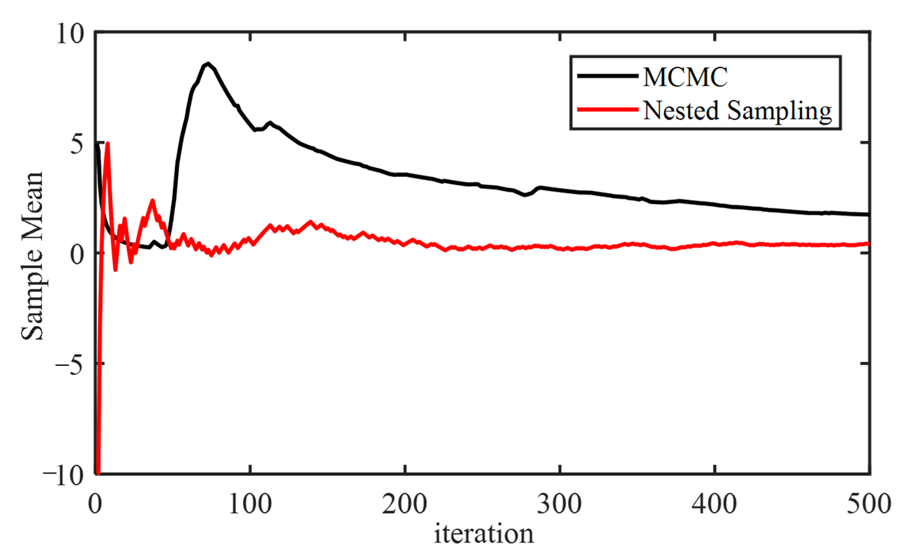
Figure 1. Sample Mean in Iteration Process.
Buildings 13 01281 g001
Figure 2. Two-Dimensional RC-Frame Finite Element Structure (unit: mm). (a) RC-Frame Structure; (b) Column and Beam sections; (c) Mesh of Column Section; (d) Mesh of Beam Section.
Buildings 13 01281 g002
Figure 3. Mander Stress–strain Model.
Buildings 13 01281 g003
Figure 4. FEM Build Flowchart.
Buildings 13 01281 g004
Figure 5. EL-Centro Ground Motion.
Buildings 13 01281 g005
Figure 6. Primary Sampling Process of Different Cases. (a) PGA = 0.1 g; (b) PGA = 0.3 g.
Buildings 13 01281 g006
Figure 7. Probability distribution of the parameters for different cases. (a) PGA = 0.1 g; (b) PGA = 0.3 g.
Buildings 13 01281 g007
Figure 8. Estimation of MIDR. (a) Probability Distribution of MIDR (PGA = 0.1 g); (b) Probability Distribution of MIDR (PGA = 0.3 g).
Buildings 13 01281 g008
Figure 9. Structural Real Performances in Different Cases. (a) IDR of Each Story (PGA = 0.1 g); (b) IDR of Each Story (PGA = 0.3 g).
Buildings 13 01281 g009
Figure 10. MIDR Probability of Each Story.
Buildings 13 01281 g010
Table 1. Suggested Value of Different Parameters.
ParametersSuggested Value
f c 0 (×10 MPa)2.01
ε 0 (×10−3)1.64
f y h (×102 MPa)4.00
ε c u / ε 0 7.00
e c (×103)5.00
F y (×102 MPa)4.00
E 0 (×105 GPa)2.06
Ratio (×103)1.00
Table 2. Comparison of the estimate and true value of the standard deviation.
STDEstimatedTrueError (%)
σ (PGA = 0.1 g)0.06950.06970.29
σ (PGA = 0.3 g)0.25370.25350.08
Table 3. Comparison of the estimate and true parameters.
CaseParametersEstimateTrueError (%)
PGA = 0.1 g f c 0 × 10   Mpa 2.012.135.97
ε 0 × 10 3 1.641.661.22
E 0 × 10 5   Gpa 2.062.031.46
PGA = 0.3 g f c 0 × 10   Mpa 2.012.072.99
ε 0 × 10 3 1.641.611.83
F y × 10 2   Mpa 4.003.951.25
E 0 × 10 5   Gpa 2.062.040.97
Table 4. Relation between the MIDR and damage state [48].
MIDR (%)<0.250.25–0.500.50–1.001.00–1.50>1.50
Degree of damageNullSlightModerateHeavyDestruction
Table 5. Structural Real MIDR and Damage State.
CaseMIDRDamage State
PGA = 0.1 g0.17Null
PGA = 0.3 g0.67Moderate
Disclaimer/Publisher’s Note: The statements, opinions and data contained in all publications are solely those of the individual author(s) and contributor(s) and not of MDPI and/or the editor(s). MDPI and/or the editor(s) disclaim responsibility for any injury to people or property resulting from any ideas, methods, instructions or products referred to in the content.