Performance Analysis of 3D Concrete Printing Processes through Discrete-Event Simulation

Abstract

Three-dimensional concrete printing is a technique that has been growing constantly, presenting advantages such as reduced completion times and a decreased environmental impact by eliminating the use of formworks. To carry out the process, the printing path of the extruded material and the movement of a robot must be programmed. Thus, the present research simulated these 3D concrete printing processes in a small 2-floor building of 309.06 m² and then in a 12-floor building of 10,920 m². To analyze the 3D printing process, discrete-event simulation was used while considering different variables such as extrusion speed and the locations of a robot mounted on tracks. The results show that when comparing the time taken for a conventional construction system to construct concrete walls and the maximum duration for 3D-printed walls, this method is 45% faster than traditional construction for a small building, but for a big building, there is a difference of 40% in favor of conventional construction; however, this was when using only 1 robot for the whole building. After running the same analyses but using 3 robots instead of 1, the total 3D concrete printing time for the big building was 80% faster in favor of the 3D concrete printing process.

1. Introduction

Three-dimensional printing is a technology that performs layered execution processes independent of the material used or a specific application. The American Society for Testing and Materials (ASTM) defines it as integrating materials to produce objects from a 3D data model, generally layer by layer, as opposed to traditional subtractive or assembly manufacturing methods [1,2]. This technology, which is applied to concrete printing using robots and integrative software, allows the creation of various geometric structures [3]. Hence, it is a technique that has revolutionized the creation of several products, processes, and services, showing its potential to be applied in a wide range of disciplines [4].

On the other hand, the construction industry presents certain deficiencies, such as poor energy efficiency in buildings, obstruction in work functions, and no digital management. As a result, diverse innovative practices have good prospects for enhancing the construction industry’s productivity and achieving a sustainable built environment [5]. Consequently, using new automated production technologies is necessary [6]. One of the initiatives to counteract these shortcomings is to promote the use of 3D-printed construction. This technology consists of an additive manufacturing (AM) process employing fluid–solid material deposition, which has recently become known thanks to the dissemination of experiments in different parts of the world [7]. In printed construction, robots are being utilized to print 3D concrete, helping to mitigate the sector’s shortcomings, and favoring the design of non-traditional architectural elements. In this way, it is essential to know where the robot can perform its work, evaluating configurations such as movement, speed, and trajectory to understand its scope and in which situations it can be used.

In the present investigation, an analysis was conducted based on the behavior of an ABB model IRB 6700-150/3.2 robot with 6 degrees of freedom, with a maximum reach radius of 3.2 m, mounted on a vehicle with a crawler undercarriage for its displacement [8]. It was assumed that the CYBE RC 3DP model of the company CyBe would be used [9].

It should be noted that this study considers that a mobile robot must settle in a stationary position to execute a continuous trajectory and then move to another location to print walls. Therefore, the robot’s position and sequence of locations are essential aspects to be considered when printing a building. The present study considered two residential buildings whose characteristics are shown in

Table 1. Characteristics of the residential buildings considered in this study.

	Small Building	Big Building
Number of floors	2	12
Area per floor	154.53 m2	910 m2
Total area	309.06 m2	10,920 m2
Height of the walls	2.75 m	2.75 m
Total height	5.5 m	33 m

.

It is worth mentioning that in the case of the big building, only one standard floor was analyzed, and its construction times and geometry were extrapolated to the other eleven floors. However, the small building was entirely analyzed on both floors. The choice of these two models to simulate (the small building and big building) was made based on the most common standard typologies in housing construction: residential houses and buildings. In terms of the dimensions used, the house (small building) was designed considering the maximum length of a long-range robotic arm (such as the one used in this study) and the least possible number of position changes. Then, the big building was an extrapolation of the small building, considering similar geometries that would make it possible to take full advantage of the versatility of the robotic arm under study (e.g., wide curves) and with the least number of position changes. The two simulated buildings are shown in Figure 1 and Figure 2.

In addition, in terms of the models considered as case studies, they were designed based on the great versatility and variety of shapes that 3D concrete printing (3DCP) processes provide [10], wherein the use of organic shapes and curves is an inherent biomimetic design concept [11]. In this sense, diverse researchers who work on 3DCP have been focused on creating innovative and challenging designs [12], including complex geometries such as domes with inclined layers, barrel vaults without external supports, or cantilevered structures with or without corbels [13]. However, in architectural and engineering design, there are still challenges related to building projects with curvilinear concrete shapes, wherein the use of 3DCP has become an interesting way to deal with these complex geometries [14].

Thus, the following research questions can be established: is it possible to evaluate the performance of 3DCP processes through the use of discrete-event simulation (DES)?; what are the main variables that should be considered when simulating 3DCP buildings?; and finally, through DES procedures, is it possible to estimate the total printing times of concrete houses and buildings, to compare them with conventional construction times? To help answer these questions, the main objective of this research was to analyze the performance of a mobile robot that prints 3D concrete walls under different configurations. The specific objectives were as follows: (a) to conduct a literature review to distinguish the state-of-the-art nature of 3DCP; (b) to define the most relevant variables involved in 3D printing times; (c) to design a model that simulates the behavior of a mobile robot printing 3D concrete walls; (d) to test different movement, speed, and trajectory settings in the simulation; and (e) to analyze and compare simulation times based on the different configurations.

2. Literature Review

2.1. Construction 4.0

Construction 4.0 has mainly focused on the digitalization and industrialization of the construction industry [15]. This concept provides a new technological approach that takes advantage of the automation of construction processes [16]. Therefore, to achieve a competitive advantage, many companies suggest the implementation of digital technological innovations, such as unmanned aerial systems, artificial intelligence, AM, and robotics, among others [17]. In this sense, some 3DCP applications combine AM and robotics, whereby their printing processes may be simulated.

2.2. Additive Manufacturing

AM is a technique whose term was formally adopted in 2009, encompassing all manufacturing techniques involving the addition of material using computational control until obtaining a durable product with a freedom of form that other methods do not allow [18]. This method may overcome traditional construction’s limitations, making it a new and advantageous technology [19]. In addition, it works without generating waste, resulting in a lower cost and a more sustainable production [20], along with improved energy efficiency and time savings [21]. Moreover, 3D printing is being integrated into various sectors of society (automotive and aerospace, medicine, food, construction, etc.) because of the customization and manufacturing of different products, allowing it to meet specific requirements.

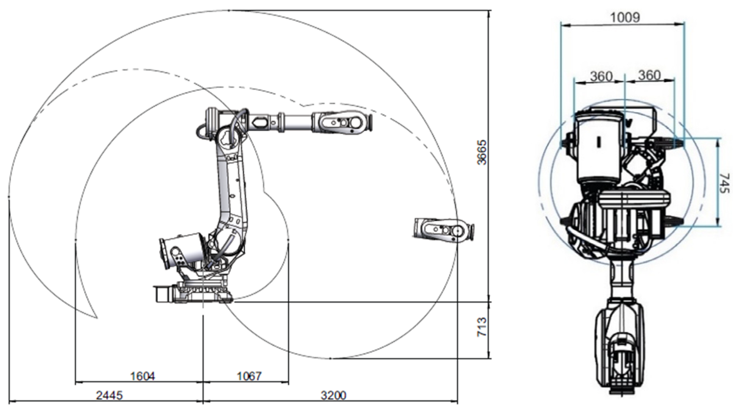
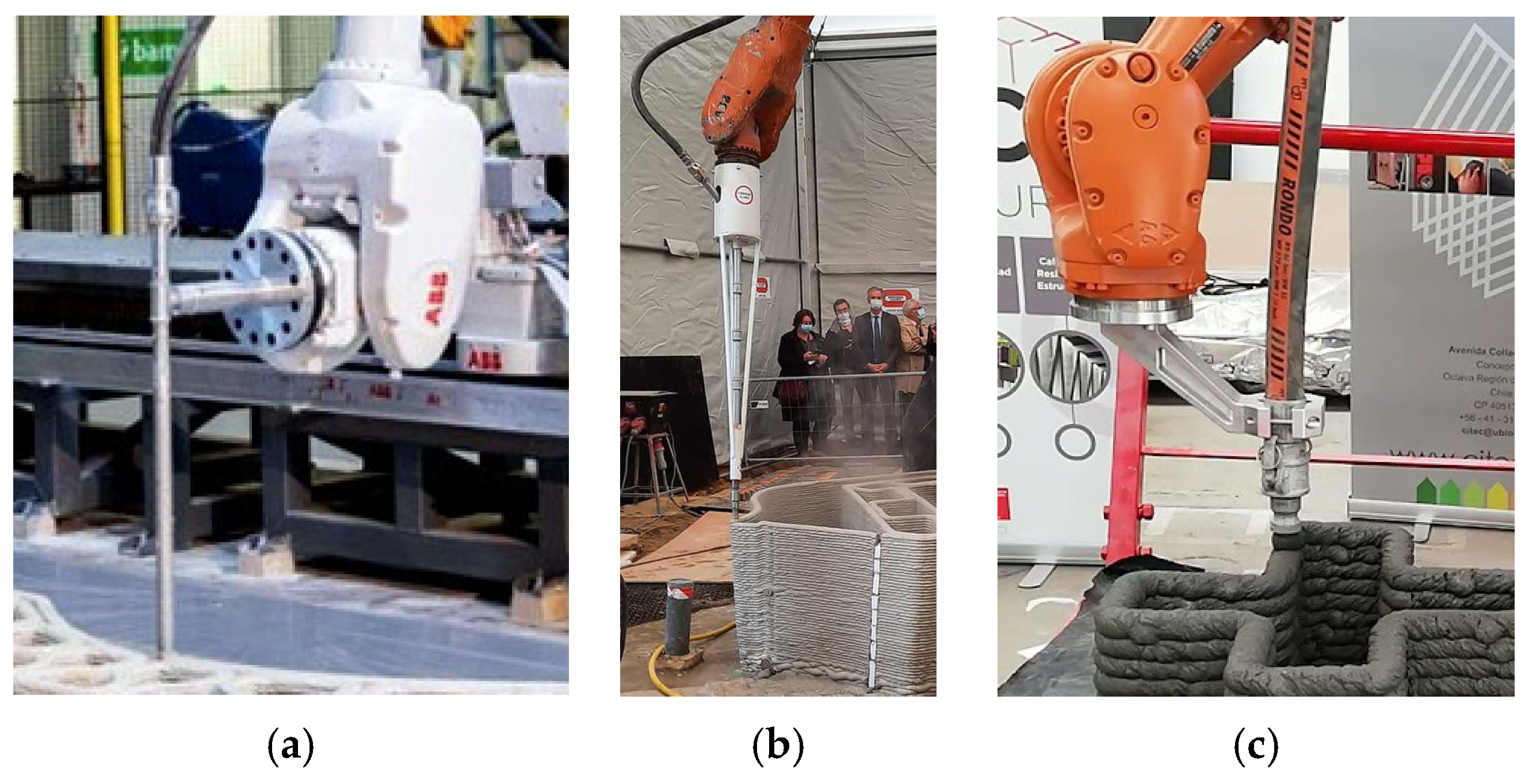
2.3. 3DCP and the Use of Robotic Arms

The term 3DCP has been used in the field of building and is called additive construction [22], and countries such as Japan and UK were the first to apply this technology in construction [23]. Today, there are three available manufacturing techniques for 3DCP: (1) D-Shape; (2) concrete printing, and (3) contour crafting [2]. In turn, different types of mechanisms are used to facilitate the deposition of 3D concrete, of which the following are the most relevant deposition technologies: (1) crane/gantry; (2) cable suspension; (3) mobile robots; and (4) robot arms [2]. There have been significant efforts to use robot arms in constructive processes, so the construction industry is implementing new technologies to modernize their traditional construction processes and thus facilitate the development of hazardous or tedious activities. The robotic construction of buildings, houses, or structures offers many advantages, such as a higher construction speed and a higher degree of customization [24].

2.4. Simulation of Processes

Process simulation attempts to mimic a given activity’s behavior through computing programs against different real situations. Due to the complexity of repeating the same conditions, attempts are made to approximate them so that the simulation is as close as possible to an existing event [25]. Currently, simulation software has the following characteristics: user interface, animation, and automatic results generating statistical analysis [26]. Thus, several simulations and process virtualization software can be found, such as (a) Arena; (b) Promodel; (c) Simul8; (d) KukaSim; (e) ExtendSim; (f) FlexSim, etc. On the other hand, several models are used as a foundation, wherein static and dynamic models stand out. It should be noted that dynamic models are divided into discrete, continuous, and discrete–continuous. Because of the nature of this study, based on the simulation of construction processes, we decided to use a discrete-event model to identify systems in which the variables change at specific instants of time [27]. This behavior determines that the simulation can be developed using a computer program pointing to events occurring in complex and stochastic systems [28].

In this sense, the activities that take place in construction can be discretized, for example, trucks entering or leaving the construction site, the concrete poured per hour, and the extrusion time [26]. Hence, since the aim was to analyze the performance of a mobile robot under different configurations when extruding, DES was used because of the following characteristics [29]: (a) discrete variables are used to simulate manufacturing processes; (b) in the simulation, graphical interfaces, animations, and automatic outputs are generated to measure the system’s behavior; (c) results can be analyzed as graphs or tables; and (d) in the statistical analysis, confidence intervals are included to study the behavior of the simulation results.

On the other hand, the construction industry constantly faces the challenge of increasing production to achieve stability over time and reduce costs [30], where simulation can contribute to dealing with these demands [28]. Thus, simulation applied to construction planning processes involves the creation of a model that represents how each of the activities developed in the execution of a project will be carried out. This tool has several applications that seek to improve the processes’ quality by studying each activity’s behavior [26]. The building process is performed through the development of numerous construction operations. In addition, this process is affected by the interactions between equipment, labor, and materials. Consequently, the project’s simulation and visualization arise, representing all the aspects that affect the construction process [31].

In summary, the advantage of developing a simulation is that it more appropriately represents the dynamics of construction processes since it considers randomness and variability in the results [32].

2.5. Simulation of AM Processes

The power of computers has increased significantly, and computer simulation has become a fundamental tool for researchers, whereby findings can be compared with experimental results after simulation to establish whether the models are accurate [33]. In other words, simulation has been a crucial tool in the evolution of 3D printing since it allows optimizing the design of parts, minimizing limitations in the fabrication method, and facilitating manufacture with the required quality and time [34]. In addition, it must be considered that such representation helps prevent errors and improves the quality of the processes. Hence, AM simulation for any material can be seen as a significant advantage in production because of its precision and quality in manufacturing parts. In short, 3D printing simulation and numerical modeling can decrease experiments through software, becoming as reliable as a physical test, in addition to offering lower costs and accurate information [35].

In terms of robotic AM process simulation, it provides the user with a visual tool before AM elements are made, helping with the design, characteristics analysis, and optimization of the AM process when the accuracy of the simulation is enhanced [36]. However, despite the importance of simulation in the construction engineering field, apart from the simulation of concrete structures, the majority of methods have not been intended for construction specifically [37]. Thus, there is limited evidence of a simulation methodology for AM processes for concrete, which would allow any professional in the construction sector to create their models simply and thus extend them to any construction project.

3. Methodology

The different stages that made it possible to carry out this research are presented below.

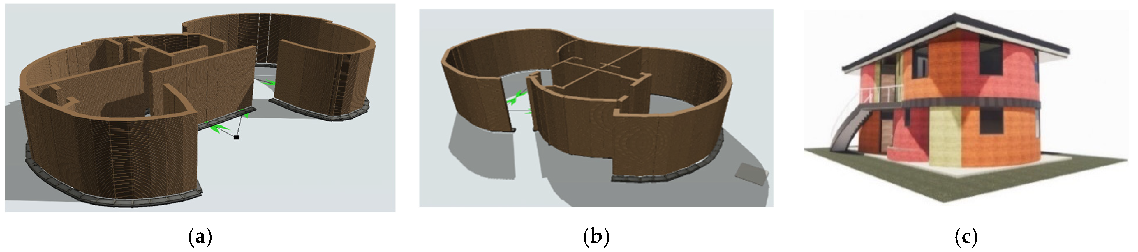
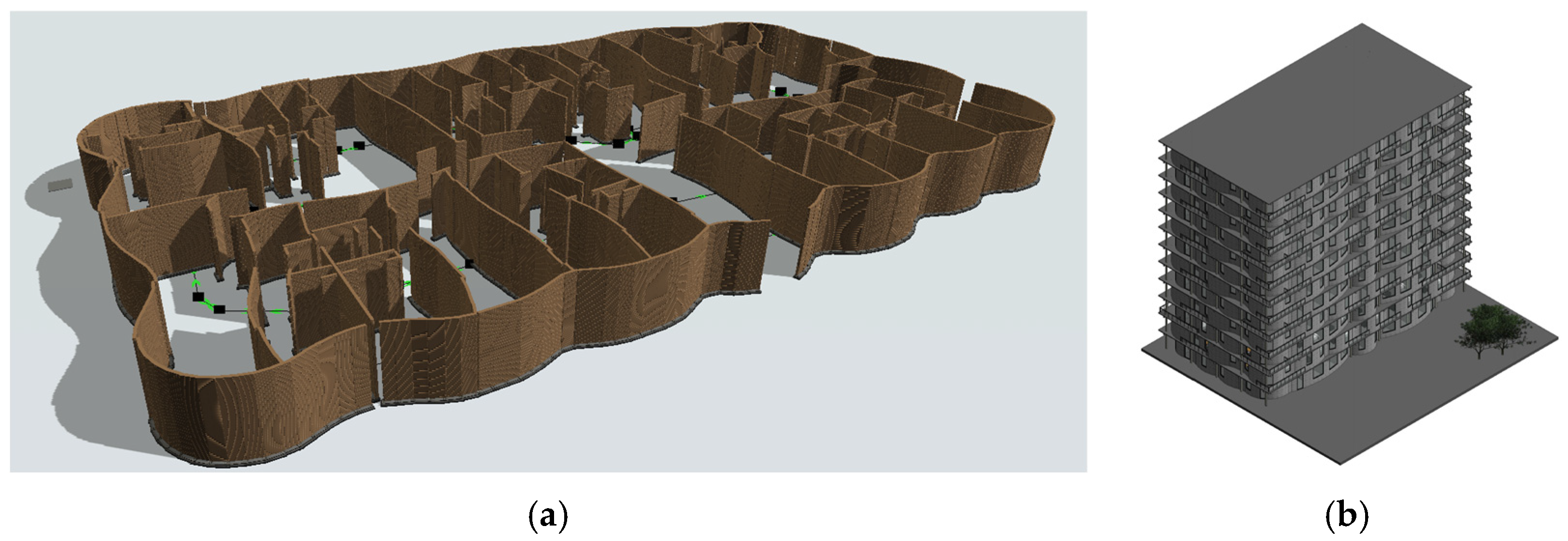
3.1. Modeling of Different Configurations for 3D Printing Concrete Walls

This section is subdivided into the following steps: export of the structural model from Revit to AutoCAD, analysis of the different possible locations for the mobile robot, and simulation of the different configurations and locations in the FlexSim^TM software (version 22.1, 2022, Orem, UT, USA).

3.1.1. Export of the Structural Model from Revit to AutoCAD

The robotic arm can work within a specific area, delimited by a maximum and minimum range radius. Therefore, it needs to be placed where it can cover as much area as possible from a single location.

The two models considered in this study were previously drawn in Revit. However, it was necessary to use AutoCAD software (version 24.1, 2022, San Francisco, CA, USA) to study the possible locations of the mobile robot because it facilitates the creation of designs using available drawing tools, such as lines and circles. At the same time, Revit focuses on creating construction models based on objects such as walls, slabs, and framing, among others. Additionally, FlexSim^TM reads .dwg files (created with AutoCAD) for use as a template, which is not present in Revit. Thus, the floor plans from Revit were obtained by exporting them to AutoCAD and then to FlexSim^TM.

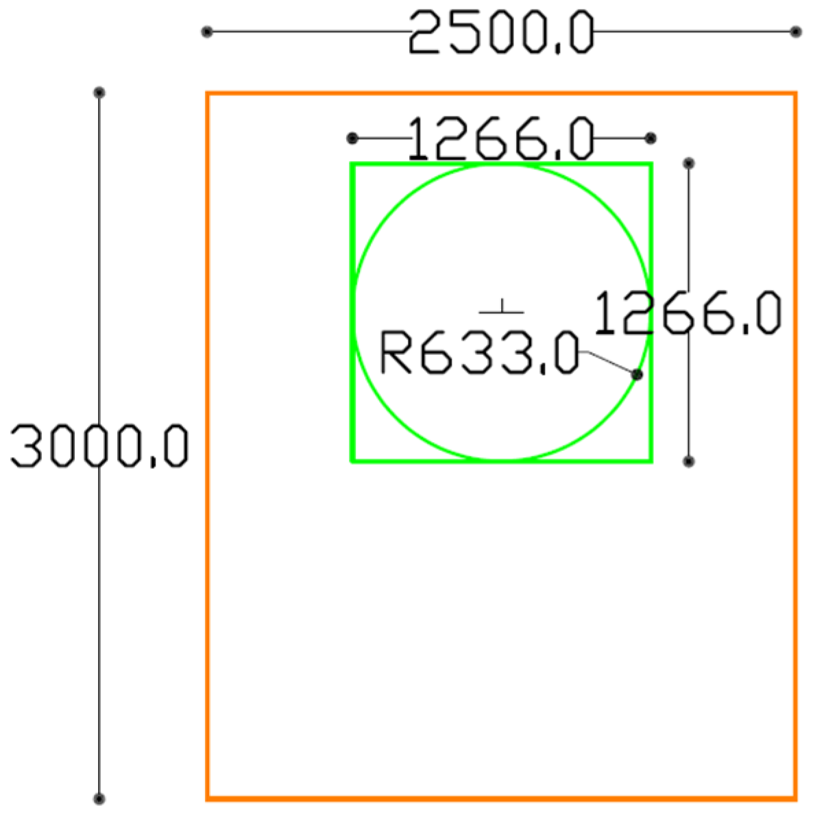
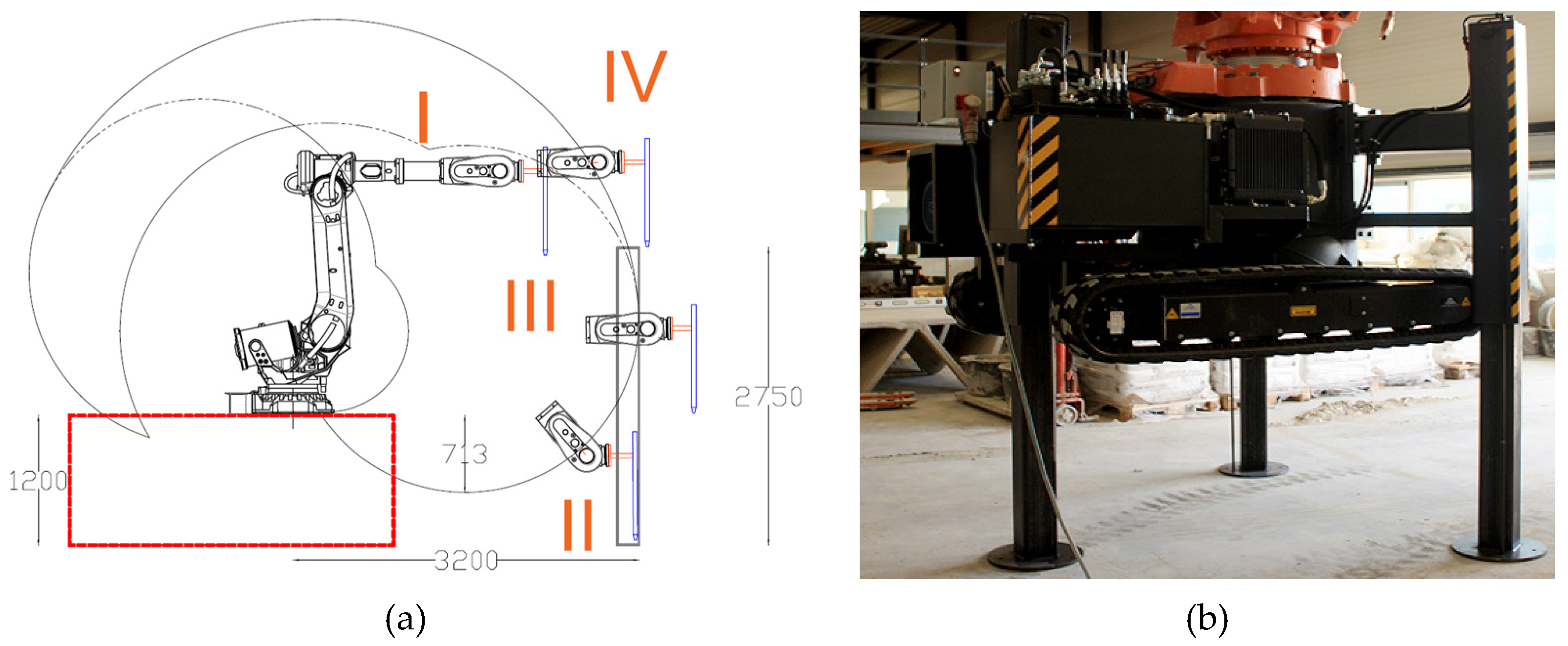
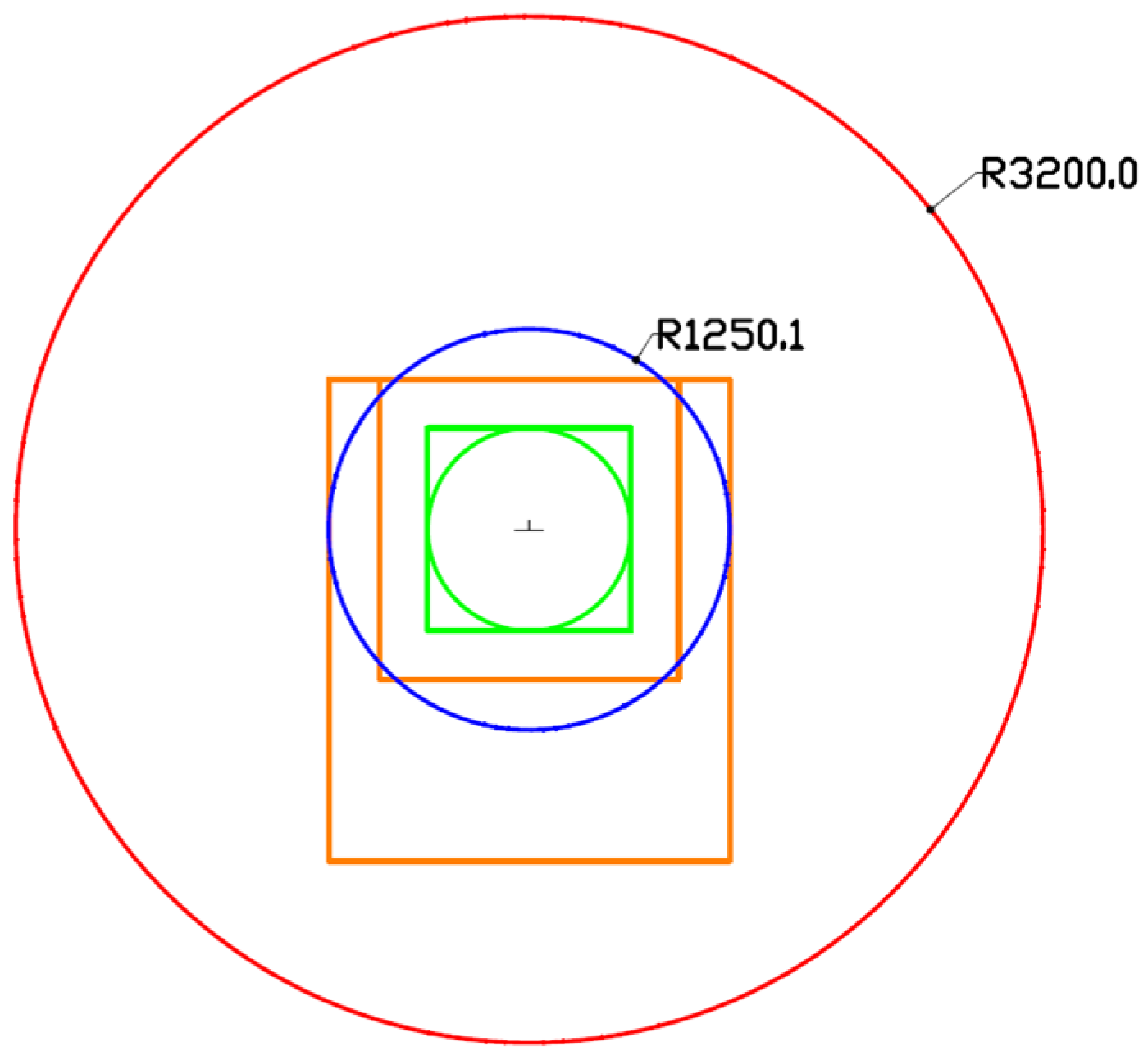
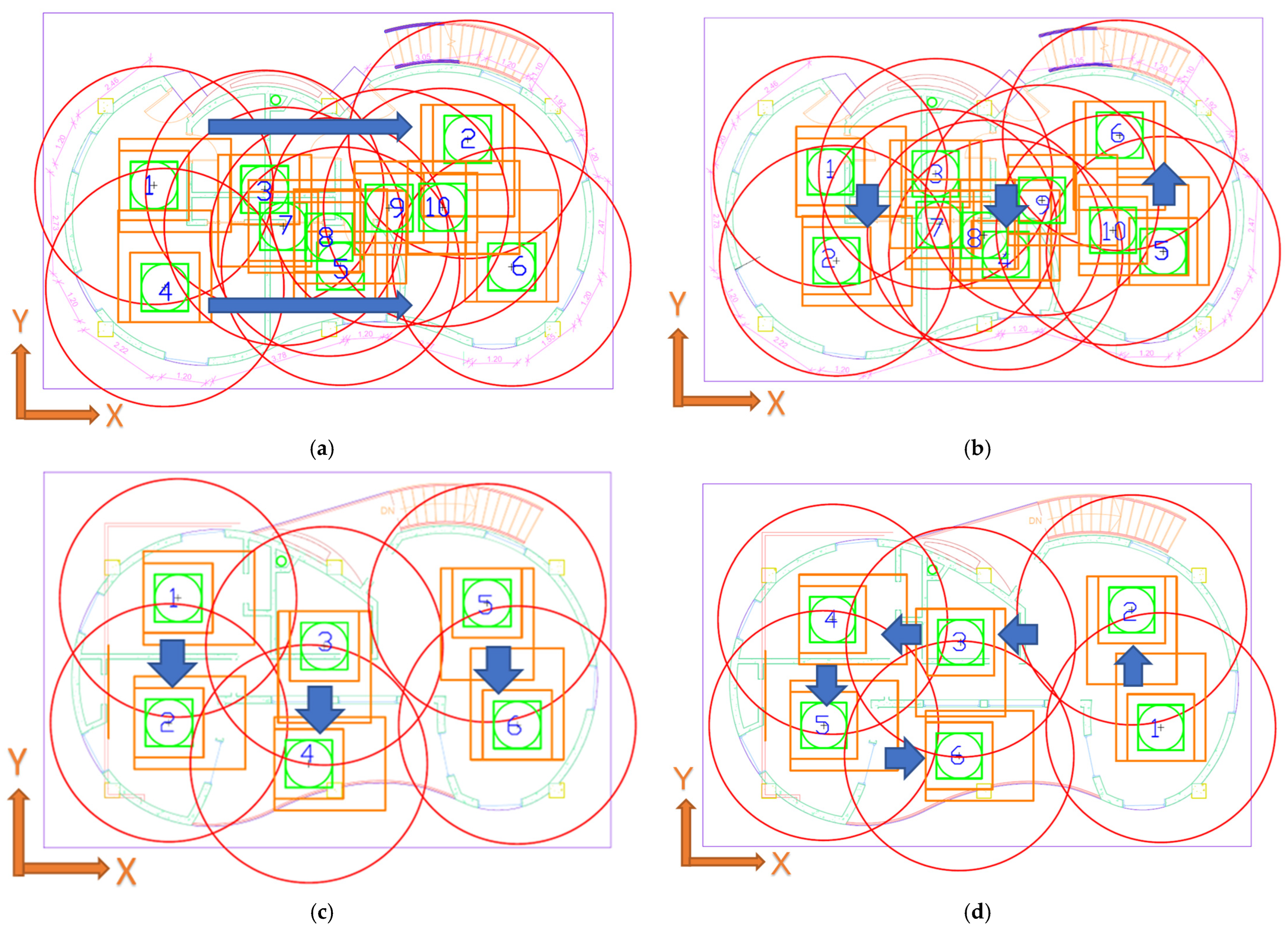
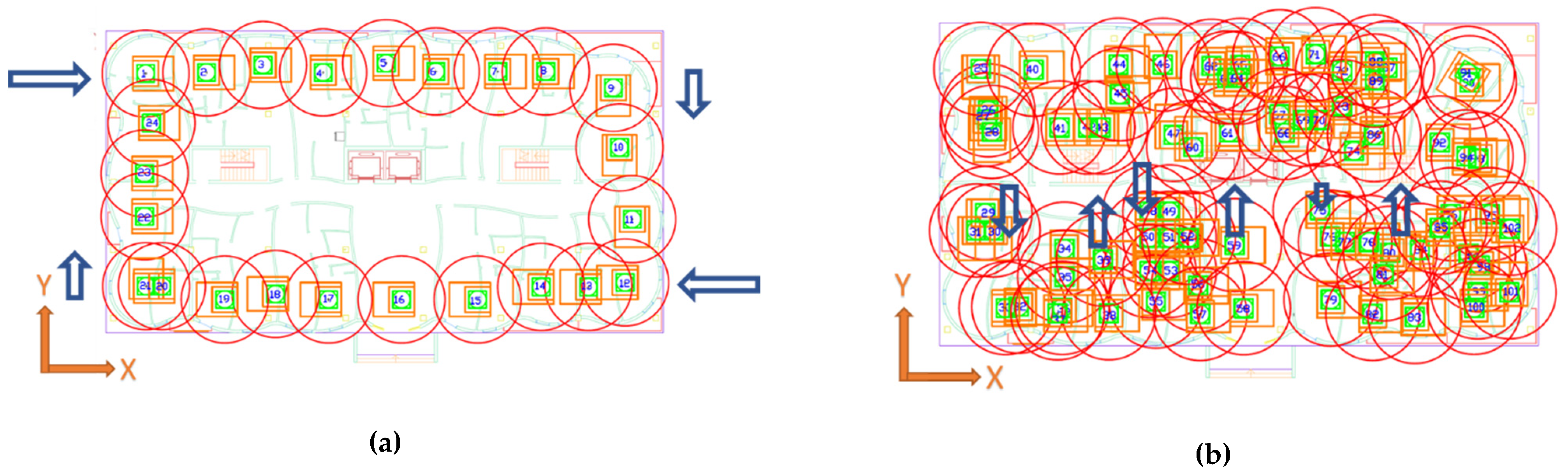
3.1.2. Analysis of the Different Possible Locations for the Mobile Robot

First, it should be mentioned that for this research, there were two ways to place the robot on the floor, such that a certain number of locations were obtained for each way. Thus, to better understand this study, the word “location” is understood as the number of locations the robot has on a floor plan to move from one location to another to complete the walls’ concrete extrusion.

Then, to know the area where the robot—and the tracked vehicle on which the robot is mounted—can operate, its dimensions were traced, and the best locations were established to allow covering most of the walls to be printed by emulating the behavior of a crane, as they work similarly. Next, the characteristics to be considered were proposed to know the crane’s strategic location point for use [38] (in this case, for the robotic arm).

(a)

Operational area for the robot

The operational area for a robot must not violate the inner limits or the outer limits of the floor, where the inner limits represent areas that are inaccessible for the device’s (crane or robot) positioning and operation due to existing structures. In contrast, the outer limit is defined as the area available for construction work and encompasses all structures on the site.

(b)

Device operation without collision

This area was required to ensure that the robot could rotate through 360°, including enough space for the device to lay down the concrete to be printed.

(c)

Starting points for motion trails

The following were the main characteristics of the device in charge of the printing process.

(1)

The mobile device must be located within the area of collision-free operation.

(2)

The maximum reach of the mobile device must overlap with the area on which to be worked.

(3)

When moving, the device must not collide with existing structures.

Accordingly, the possible mobile robot locations were analyzed, looking for the best positions that minimized the displacements and printed the entire structure. The robot’s range and dimensions were known [8] and are shown in Figure 3.

On the other hand, the CYBE RC 3DP CYBE tracked vehicle of the brand CyBe, which has a width of 3 m and a length of 2.5 m, was considered and is shown in Figure 4, where the green color represents the base of the robot, and the orange color represents the dimensions of the tracked vehicle.

It should be noted that the robot’s reach below the base was a maximum of 713 mm, which may have limited the extension of the arm; however, this was solved by adding a gripper to its tip, which is also called EOAT (end-of-arm tooling) and commonly used by companies such as ABB and CyBe. The function of the EOAT was to hold the extrusion hose and increase the reach for concrete deposition, some examples of which are shown in Figure 5.

In this way, and based on experimental tests carried out in situ, the robot reached the ground level beyond 713 mm due to the adjustments made in the field. On the other hand, considering that the EOATs were approximately 80 cm, it was possible to reach the floor level by contemplating the crawler’s height and the robotic arm’s characteristics.

To take advantage of the maximum performance of the robot’s reach, the tool shown in Figure 5a was considered. This configuration can be better appreciated in Figure 6a. In this figure, the movement that the robotic arm performs concerning the extrusion to build the concrete wall is shown graphically, wherein (I) is the initial position of the robotic arm before the extrusion; (II) is the robotic arm’s reach at the beginning of the extrusion; (III) is the robotic arm’s reach in the intermediate zone of the extrusion; and (IV) is the final robotic arm’s reach at the end of the extrusion. In addition, it should be noted that, if necessary, the chosen crawler vehicle could raise its height using hydraulic supports, as shown in Figure 6b.

Therefore, keeping in mind the robot’s reach, it was decided to operate outside the edges of the tracked vehicle, i.e., in a radius between 1250 mm and 3200 mm. The abovementioned range can be seen in Figure 7, where the blue circle represents the minimum range, and the red circle represents the maximum range in millimeters.

According to the above information, the walls must be printed entirely while avoiding collisions between the machine and the extrudate, thus obtaining different locations for the mobile robot.

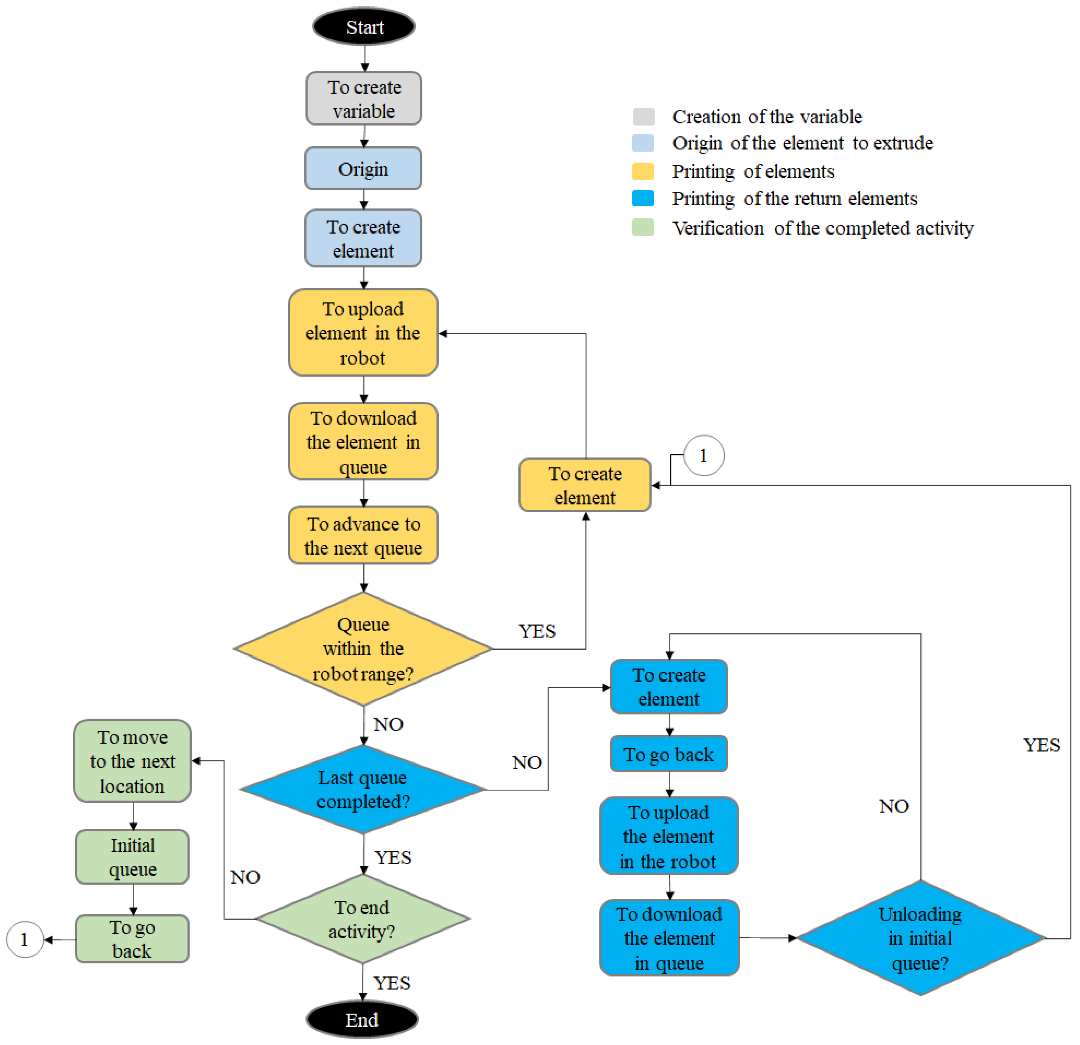
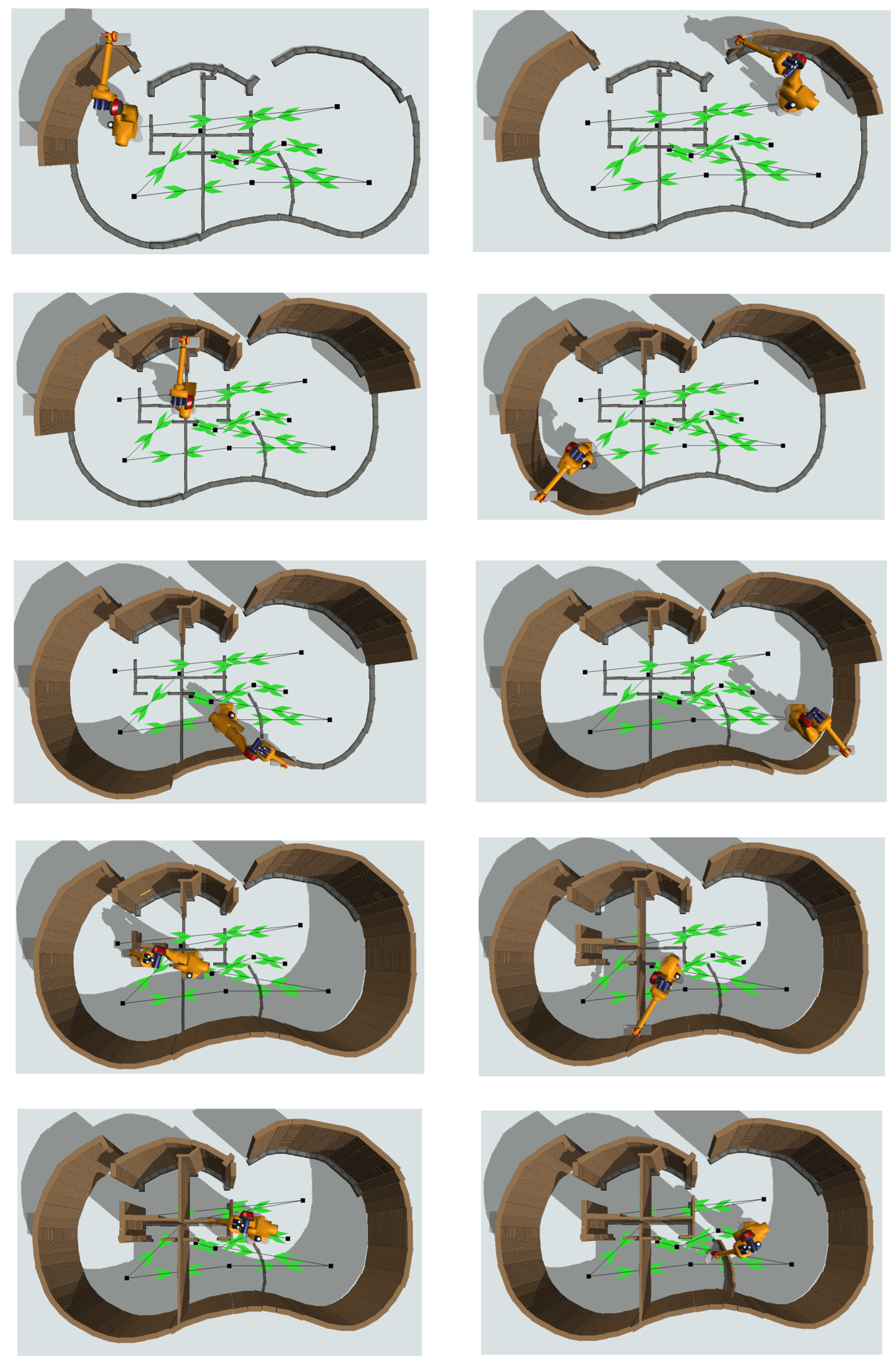
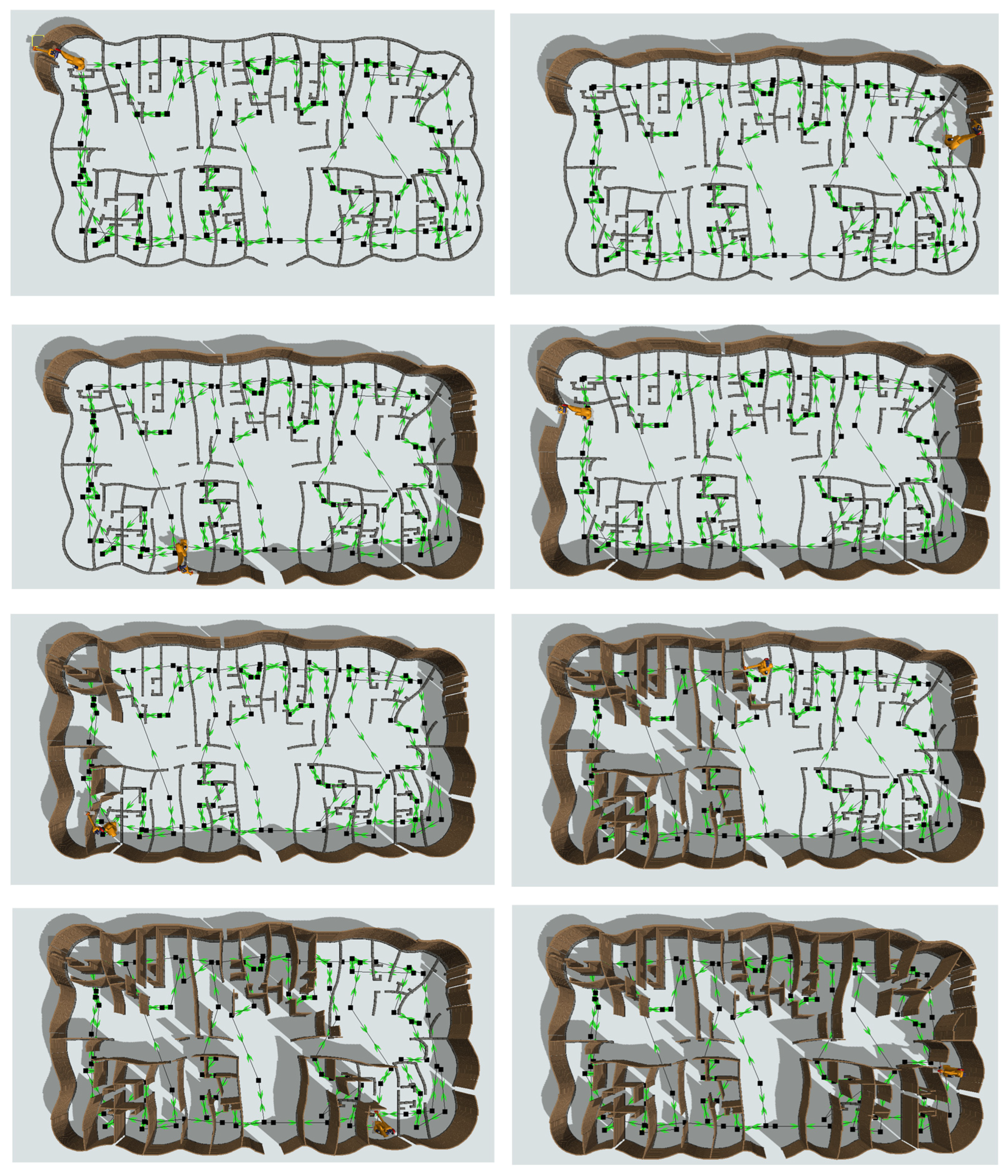
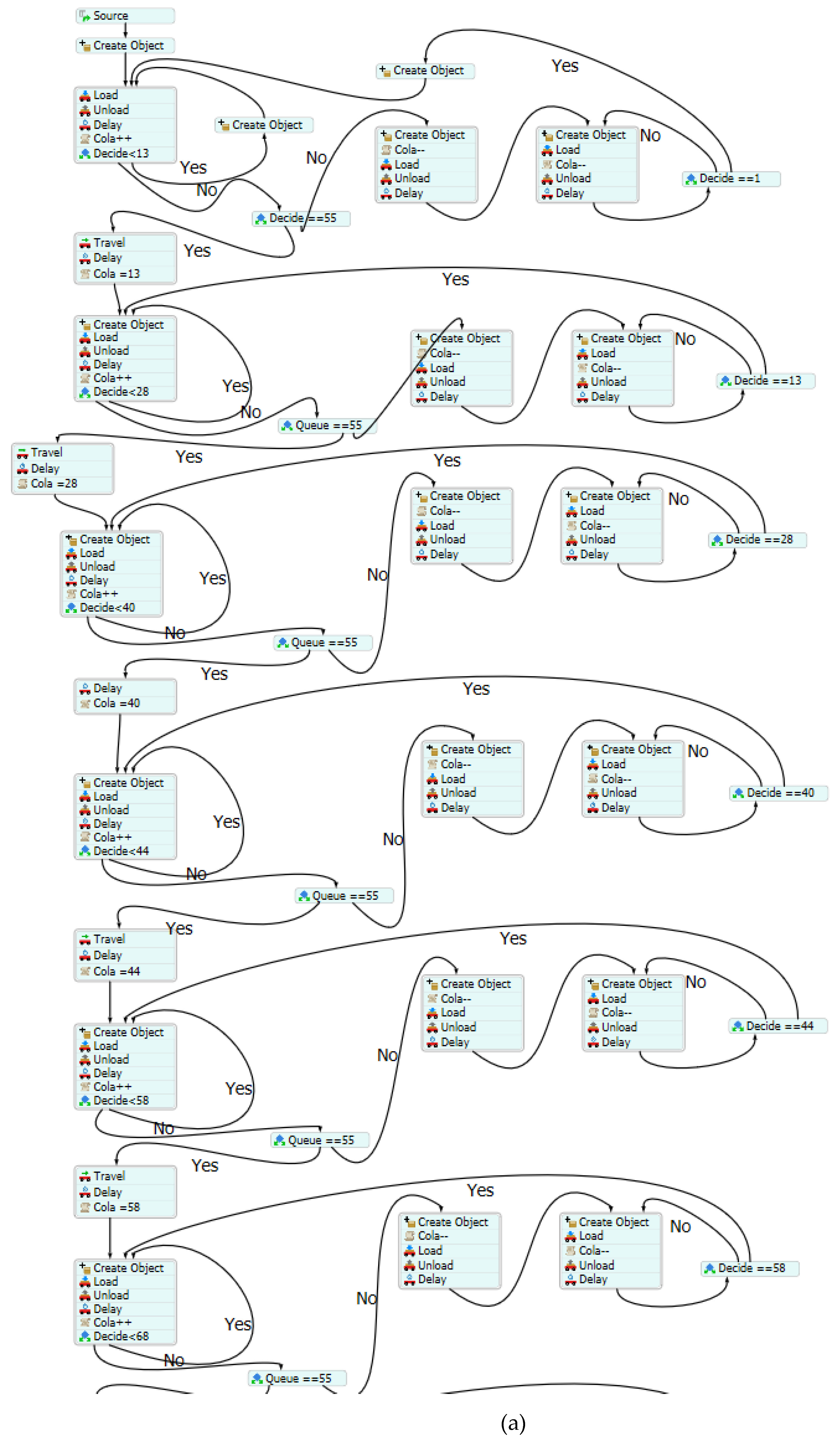
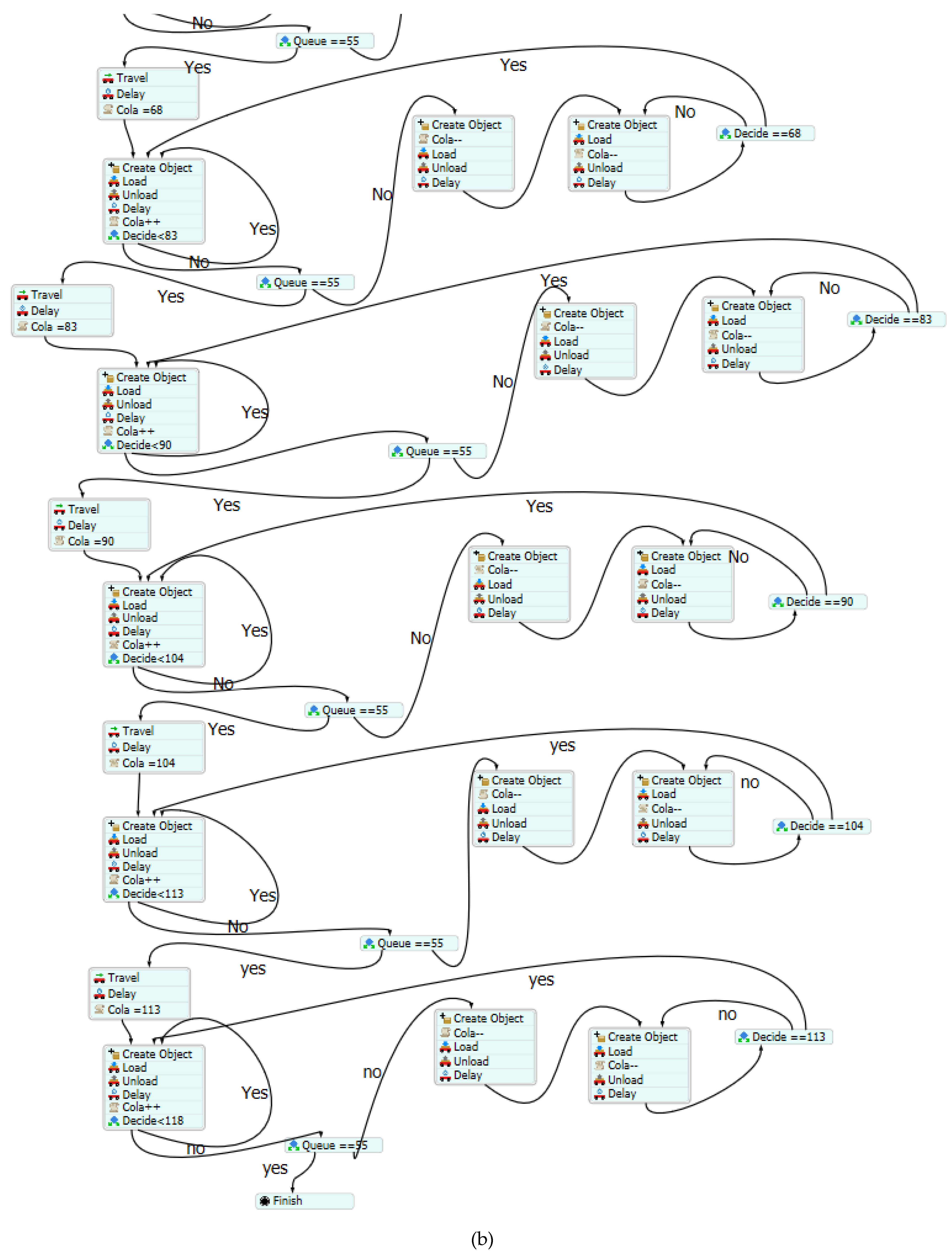
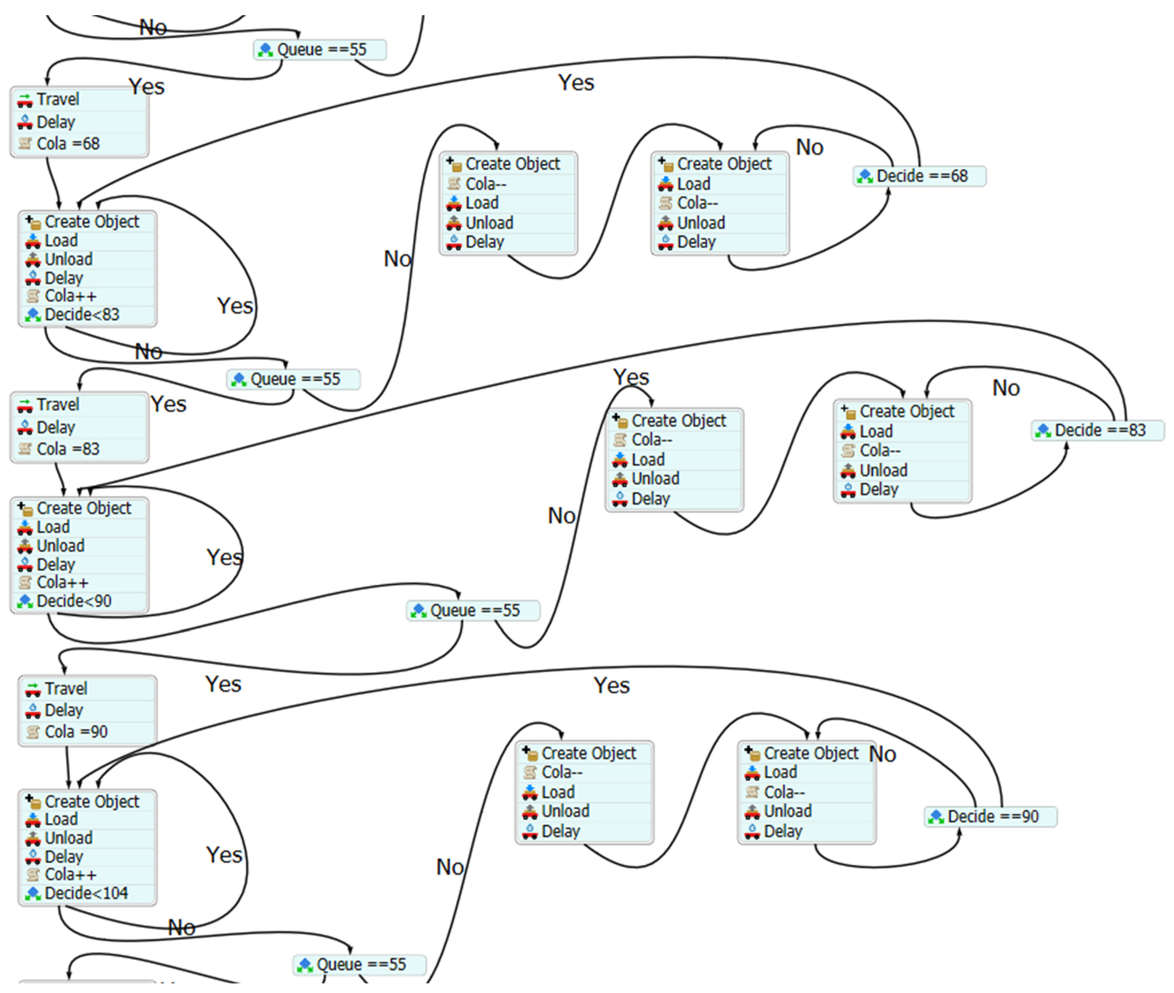
3.1.3. Simulation of Various Configurations and Locations in FlexSim^TM

FlexSim^TM is a DES program, while the robot extrudes continuously, so there may be a disjunction in their ways of working. However, the latter operates by placing the arm at specific points traced on the tracking path, as found in previous studies [10]. That is, the movement of the extrusion is continuous, but it is programmed to move with points of separation, that is, in a discrete way.

A simulation’s procedure must follow a flow that shows the path to carry out the simulation; therefore, a “Process Flow” must be created, which will be in charge of ordering the robot’s activities. Therefore, a flow chart was designed to encompass the methodology used, which was divided into groups characterized by colors (see Figure 8). These groups corresponded to the different operations that the robot must perform in the process flow.

Thus, an algorithm was implemented in FlexSim^TM according to what was defined in the flowchart. This code was explicitly run for the second floor of the small building; however, the process was the same for the rest of the floors, except for locations, trajectories, and movements, which do not need a different algorithm to be implemented. Furthermore, this procedure allows other work areas and scope for the robotic arm, which translates into different locations and queue nodes. The FlexSim^TM routines can be found in Appendix A. Therefore, the following provides an explanation of the groups shown in the flow diagram shown in Figure 8, and the code in FlexSim^TM can be found in Appendix A.

The floor plan of each building must be positioned as a template or “Background” as a reference to place the “Queue” in the area delimited by the walls, which will be responsible for containing the elements that simulate sections of the extrusion bead. Next, the robot that performs the task of depositing the material is inserted. Then the nodes are added, which mark the different locations and trajectories for the robot’s movement according to the different floor plans.

Later, the variable creation must be generated from the “Global Variable” option so that the robot knows in which “Queue” it must work. Then, at the origin of the material to be extruded, the element representing each point of the extrusion bead must be defined, where its dimensions and the resource from which it should originate are specified. For this purpose, the “Create Object” command is selected. Finally, the robot is programmed to move point by point, representing the concrete extrusion of the printed element. Herein, the specific parameters are also defined such as the robot’s printing speed, which depends on the wall geometry. Therefore, it was proposed that the wall width be divided by the bead width, depending on the nozzle size, to obtain the number of rounds of the printing bead, as shown in Equation (1).

$$n=\frac{B}{b}$$

(1)

where

• $n$ = the number of rounds of the printing bead;
• $b$ = Width of the printed bead (in meters);
• $B$ = Width of the wall (in meters).

Then, the length of the element to be deposited (l) is multiplied by n to determine the total length of the extruded bead (L), according to Equation (2):

$$L=n·l$$

(2)

where

• $n$ = the number of rounds of the printing bead;
• $L$ = Total length of the bead (in meters);
• $l$ = Length of the element (in meters).

Forcael et al. [10] experimentally analyzed the speeds at which a robot can print concrete, obtaining results of the speed versus spacing points. Thus, since the robot works according to the movement time, the period that the robot takes to print an element must be calculated according to Equation (3):

$$t=L·s$$

(3)

where

• $t$ = Time to extrude an element (in seconds);
• $L$ = Total length of the bead (in meters);
• $s$ = Printing speed of the robot (in meters per second).

Although robotic procedures are very accurate, a variation of ± 10% was considered to obtain maximum and minimum values using a triangular probability distribution —which is frequently chosen to represent at least uncertain activity durations and is widely used in project management to model events that take place within an interval defined with a minimum and maximum value [43,44]—, to obtain a potential variation in the total simulation time.

Another parameter to be configured corresponds to the travel speed of the tracked vehicle. For example, CyBe [9] and Giftthaler et al. [45] considered the maximum speeds at which a tracked vehicle operates when transporting an ABB robotic arm. In this way, different speeds were used to work with the minimum, average, and maximum values.

As a result, in FlexSim^TM, the “Load” command is adjusted to the mentioned speeds. In addition, a “Custom” code is added so that the robot advances the queue as it places the elements. Finally, to finish this stage, a “Decide” code is inserted to check if it reaches the last queue of the extrusion zone according to the position.

Then, in printing the next beads (one on another), the procedure of the previous stage is similar. The only difference is that, in this case, it is necessary to extrude in the opposite direction to the first bead because the robot is returning. This is performed once the last “Queue” of the printing sector is reached. Subsequently, a “Decide” code is inserted to check the number of elements in a specific queue that make up the height of the wall. If it reaches it, the robot must travel to the next position. Otherwise, if it does not reach it, the commands “Create Object”, “Load”, and “Custom” are entered. This last one is deployed so the robot decreases the correlative number of the “Queue”. Then, it reaches another “Decide” that checks if the first “Queue” of the extrusion site of such a location has been reached. If it has not, this last iteration is repeated; otherwise, it advances to the next position to continue with the next row. Later, the “Travel” and “Custom” commands are inserted in the completed activity verification. The abovementioned is carried out to travel to the next position, and the variable number is modified. In this way, the program can know in which “Queue” to start.

This process should be repeated as a pattern until the robot places the necessary elements in all the queues to simulate the extrusion of the whole floor plan. Finally, the FlexSim^TM “Experimenter” tool should be used to obtain different simulation times. In this case, 100 values were obtained and used in the statistical analyses.

3.2. Experimental Design

It was decided to consider 6 random values out of the 100 values obtained in FlexSim^TM. To introduce them as replicates in the factorial analysis, and to study the effects caused by the different configurations, a factorial-type experimental design with three factors was performed. In the factorial analysis, to analyze the performance of a mobile robot that prints 3D concrete walls, the three factors used were robot extrusion speed, crawler displacement speed, and type of location of the mobile robot, denoted by the letters A, B, and C, respectively.

The levels of each factor correspond to the minimum, average, and maximum robot extrusion speed and crawler displacement, A₁ being the minimum speed, A₂ the average speed, and A₃ the maximum speed at which the robot can work for the extrusion, whereas B₁, B₂, and B₃ are the travel speeds of the tracked vehicle, respectively. On the other hand, different ways in which the robot can be located were analyzed, where the locations were grouped into two types of locations: C₁ and C₂. In other words, each floor has two ways to place the mobile robot, C₁ and C₂, obtaining m and n numbers of locations, respectively. In summary,

Table 2. Test levels for each factor.

Factors	Coded Levels
A: Speed of the robot	A1	A2	A3
B: Speed of the crawler	B1	B2	B3
C: Location type	C1    C2

shows the factors and their respective levels in coded units.

According to the factors and levels each one takes, a 3 ∗ 3 ∗ 2 factorial design with 6 replications was applied, where 108 experimental points were obtained for each floor analyzed. Then, the analysis of variance and factorial graphs were derived from the statistical analysis of the results extracted from the simulation.

4. Analysis of Results

The previous chapter showed the strategy that was used through the analysis of the locations, the simulation in FlexSim^TM, and studying the most influential variables, resulting in simulation times. In this section, we will analyze those results.

4.1. Locations of the Robot

According to the methodology, two types of locations per floor were carried out. The results of the number of displacements concerning the locations and the robot movement direction are detailed below. It should be noted that for better identification of the analyses, they were designated according to the building, floor, and type of study, as shown in

Table 3. Nomenclature of the studies conducted.

Description	Type of Analysis
Small building, floor 1, analysis 1	S11
Small building, floor 1, analysis 2	S12
Small building, floor 2, analysis 1	S21
Small building, floor 2, analysis 2	S22
Big building, floor 1 (standard), analysis 1	B11
Big building, floor 1 (standard), analysis 2	B12

.

Thus, Figure 9 shows the configurations performed for S11, S12, S21, and S22 (small building).

As an example, Figure 10 graphically shows the printing sequence performed by the mobile robot for the extrusion of each of the walls in configuration S11 (the others are similar).

Then, the locations of the robot in the big building were analyzed. Figure 11 shows the configurations for the big building. In addition, as an example, Figure 12 graphically shows the printing sequence performed by the mobile robot for the extrusion of each of the walls in configuration B11 (the others are similar).

In this configuration (B12), 87 locations are determined for analysis type 1 and 102 for analysis type 2. Then, as shown in Figure 12, the robot prints the walls starting in the upper left corner, moving along the abscissa axis, and then returning for the next run.

4.2. Results of the Experimental Design

From the modeling in FlexSim^TM, for each configuration of robot extrusion speed and crawler travel speed, 100-time values were obtained that varied according to the triangular distribution considered for each test level, and in turn, for each location.

These results were used in two ways. First, the behavior of these figures was determined according to their variability. Then, the goodness-of-fit test was performed to determine which probability distribution fit each scenario. On the other hand, a factor analysis was performed to determine the most influential variables and their behaviors in different configurations.

4.2.1. Goodness-of-Fit

Related to the goodness-of-fit of the data, the following hypotheses were considered:

 Null Hypothesis a (H0a):

The time data fit a probability distribution.

 Alternative Hypothesis a (H1a):

The time data do not fit a probability distribution.

Based on these hypotheses, 100 data were taken from the simulation in FlexSim^TM, and a distribution fitting was performed using the Excel plug-in Crystal Ball^TM. Then, considering a confidence value of 95%, the null hypothesis would not be rejected when the p-values of the Anderson–Darling, Kolmogorov–Smirnov, and chi-square statistics were greater than a significance level α of 0.05. By comparing the p-value results with the given significance level, it was possible to accept the null hypothesis; therefore, the time data for each floor fit the probability distributions shown in

Table 4. Probabilistic distributions for each of the analyses studied.

Analysis	Robot Minimum Speed (0.1 m/s)			Robot Average Speed (0.225 m/s)			Robot Maximum Speed (0.35 m/s)
	Smin Crawler (0.3 m/s)	Savg Crawler (0.83 m/s)	Smax Crawler (1.4 m/s)	Smin Crawler (0.3 m/s)	Savg Crawler (0.83 m/s)	Smax Crawler (1.4 m/s)	Smin Crawler (0.3 m/s)	Savg Crawler (0.83 m/s)	Smax Crawler (1.4 m/s)
S11	Normal			Normal			Normal
S12
S21
S22
B11	Log-normal			Log-normal			Log-normal
B12

. Thus, the mean (µ) and standard deviation (σ) parameters per floor were obtained from the distributions fitted and shown in

Table 5. Average values and standard deviations of times in hours per floor according to the type of analysis.

Analysis	Robot Minimum Speed (0.1 m/s)						Robot Average Speed (0.225 m/s)						Robot Maximum Speed (0.35 m/s)
	Smin Crawler (0.3 m/s)		Savg Crawler (0.83 m/s)		Smax Crawler (1.4 m/s)		Smin Crawler (0.3 m/s)		Savg Crawler (0.83 m/s)		Smax Crawler (1.4 m/s)		Smin Crawler (0.3 m/s)		Savg Crawler (0.83 m/s)		Smax Crawler (1.4 m/s)
	µ	σ	µ	σ	µ	σ	µ	σ	µ	σ	µ	σ	µ	σ	µ	σ	µ	σ
S11	37.271	0.014	37.249	0.014	37.245	0.014	19.902	0.007	19.880	0.007	19.875	0.007	12.799	0.005	12.777	0.005	12.773	0.005
S12	37.260	0.014	37.245	0.014	37.244	0.014	19.891	0.007	19.876	0.007	19.875	0.007	12.788	0.005	12.773	0.005	12.772	0.005
S21	36.618	0.014	36.606	0.014	36.604	0.014	19.545	0.007	19.534	0.007	19.531	0.007	12.564	0.005	12.552	0.005	12.550	0.005
S22	36.617	0.014	36.606	0.014	36.603	0.014	19.544	0.007	19.533	0.007	19.531	0.007	12.563	0.005	12.552	0.005	12.550	0.005
B11	412.824	0.036	412.723	0.036	412.703	0.036	282.916	0.019	282.815	0.019	282.795	0.019	229.794	0.012	229.693	0.012	229.673	0.012
B12	409.996	0.036	409.807	0.036	409.769	0.036	280.995	0.019	280.806	0.019	280.768	0.019	228.244	0.012	228.055	0.012	228.017	0.012

.

According to Table 5, for S11, an average of 37,271 h was obtained when using the minimum speed. On the other hand, an average of 12,773 h was obtained for the maximum speed. For S12, these amounts corresponded to 37,260 and 12,772 h, respectively. In the case of S21, an average of 36,618 h and 12,550 h were obtained for the slowest and fastest configurations, respectively. Similarly, S22 had a minimum of 36,617 h and a maximum of 12,550 h. For the big building, in B11, the lowest average was 412,824 h, and the highest was 229,673 h. Thus, in B12, 409,996 h and 228,017 h were reached, respectively.

Now, the two floors of the small building behaved according to a normal distribution, with a low standard deviation, and the data values were close to the mean, so there was a slight variation. For the standard floor of the big building, a fit according to the log-normal distribution was found. Despite exhibiting a different fit, the standard deviation was also minimal, evidencing a low data variability. It should be noted that the big building consisted of 12 floors, where the standard floor (floor 1) was taken as a proxy for the rest.

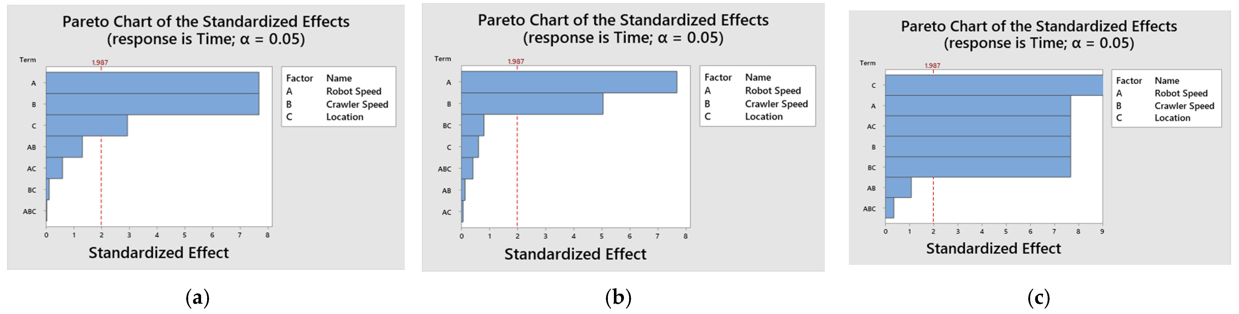
4.2.2. Factor Analysis and Variance

4.2.2.1. Factor Analysis of Three Factors

In the factorial analysis, six values were randomly taken to be used as replicates for each speed configuration and location. Thus, each floor time variation was obtained by combining these variables, at each test level, for each factor and considering the replicates. Appendix B (

Table A1. Simulation times in hours according to the combination of variables for floor 1 of the small building.

	A1									A2									A3
	B1			B2			B3			B1			B2			B3			B1			B2			B3
C1	37.28	37.27	37.25	37.26	37.25	37.27	37.25	37.23	37.25	19.89	19.89	19.90	19.88	19.88	19.88	19.87	19.88	19.88	12.80	12.79	12.79	12.77	12.78	12.78	12.78	12.77	12.78
	37.29	37.26	37.28	37.28	37.25	37.25	37.22	37.26	37.24	19.92	19.91	19.91	19.89	19.86	19.89	19.88	19.86	19.88	12.80	12.79	12.80	12.78	12.78	12.78	12.78	12.77	12.77
C2	37.26	37.27	37.25	37.23	37.26	37.24	37.25	37.20	37.22	19.90	19.90	19.90	19.86	19.86	19.89	19.89	19.87	19.88	12.79	12.78	12.79	12.78	12.78	12.77	12.77	12.77	12.77
	37.27	37.28	37.24	37.25	37.25	37.26	37.25	37.24	37.25	19.89	19.90	19.89	19.88	19.88	19.87	19.86	19.85	19.88	12.80	12.79	12.79	12.77	12.78	12.78	12.77	12.77	12.77

and

Table A2. Simulation times in hours according to the combination of variables for floor 2 of the small building.

	A1									A2									A3
	B1			B2			B3			B1			B2			B3			B1			B2			B3
C1	36.62	36.62	36.61	36.63	36.62	36.60	36.61	36.60	36.59	19.54	19.56	19.54	19.55	19.52	19.54	19.54	19.52	19.53	12.56	12.56	12.57	12.54	12.55	12.55	12.55	12.55	12.54
	36.61	36.61	36.62	36.58	36.61	36.59	36.60	36.62	36.62	19.54	19.53	19.55	19.53	19.54	19.55	19.53	19.54	19.53	12.57	12.57	12.56	12.55	12.56	12.55	12.55	12.56	12.55
C2	36.61	36.60	36.63	36.61	36.61	36.62	36.62	36.58	36.58	19.55	19.54	19.55	19.53	19.54	19.54	19.52	19.53	19.55	12.55	12.56	12.57	12.55	12.55	12.55	12.55	12.54	12.55
	36.65	36.60	36.60	36.61	36.62	36.59	36.60	36.60	36.61	19.54	19.54	19.54	19.53	19.52	19.54	19.53	19.52	19.53	12.57	12.57	12.56	12.56	12.56	12.55	12.54	12.55	12.54

) shows the variations for floors one and two in the small building. Similarly, for the big building,

Table A3. Simulation times in hours according to the combination of variables for the standard floor of the big building.

	A1									A2									A3
	B1			B2			B3			B1			B2			B3			B1			B2			B3
C1	412.8	412.8	412.8	412.7	412.7	412.7	412.7	412.7	412.7	282.9	282.9	282.9	282.8	282.8	282.8	282.8	282.8	282.8	229.8	229.8	229.8	229.7	229.7	229.7	229.7	229.7	229.7
	412.8	412.8	412.8	412.8	412.7	412.7	412.7	412.7	412.7	283.0	282.9	282.9	282.8	282.8	282.8	282.8	282.8	282.8	229.8	229.8	229.8	229.7	229.7	229.7	229.7	229.7	229.7
C2	410.0	410.1	410.0	409.8	409.9	409.9	409.8	409.8	409.8	281.0	281.0	281.0	280.8	280.8	280.8	280.8	280.8	280.8	228.3	228.2	228.3	228.1	228.1	228.1	228.0	228.0	228.0
	410.0	409.9	410.0	409.8	409.8	409.8	409.8	409.8	409.8	281.0	281.0	281.0	280.8	280.8	280.8	280.7	280.8	280.8	228.2	228.2	228.3	228.1	228.1	228.1	228.0	228.0	228.0

in the same Appendix B shows the simulation times according to the combination of variables for the standard floor (floor 1).

4.2.2.2. Factor Analysis of Three Factors

This analysis was carried out for each of the floors studied. To address this analysis, a null hypothesis (H0) and alternative hypothesis (H1) were established for each effect, which should test the influence of the variables. Thus, 14 hypotheses were derived as follows:

 Null Hypothesis b (H0b):

The effect of the robot speed factor does not influence the simulation time.

 Alternative Hypothesis b (H1b):

The effect of the robot speed factor influences the simulation time.

 Null Hypothesis 0c (H0c):

The effect of the crawler speed factor does not influence the simulation time.

 Alternative Hypothesis c (H1c):

The effect of the crawler speed factor influences the simulation time.

 Null Hypothesis d (H0d):

The effect of the location type factor does not influence the simulation time.

 Alternative Hypothesis d (H1d):

The effect of the location type factor influences the simulation time.

 Null Hypothesis e (H0e):

The effect of robot speed*track speed interaction factor does not influence the simulation time.

 Alternative Hypothesis e (H1e):

The effect of robot speed*track speed interaction factor influences the simulation time.

 Null Hypothesis f (H0f):

The effect of robot speed*location type interaction factor does not influence the simulation time.

 Alternative Hypothesis f (H1f):

The effect of robot speed*location type interaction factor influences the simulation time.

 Null Hypothesis g (H0g):

The effect of the crawler speed*location type interaction factor does not influence the simulation time.

 Alternative Hypothesis g (H1g):

The effect of the crawler speed*location type interaction factor influences the simulation time.

 Null Hypothesis h (H0h):

The effect of robot speed*track speed*location type interaction factor does not influence the simulation time.

 Alternative Hypothesis h (H1h):

The effect of robot speed*track speed*location type interaction factor influences the simulation time.

The null hypothesis was not rejected when the p-value was greater than a significance level (α) of 0.05, i.e., “the effect of the factor does not influence the response variable”. The variance analysis results are shown in

Table 6. Analysis of variance for the small building and the big building.

Source	p-Value
	Floor 1—Small Bldg.	Floor 2—Small Bldg.	Standard Floor—Big Bldg.
Model	0.000	0.000	0.000
Linear	0.000	0.000	0.000
Robot speed	0.000	0.000	0.000
Crawler speed	0.000	0.000	0.000
Location type	0.004	0.538	0.000
2-way interaction	0.477	0.934	0.000
Robot speed ∗ crawler speed	0.192	0.892	0.284
Robot speed ∗ location type	0.553	0.947	0.000
Crawler speed ∗ location type	0.905	0.421	0.000
3-way interaction	0.976	0.677	0.721
Robot speed ∗ crawler speed ∗ location type	0.976	0.677	0.721

,

Table 7. Optimal conjugations of variables to minimize simulation time in hours for floor 1 of the small building.

Solution	Robot Speed	Crawler Speed	Location Type	Time Fit	Composite Desirability
1	0.35	1.4	2	12.7700	1.00000
2	0.35	1.4	1	12.7750	0.99980
3	0.35	0.83	2	12.7767	0.99973
4	0.35	0.83	1	12.7783	0.99966
5	0.35	0.3	2	12.7900	0.99918

and

Table 8. Optimal conjugation of variables to minimize simulation time in hours for floor 2 of the small building.

Solution	Robot Speed	Crawler Speed	Location Type	Time Fit	Composite Desirability
1	0.35	1.4	2	12.5450	0.999793
2	0.35	1.4	1	12.5500	0.999585
3	0.35	0.83	1	12.5500	0.999585
4	0.35	0.83	2	12.5533	0.999447
5	0.35	0.3	2	12.5633	0.999032

. In addition, Figure 13 shows the significance of the corresponding variables graphically, using a Pareto diagram of standardized effects in which the absolute values of the standardized effects are indicated.

According to the second column of Table 6, “Floor 1 of Small Building”, the null hypothesis is not accepted for robot speed, crawler speed, and location since, for these effects, the p-value of 0 is less than the significance level (α) of 0.05. In this case, the alternative hypothesis must be accepted; therefore, these three factors individually affect the response variable, which, in this case, is the simulation time. On the other hand, in the interactions of two and three terms with a p-value greater than (α) the null hypothesis is not rejected, which means that their interaction does not significantly affect the response variable. Figure 13 shows that the most influential variables for floor 1 of the small building correspond to those obtained in the analysis of variance, where it is graphically seen that factors A (robot speed) and B (crawler speed) significantly influence the printing time, unlike factor C, which slightly exceeds the significance line.

The third column of Table 6, “Floor 2 of Small Building”, shows that the null hypothesis is not accepted for the effects of robot speed and crawler speed and, consequently, the alternative hypothesis is accepted, and these factors individually do have significant effects on the simulation time. On the other hand, the null hypothesis is not rejected for the two and three terms interactions. This is because the robot speed, crawler speed, and location do not significantly affect the response variable. Accordingly, Figure 13 shows that factor A (robot speed) is the most influential.

For the fourth column of Table 6 “Standard floor of Big Building”, likewise, having a p-value of less than the significance level, the null hypothesis must be rejected, and the alternative hypothesis accepted. Therefore, the following effects are significant: (a)the robot speed, crawler speed, and location; (b) the two-term interaction effects of the robot speed and location type (robot speed ∗ location type) and, in turn, the crawler speed and location (crawler speed ∗ location type). In short, and considering Figure 13, the factor that has the most significant influence is location.

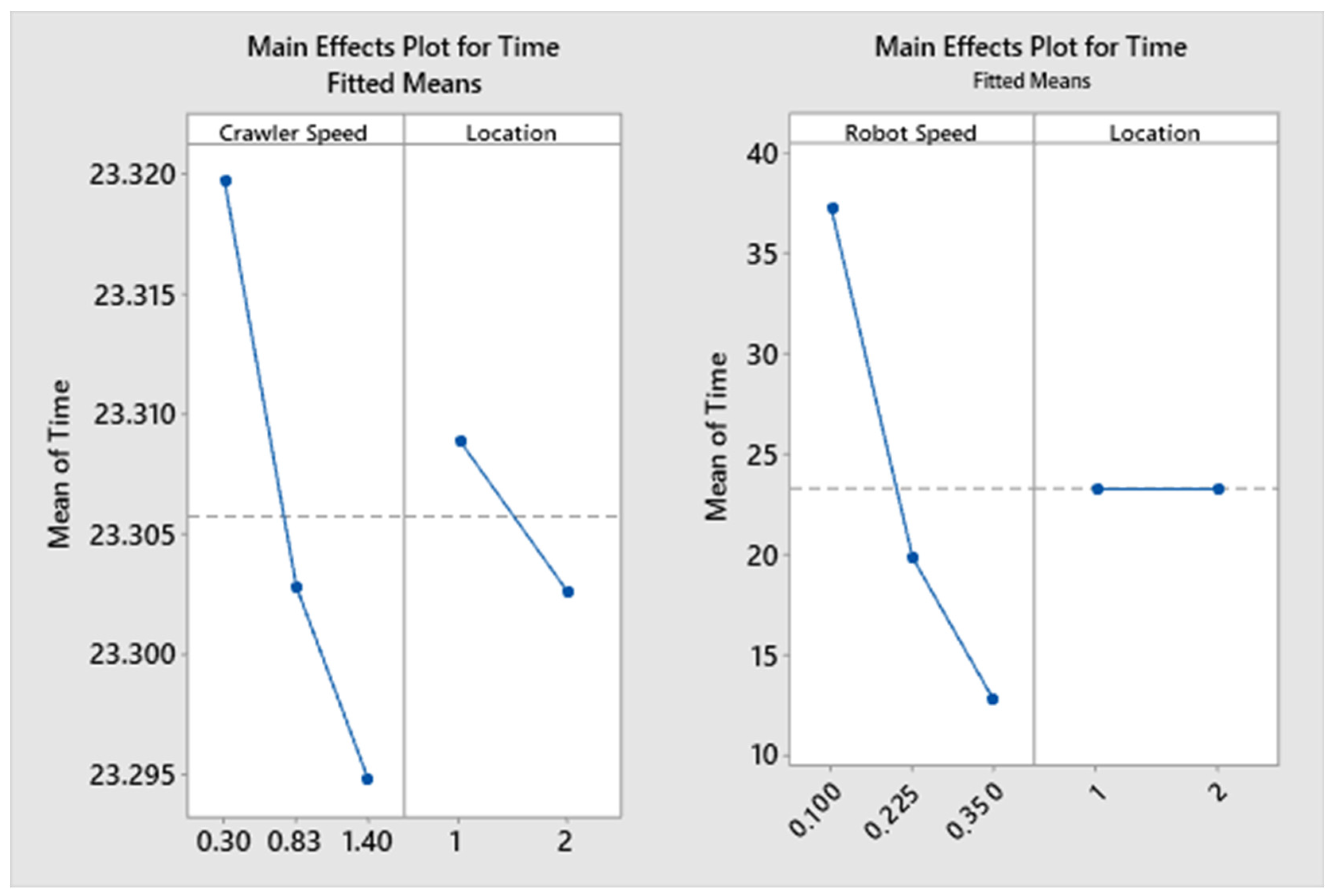
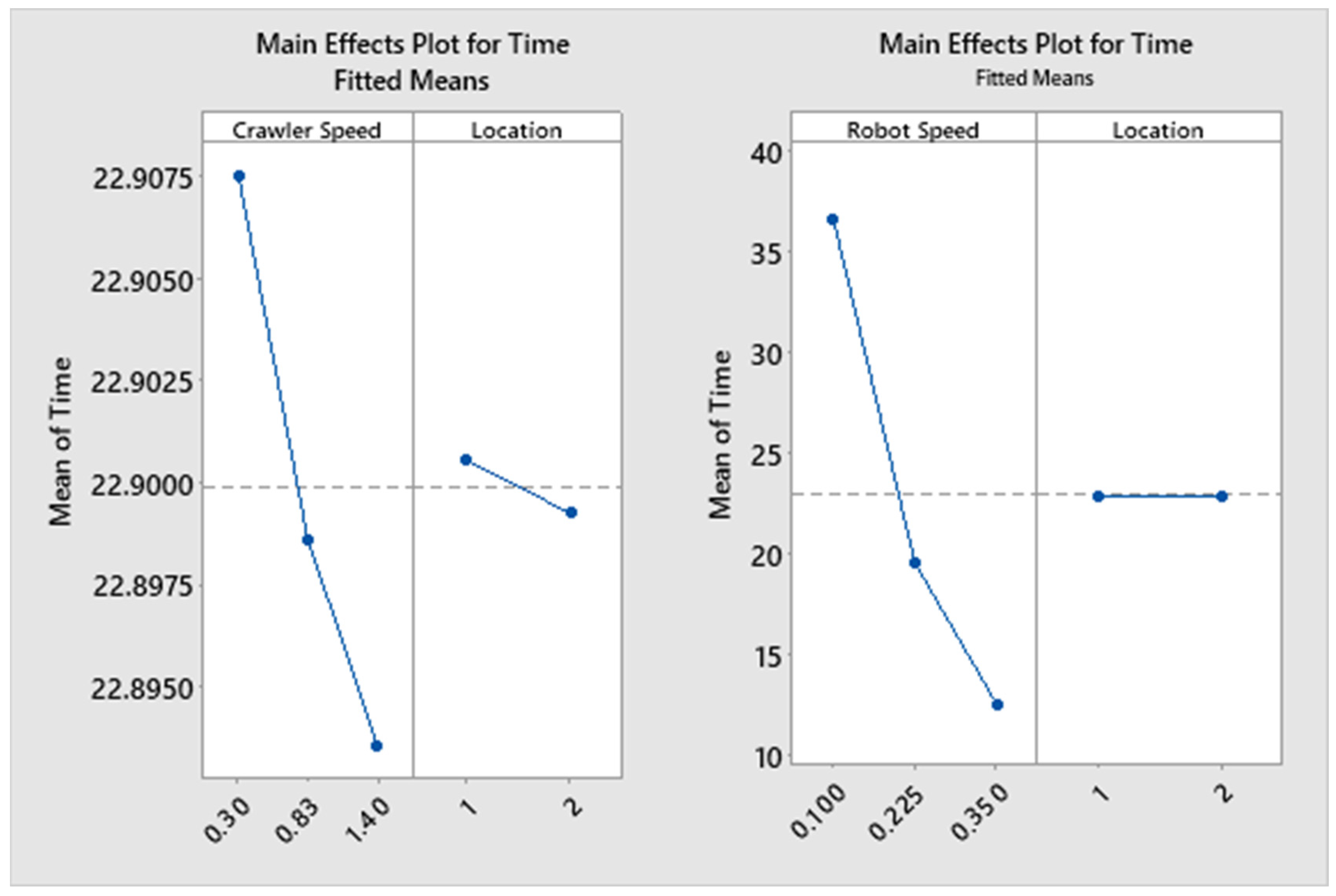
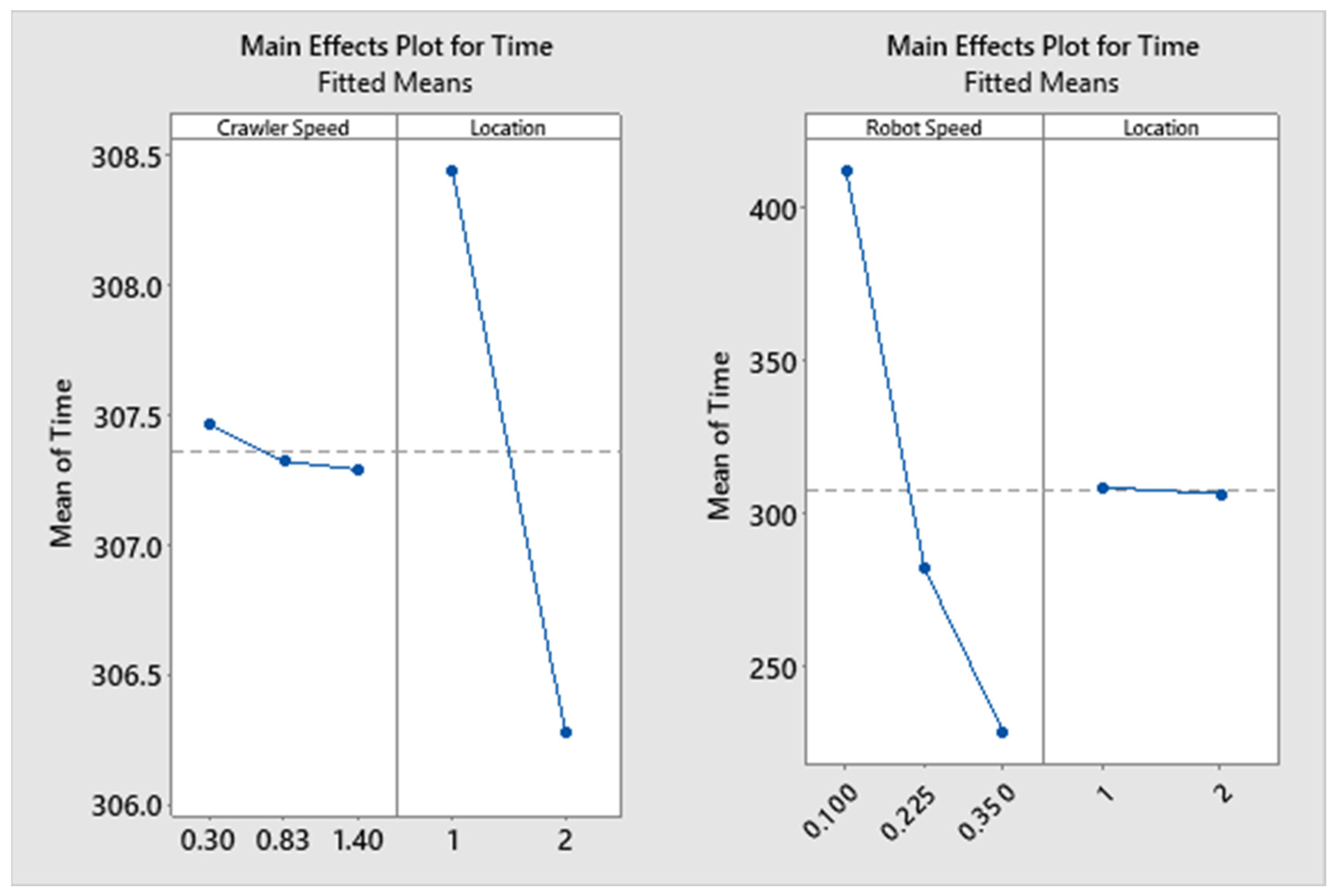
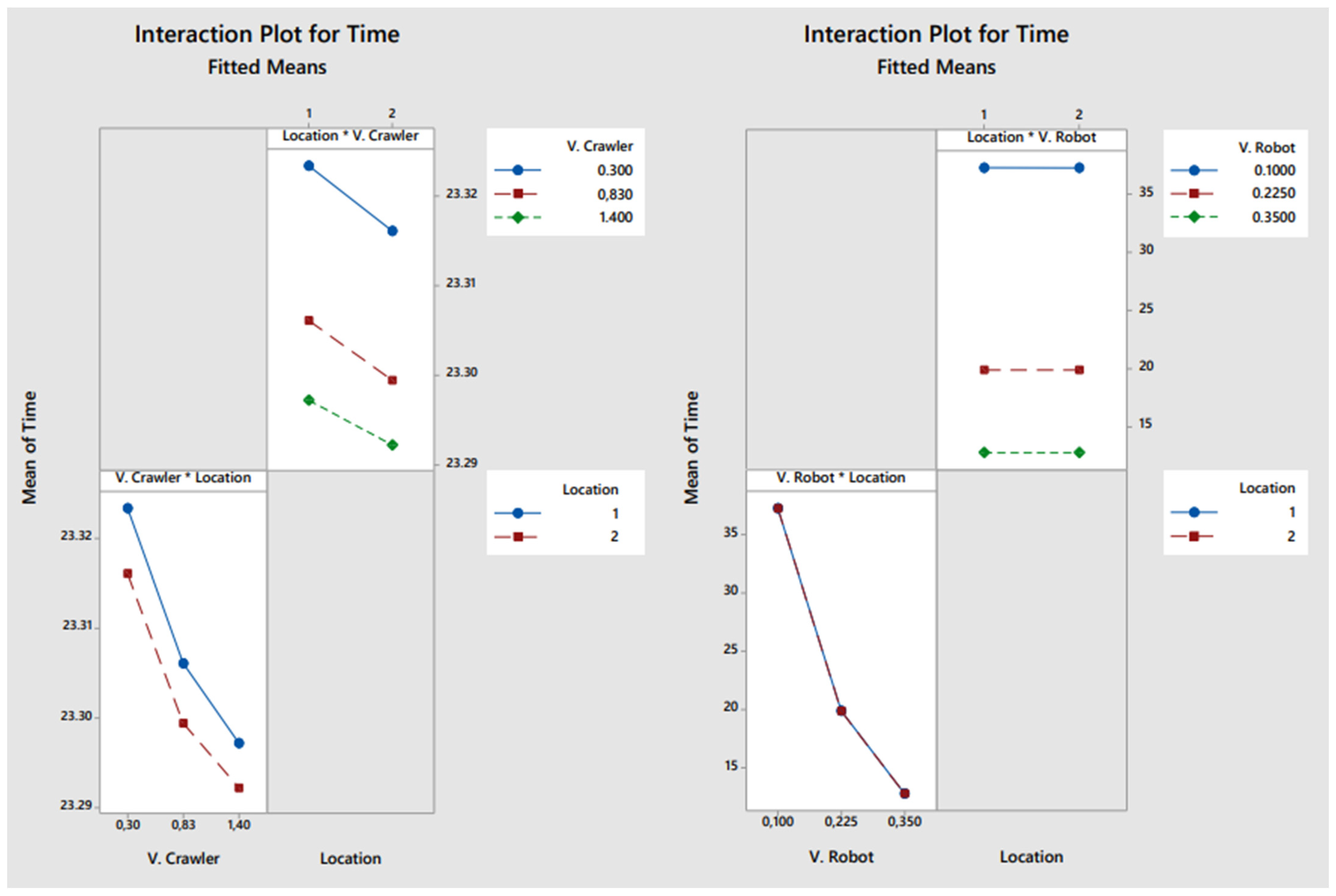
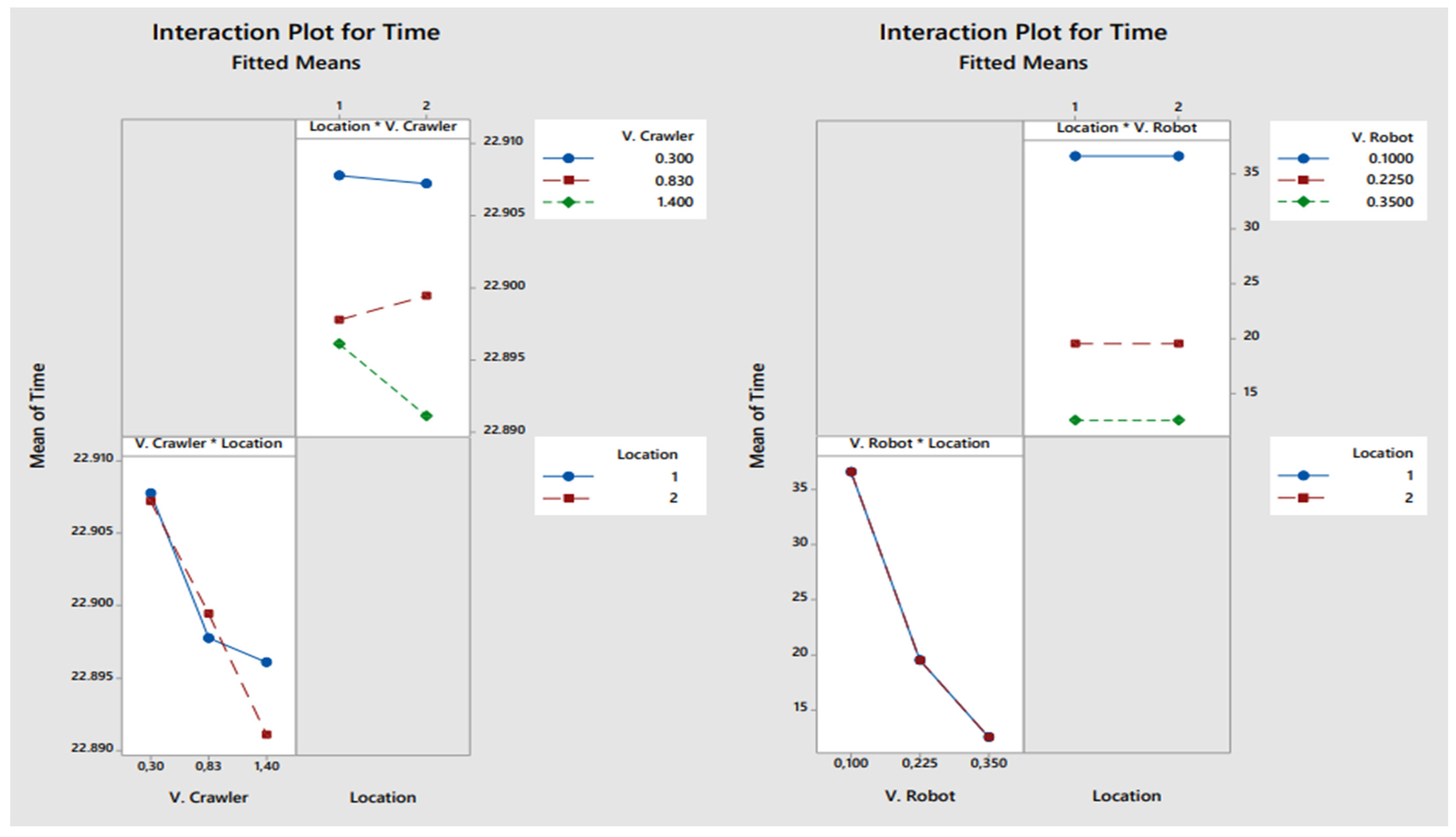
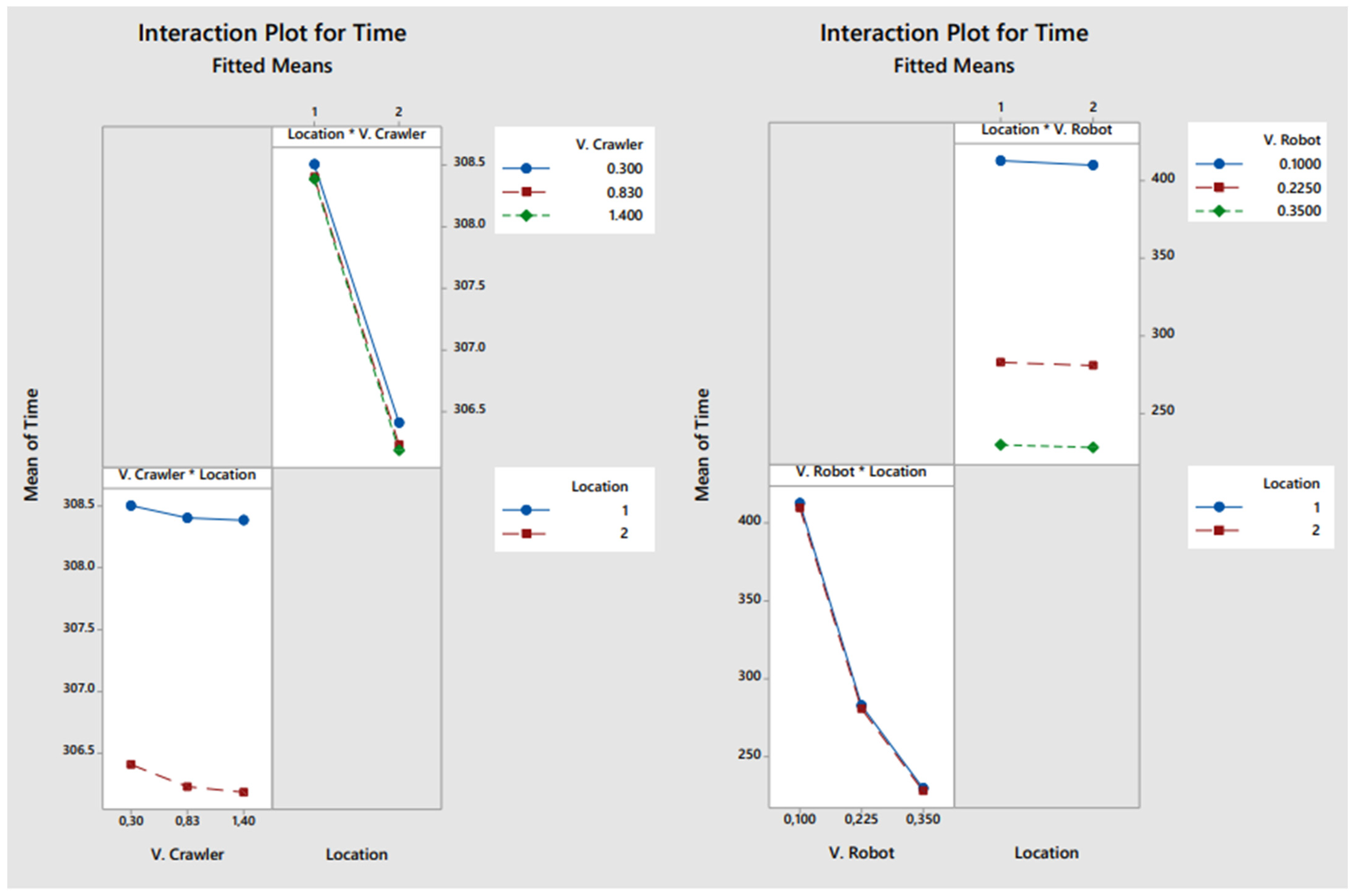
4.2.2.3. Graphs of the Factor Analyses

(a)

Main effect plots

Figure 14, Figure 15 and Figure 16 show the behavior of the variables, indicating to what extent they affect the different test levels. These graphs show the mean time for each factor level, and then these values are joined with a line to evaluate their behavior.

As shown on the right side of Figure 14 (floor 1 of the small building), in the area of factor A, the line is not horizontal, indicating a main effect and, therefore, that the different levels of this factor affect the response variable differently. For example, as the robot’s speed increases, the time decreases by 65.69%. However, the opposite case happens with the location since the line is almost horizontal, indicating that each level of factor C affects the time in practically the same way, so the location, in this case, is not the main effect. Then, in the left section, the line has a non-horizontal behavior for factor B, presenting a slight slope. This indicates that the three levels that take this variable affect the simulation time in different ways. Concerning the location, it can be seen that its two levels affect the time average, but its variation is not so significant. Likewise, the crawler having a higher displacement speed and working in the second location favor the drop-in time, but to a much lesser extent, since it presents a drop of 0.027% and 0.107%, respectively.

Later, Figure 15 (floor 2 of the small building) shows the same behavior as floor 1, where maximizing the speeds of the robot and the crawler leads to a decrease in time of 65.71% and 0.061%, respectively. In addition, when working with location 2, the duration decreases by 0.006%.

In the big building, according to Figure 16, the behavior of its peers is repeated. A negative effect is seen when changing from a low to a high level, decreasing the time by 44.344%, 0.056%, and 0.699% for the robot speed, crawler speed, and locations, respectively.

(b)

Interaction graphs

These interaction graphs show the impact of the factors on the response variable. It should be noted that the effect of a factor depends on the level of the other factor, so it is relevant to evaluate the interactions and thus know their behavior. These graphs show the interactions generated according to the robot speed, crawler speed, and locations with the time variable.

Figure 17 shows an interaction plot for time presented for the second floor of the small building. On the left at the bottom, for the crawler speed * location type chart, the average interaction time varies from higher to lower, according to the increase in the crawler speed.

It can be seen that they are non-parallel lines, indicating an interaction between them, and highlighting that the less parallel they are, the greater the interaction strength they will have.

When looking at the low level of the crawler speed for location type one, there is a higher mean time than the one obtained for location type two, thus indicating that location type two is the most convenient for the crawler vehicle.

When observing the right side at the bottom, we see the graph for robot speed ∗ location type. In this case, the average interaction time also goes from higher to lower as the robot’s speed increases. Furthermore, on this side of the graph, it is observed that the average time obtained for each factor level has the same value in locations one and two. Therefore, the robot in any of the two locations acts similarly, showing that the location type used by the robot does not influence the time spent in the simulation.

Finally, from this figure, it can be noted that the shortest time is achieved using the maximum speed of the robot, the maximum speed of the crawler, and the second type of location, thus minimizing the simulation time.

Figure 18 shows in the crawler speed ∗ location type interaction chart that the mean time decreases as the crawler speed increases. In addition, the behavior of the lines for the locations shows that these are slightly non-parallel lines, so their interaction strength is not as high. This interaction effect indicates that the relationship between the crawler speed and location depends on the value of the simulation time, since by using the minimum crawler speed and location 1, the highest mean time is associated with them. However, using the average speed of the crawler and location 2 is also associated with the highest mean time. The robot speed ∗ location type graph repeats the same as that for floor one. Therefore, the mean time obtained for each factor level has the same value in locations one and two. Thus, it is inferred that to minimize the simulation time, it is necessary to choose the configuration in which the robot speed is at a maximum, which is also the case in which the crawler and the second type of location are used.

In Figure 19, the interaction graph shows that for crawler speed ∗ location type, the average time decreases as the speed of the crawler increases. However, unlike the two previous cases, it does not present such a large slope when passing from one level to another. In addition, the lines for the locations indicate that they are slightly non-parallel lines, so their interaction strength is not so high. When using the minimum speed of the crawler, it can be seen that the highest mean time is associated with location 1. In contrast, location 2, for that same speed, has a lower mean time, showing that location 2 for the crawler is more convenient than location 1.

In the graph of robot speed ∗ location type, the behavior of its peers is repeated. Then, the average time for each level of the factor has the same value in locations 1 and 2. Therefore, to minimize the simulation time, the robot speed and the crawler should be at their maximum levels, and location 2 should be used.

4.2.2.4. Optimization of Simulation Time

Optimization of the response variable was performed to reduce the simulation time. Five combinations were tested, and the results are shown in Table 7, Table 8 and

Table 9. Optimal conjugations of variables to minimize simulation time in hours for the standard floor of the big building.

Solution	Robot Speed	Crawler Speed	Location Type	Time Fit	Composite Desirability
1	0.35	1.4	2	228.018	0.999955
2	0.35	0.83	2	228.067	0.999693
3	0.35	0.3	2	228.243	0.998737
4	0.35	1.4	1	229.677	0.990982
5	0.35	0.83	1	229.687	0.990928

.

In this way, the best configuration for floor 1 of the small building corresponds to using the maximum value for both speeds and location 2, obtaining a time of 12.77 hours. For floor 2, a minimum duration of 12.545 hours is achieved when using the highest speeds and location 2. Finally, for the big building, with maximum speeds and location 2, a minimum time of 228,018 hours was obtained.

4.3. Comparison between Conventional Construction Methodologies and AM

To compare these methodologies, the time required for the execution of a concrete wall was used. In the case of AM, the configurations from “Section 4.2.2.4. Optimization of simulation time” were used to obtain the time. For the traditional system, the information provided by Ruano [46], who estimated that to build a wall of 45.3 m³, including the fabrication and placement of reinforcement, the assembly and placement of formworks, and the pouring of concrete, in addition to considering the permanence of the formworks, 4.78 days are used. For a working day of 9 hours, 4.78 days correspond to 43.02 hours.

On the hand, the values found in “Section 4.2.2.4 Simulation time optimization” for the AM process are summarized in

Table 10. Construction time of buildings under study made using AM.

Variables	Small Building		Big Building
Floor	Floor 1	Floor 2	Standard floor
Time per floor	12.77 h	12.545 h	228.018 h
Total time	23.315 h		2736.216 h

, presenting the time required for the concrete extrusions of 48.84 m³ (Small building) and 2082.93 m³ (Big building).

As the time used in the traditional system is for a wall of 45.3 m³, this amount must be extrapolated to the volume to build the two buildings considered in this study to know the approximate duration when conventional construction is used, as shown in

Table 11. Time used to build the walls of the Small building in a conventional way.

Activity	Duration
Rebar fabrication	1.06 days
Rebar installation	0.95 days
Placement of wall formwork	1.87 days
Concrete pouring	0.20 days
Waiting time before removing formworks	1.00 days
Total duration	5.08 days

and

Table 12. Time used to build the walls of the Big building in a conventional way.

Activity	Duration
Rebar fabrication	45.27 days
Rebar installation	40.41 days
Placement of wall formwork	79.63 days
Concrete pouring	8.72 days
Waiting time before removing formworks	8.72 days
Total duration	182.74 days

. According to Table 11, using the conventional system for the small building gives a time of 5.08 days or 45.72 hours. On the other hand, as shown in Table 12, for the construction of the big building, 182.74 days or 1,645 hours were spent.

As a result, when comparing the time used in a conventional construction system for the construction of concrete walls and the maximum duration of 3D-printed walls obtained when configuring the mobile robot with its maximum extrusion speed, it is possible to demonstrate that this method is 45% faster than traditional construction for the small building. On the other hand, for the big building, there is a difference of 40% in favor of conventional construction in comparison with the 3DCP process for walls; however, we have to take into account that for the big building, only 1 robot was used to print the whole building. After running the same analysis but using 3 robots instead of 1, the total time for 3DCP (using the highest speed of the robot), was 912 hours or 101.33 days, i.e., 81.41 hours faster than the conventional system (more than 80% faster in favor of the 3DCP process).

4.4. Discussion

The methodology presented in this research has been shown to be a useful tool for easily simulating 3DCP processes for residential buildings. This may open up a wide range of opportunities for the construction sector since it is increasingly common to find more and more complex architectural geometries [13,14] that need to be first simulated before being built.

From a theoretical and methodological perspective, this research may contribute to the body of knowledge by providing a practical tool for computing the simulation of complex geometries to be printed in construction projects through DES, which may be implemented by construction professionals without any previous experience in simulation.

From the numerical analyses carried out, it was found that on floor 1 of the small building, the robot speed and the crawler speed significantly influenced the printing time, while on floor 2, the robot speed was the most influential. For the big building, the factor that had the most significant influence was the location. However, after running combined analyses, it was found that the robot speed was the most significant factor in all cases. Finally, the interaction analyses show that the shortest printing times are achieved when the robot speed and crawler speed are at a maximum and the second location is chosen.

5. Conclusions

Three-dimensional printing is increasingly important in the construction industry because of its versatility and speed when building different types of construction projects. With these advantages in mind, it is essential to know the protocols and procedures to simulate projects to provide an approximation of what can happen before construction begins. In this sense, this study focused on simulating the performance of a mobile robot that prints 3D concrete walls under different configurations. The most relevant variables that were considered were extrusion speed, crawler speed, and robot locations, generating different scenarios to estimate the real duration of the construction process.

The code that was developed through a process flow in FlexSim^TM is a simulation methodology that can be easily extrapolated to other construction projects by setting the locations of the “Queues”. Regarding the experimental design, the goodness-of-fit test served to investigate the probabilistic behavior that the simulation demonstrated in addition to delivering a mean value and standard deviation for each speed and location of the robot, showing that the times for the small building corresponded to a normal distribution and those of the big building to a log-normal distribution.

In terms of average completion times, the duration for the small building was 1.64 days and for the big building 141.41 days, where the most influential variable was the extrusion speed of the robot over the movement of the crawler or the location of the robot. This makes sense because most of the total time is devoted to the 3DCP process, whereas the speed of the crawler that moves the robot and its locations is less predominant. Therefore, the best configuration to minimize the construction times was obtained by using the maximum speed values and location 2 in all cases, which is deducible since the higher the speed, the shorter the time, with the location being a more unpredictable factor.

Regarding the comparison between the conventional construction system and AM, the latter was faster in the case of the small building, but the opposite occurred for the big building. However, we have to take into account that for the big building, only 1 robot was used (versus dozens of crews of workers involved, as is usual for large buildings), but when 3 simultaneous robots were considered, the 3DCP process was definitively much faster (80% to be precise).

As a limitation, it is important to mention that this study considered a combination of two locations (thinking about the best layout according to the configuration of the walls of each floor); however, in terms of future research lines, multiple positions could be added, which would require the use of multi-objective optimization methods as a complement to the simulation analysis presented in this study. On the other hand, also taking into account the continuation of this research in the future, although the printing simulation presented herein considered a probabilistic behavior to absorb part of the variability in the simulated processes, in practice, other real operating conditions of robot printing should be added, such as possible clogging in the concrete pump, delays in the provision of materials, and potential stoppages due to the biological needs of the pump operator, among other variables that could influence the performance obtained in this investigation. Furthermore, in terms of future studies, it could be interesting to make a comparison between geometric and organic shapes to analyze efficiency of the manufacturing process.

In summary, this study allowed presenting a simplified and replicable procedure to simulate 3DCP processes, considering the following variables: the speed of the robot that extrudes the concrete, the speed of the crawler system that transports the robot from one place to another, and the different positions to which it can take this robot. Of all these variables, the extrusion speed—in terms of the robot’s speed—was the most relevant. Finally, the present simulation process also allowed determining that for small-scale construction (a two-story house, i.e., the small building), one robot is significantly faster than a conventional construction process and that for larger-scale construction (with twelve floors, i.e., the big building), only three printing robots are enough to exceed the conventional construction times.

References

1. F2792-12A; ASTM International Standard Terminology for Additive Manufacturing Technologies. ASTM International: West Conshohocken, PA, USA, 2012.
2. Campillo Mejías, M. Prefabricación en la Arquitectura: Impresión 3D en Hormigón; Universidad Politécnica de Madrid: Madrid, Spain, 2017. [Google Scholar]
3. Nadal, A.; Pavón, J.; Liébana, Ó. Perspectivas para la impresión 3D en la construcción. Rev. Eur. Investig. Arquit. REIA 2017, 7–8, 231–244. [Google Scholar]
4. Shahrubudin, N.; Lee, T.C.; Ramlan, R. An Overview on 3D Printing Technology: Technological, Materials, and Applications. Procedia Manuf. 2019, 35, 1286–1296. [Google Scholar] [CrossRef]
5. Babalola, O.; Ibem, E.O.; Ezema, I.C. Implementation of lean practices in the construction industry: A systematic review. Build. Environ. 2019, 148, 34–43. [Google Scholar] [CrossRef]
6. Agustí-Juan, I.; Müller, F.; Hack, N.; Wangler, T.; Habert, G. Potential benefits of digital fabrication for complex structures: Environmental assessment of a robotically fabricated concrete wall. J. Clean. Prod. 2017, 154, 330–340. [Google Scholar] [CrossRef]
7. García, R.; Martínez, A.; González, L.; Auat, F. Projections of 3D-printed construction in Chile. Rev. Ing. Constr. 2020, 35, 60–72. [Google Scholar] [CrossRef]
8. ABB Robotics. Product Specification IRB 6700; ABB Ltd.: Zurich, Switzerland, 2021; p. 170. [Google Scholar]
9. CyBe Construction. CyBe 3Dcp Specifications; CyBe Construction: Oss, The Netherlands, 2022; pp. 1–16. [Google Scholar]
10. Forcael, E.; Pérez, J.; Vásquez, Á.; García-Alvarado, R.; Orozco, F.; Sepúlveda, J. Development of communication protocols between bim elements and 3D concrete printing. Appl. Sci. 2021, 11, 7226. [Google Scholar] [CrossRef]
11. du Plessis, A.; Babafemi, A.J.; Paul, S.C.; Panda, B.; Tran, J.P.; Broeckhoven, C. Biomimicry for 3D concrete printing: A review and perspective. Addit. Manuf. 2021, 38, 101823. [Google Scholar] [CrossRef]
12. Ooms, T.; Vantyghem, G.; Van Coile, R.; De Corte, W. A parametric modelling strategy for the numerical simulation of 3D concrete printing with complex geometries. Addit. Manuf. 2021, 38, 101743. [Google Scholar] [CrossRef]
13. Carneau, P.; Mesnil, R.; Roussel, N.; Baverel, O. Additive manufacturing of cantilever—From masonry to concrete 3D printing. Autom. Constr. 2020, 116, 103184. [Google Scholar] [CrossRef]
14. Prasittisopin, L.; Sakdanaraseth, T.; Horayangkura, V. Design and Construction Method of a 3D Concrete Printing Self-Supporting Curvilinear Pavilion. J. Archit. Eng. 2021, 27, 05021006. [Google Scholar] [CrossRef]
15. Forcael, E.; Ferrari, I.; Opazo-Vega, A.; Pulido-Arcas, J.A. Construction 4.0: A Literature Review. Sustainability 2020, 12, 9755. [Google Scholar] [CrossRef]
16. Maskuriy, R.; Selamat, A.; Maresova, P.; Krejcar, O.; David, O.O. Industry 4.0 for the construction industry: Review of management perspective. Economies 2019, 7, 68. [Google Scholar] [CrossRef]
17. Sawhney, A.; Riley, M.; Irizarry, J. Construction 4.0; Sawhney, A., Riley, M., Irizarry, J., Eds.; Routledge: London, UK, 2020; ISBN 9780429398100. [Google Scholar]
18. Bourell, D.L. Perspectives on Additive Manufacturing. Annu. Rev. Mater. Res. 2016, 46, 1–18. [Google Scholar] [CrossRef]
19. Sakin, M.; Kiroglu, Y.C. 3D Printing of Buildings: Construction of the Sustainable Houses of the Future by BIM. Energy Procedia 2017, 134, 702–711. [Google Scholar] [CrossRef]
20. Lopez, J. Fabricación aditiva y transformación logística: La impresión 3D. Oikonomics Rev. Econ. Empres. y Soc. 2018, 9, 58–69. [Google Scholar]
21. Christoph, R.; Muñoz, R.; Hernández, Á. Manufactura Aditiva. Real. y Reflexión 2017, 16, 97–109. [Google Scholar] [CrossRef]
22. Bos, F.; Wolfs, R.; Ahmed, Z.; Salet, T. Additive manufacturing of concrete in construction: Potentials and challenges of 3D concrete printing. Virtual Phys. Prototyp. 2016, 11, 209–225. [Google Scholar] [CrossRef]
23. Roselló, D. Estudio de Las Aplicaciones de la Impresión 3D en el Ámbito de la Construcción; Universidad Politécnica de Cataluña: Barcelona, Spain, 2022. [Google Scholar]
24. Davtalab, O.; Kazemian, A.; Khoshnevis, B. Perspectives on a BIM-integrated software platform for robotic construction through Contour Crafting. Autom. Constr. 2018, 89, 13–23. [Google Scholar] [CrossRef]
25. Law, A.; Kelton, D. Simulation Modeling and Analysis, 5th ed.; McGraw-Hill: New York, NY, USA, 2014; ISBN 978-0-07-340132-4. [Google Scholar]
26. Forcael, E.; González, M.; Soto-Muñoz, J.; Ramis, F.; Rodríguez, C. Simplified Scheduling of a Building Construction Process using Discrete Event Simulation. In Proceedings of the 16th LACCEI International Multi-Conference for Engineering, Education, and Technology: “Innovation in Education and; Inclusion”, Lima, Peru, 19–21 July 2018. [Google Scholar]
27. Páez, H.J. Simulación Digital Para el Mejoramiento de la Planeación de Procesos Constructivos; Universidad de Los Andes: Bogotá, Colombia, 2007. [Google Scholar]
28. Abdelmegid, M.A.; González, V.A.; Poshdar, M.; O’Sullivan, M.; Walker, C.G.; Ying, F. Barriers to adopting simulation modelling in construction industry. Autom. Constr. 2020, 111, 103046. [Google Scholar] [CrossRef]
29. Ramón, A.; Barboza, R. Uso de la simulación en procesos de construcción. Rev. Tecnol. Marcha 2019, 32, 145–157. [Google Scholar] [CrossRef]
30. Gómez, A. Simulation of constructive processes. Rev. Ing. Constr. 2010, 25, 121–144. [Google Scholar] [CrossRef]
31. Kamat, V.R.; Martinez, J.C. Visualizing Simulated Construction Operations in 3D. J. Comput. Civ. Eng. 2001, 15, 329–337. [Google Scholar] [CrossRef]
32. González, V.; Alarcón, L. Buffers de programación: Una estrategia complementaria para reducir la variabilidad en los procesos de construcción. Rev. Ing. Construcción 2003, 18, 109–119. [Google Scholar]
33. Singh, P.M.; Singari, R.; Mishra, R.S. A review of study on modeling and simulation of additive manufacturing processes. Mater. Today Proc. 2022, 56, 3594–3603. [Google Scholar] [CrossRef]
34. Mostafaei, A.; Elliott, A.M.; Barnes, J.E.; Li, F.; Tan, W.; Cramer, C.L.; Nandwana, P.; Chmielus, M. Binder jet 3D printing—Process parameters, materials, properties, modeling, and challenges. Prog. Mater. Sci. 2021, 119, 100707. [Google Scholar] [CrossRef]
35. Ninpetch, P.; Kowitwarangkul, P.; Mahathanabodee, S.; Chalermkarnnon, P.; Ratanadecho, P. A review of computer simulations of metal 3D printing. In Proceedings of the AIP Conference Proceedings, Pattaya, Thailand, 11–13 September 2020; AIP Publishing: Pattaya, Thailand, 2020; p. 050002. [Google Scholar]
36. Zhang, G.Q.; Spaak, A.; Martinez, C.; Lasko, D.T.; Zhang, B.; Fuhlbrigge, T.A. Robotic additive manufacturing process simulation–towards design and analysis with building parameter in consideration. In Proceedings of the 2016 IEEE International Conference on Automation Science and Engineering (CASE), Fort Worth, TX, USA, 21–25 August 2016; pp. 609–613. [Google Scholar]
37. Paolini, A.; Kollmannsberger, S.; Rank, E. Additive manufacturing in construction: A review on processes, applications, and digital planning methods. Addit. Manuf. 2019, 30, 100894. [Google Scholar] [CrossRef]
38. Lei, Z.; Han, S.; Bouferguène, A.; Taghaddos, H.; Hermann, U.; Al-Hussein, M. Algorithm for Mobile Crane Walking Path Planning in Congested Industrial Plants. J. Constr. Eng. Manag. 2015, 141, 05014016. [Google Scholar] [CrossRef]
39. Valdivieso, C. Europe’s First 3D Concrete Printing Facility. 3D Natives. 2019. Available online: https://www.3dnatives.com/en/3d-concrete-printing-facility-230120195/ (accessed on 1 March 2023).
40. Bouygues, C. The Future of 3D Printing in Construction—Interview with Bruno Linéatte, Director of R&D for Building Construction Methods at Bouygues Construction; Bouygues Construction: Guyancourt, France, 2020; Available online: https://www.bouygues-construction.com/blog/en/impression-3d-construction/ (accessed on 1 March 2023).
41. CIPYCS (Centro Interdisciplinario para la Productividad y Construcción Sustentable). Prototipado a Escala Piloto. 2020. Available online: https://construye2025.cl/2020/08/28/laboratorio-de-infraestructura-modular-alista-operaciones-para-junio-de-2021/ (accessed on 1 March 2023).
42. Saunders, S. CyBe Construction Unveils New Mobile 3D Concrete Printer, the CyBe RC 3Dp. 2016. Available online: https://3dprint.com/158972/cybe-mobile-3d-concrete-printer/ (accessed on 1 March 2023).
43. Back, W.E.; Boles, W.W.; Fry, G.T. Defining Triangular Probability Distributions from Historical Cost Data. J. Constr. Eng. Manag. 2000, 126, 29–37. [Google Scholar] [CrossRef]
44. Kamiński, M. Uncertainty analysis in solid mechanics with uniform and triangular distributions using stochastic perturbation-based Finite Element Method. Finite Elem. Anal. Des. 2022, 200, 103648. [Google Scholar] [CrossRef]
45. Giftthaler, M.; Sandy, T.; Dörfler, K.; Brooks, I.; Buckingham, M.; Rey, G.; Kohler, M.; Gramazio, F.; Buchli, J. Mobile robotic fabrication at 1:1 scale: The In situ Fabricator. Constr. Robot. 2017, 1, 3–14. [Google Scholar] [CrossRef]
46. Ruano, V. Análisis de Los Plazos de Construcción de Edificios en Chile y su Relación con Los Métodos Constructivos Utilizados. Bachelor’s Thesis, University of Chile, Santiago, Chile, 2010; pp. 1–126. [Google Scholar]
Figure 1. Small building: (a) first-floor simulation; (b) second-floor simulation; and (c) final model.
Buildings 13 01390 g001
Figure 2. Big building. (a) Simulation of the standard floor; (b) final model.
Buildings 13 01390 g002
Figure 3. Robot working range and dimensions (measurements in mm).
Buildings 13 01390 g003
Figure 4. Robot base and tracked vehicle dimensions (measurements in mm).
Buildings 13 01390 g004
Figure 5. EOAT examples added to a robotic arm: (a) ABB, (b) CyBe, and (c) Kuka (adapted from [39,40,41]).
Buildings 13 01390 g005
Figure 6. (a) Side view of robot’s reach (mm); (b) ABB robot on tracked CyBe vehicle (adapted from [42]).
Buildings 13 01390 g006
Figure 7. Maximum and minimum operation ranges of the robot (in mm).
Buildings 13 01390 g007
Figure 8. Flow diagram of the simulation process.
Buildings 13 01390 g008
Figure 9. Type of configuration analysis for the small building: (a) S11, (b) S12; (c) S21; and (d) S22 (blue arrows show the direction in which the robot moves on crawler; red circles show the operating radius of the robot in each position, and blue numbers show the different positions of the robot).
Buildings 13 01390 g009
Figure 10. FlexSimTM modeling of the printing sequence for analysis type S11 (green arrows are the directions where the robot moves, and black squares are the multiple robot locations).
Buildings 13 01390 g010
Figure 11. Locations for the analysis type B12 for exterior walls (a) and interior walls (b) (blue arrows show the direction in which the robot moves on crawler; red circles show the operating radius of the robot in each position, and blue numbers show the different positions of the robot).
Buildings 13 01390 g011
Figure 12. Printing sequence for analysis type B12 (green arrows are the directions where the robot moves, and black squares are the multiple robot locations).
Buildings 13 01390 g012
Figure 13. Pareto charts of standardized effects for (a) floor 1—small bldg.; (b) floor 2—small bldg.; and (c) standard floor—big bldg.
Buildings 13 01390 g013
Figure 14. The plot of main effects versus time for floor 1 of the small building.
Buildings 13 01390 g014
Figure 15. The plot of main effects versus time for floor 2 of the small building.
Buildings 13 01390 g015
Figure 16. The plot of main effects versus time for the standard floor of the big building.
Buildings 13 01390 g016
Figure 17. Interaction graph of variables concerning time for floor 1 of the small building.
Buildings 13 01390 g017
Figure 18. Interaction graph of variables concerning time for floor 2 of the small building.
Buildings 13 01390 g018
Figure 19. Interaction graph of variables concerning time for the standard floor of the big building.
Buildings 13 01390 g019