Abstract
With the development of various metaheuristic algorithms, research cases that perform weight optimization of truss structures are steadily progressing. In particular, due to the possibility of developing quantum computers, metaheuristic algorithms combined with quantum computation are being developed. In this paper, the QbHS (Quantum based Harmony Search) algorithm was proposed by combining quantum computation and the conventional HS (Harmony Search) algorithms, and the size and topology optimization of the truss structure was performed. The QbHS algorithm has the same repetitive computational structure as the conventional HS algorithm. However, the QbHS algorithm constructed (Quantum Harmony Memory) using the probability of Q-bit and proposed to perform pitch adjusting using the basic state of Q-bit. To perform weight optimization of truss structures using the proposed QbHS algorithm, 20 bar, 24 bar, and 72-bar truss structures were adopted as examples and compared with the results of the QE (Quantum Evolutionary) algorithm. As a result, it was confirmed that the QbHS algorithm had excellent convergence performance by finding a lower weight than the QE algorithm. In addition, by expressing the weight optimization results of the truss structure with an image coordinate system, the topology of the truss structure could be confirmed only by the picture. The results of this study are expected to play an important role in future computer information systems by combining quantum computation and conventional HS algorithms.
1. Introduction
Truss structures are widely applied to modern buildings because they can reduce the weight of the structure and are light. The optimal weight design to reduce the construction cost of truss structures and maximize the performance of members is of great interest to many researchers []. Weight optimal design is divided into size, shape, and topology optimization according to the method of selecting design variables. Size optimization selects the cross-sectional size of the member as the design variable and shape optimization selects the displacement of the joint of the structure as the design variable. Finally, topology optimization selects the presence or absence of each member or node as a design variable. Weight optimization, which was carried out by selecting one design variable, began to be studied as a combination of design variables such as size and shape, size and phase due to the development of computers.
Weight optimization of truss structures aims to find the minimum weight under various constraints. In general, the stress of the truss member, displacement of the node, and buckling stress of the member were widely used as constraints. However, the dynamic characteristics of the structure became important, and with the development of engineering, the natural frequency of the structure began to be added as a constraint. All structures have their frequency, and if the natural frequency and the frequency by dynamic load match, the horizontal displacement is amplified by the resonance phenomenon, posing a great risk to the safety and residence of the structure. Therefore, to prevent major damage caused by resonance phenomena, the natural frequency of the structure must be identified at the design stage [].
Weight optimization, a combination of size and topology, is widely applied to the optimal design of structures because it selects the optimal member size in the best topology. The combination problem of size and phase of truss structures was first performed by Sved and Ginos []. They used a 3-bar truss structure as an example, and only the stress of the member and the displacement of the joint were used as constraints. Since then, weight optimization of 9 bar, 10 bar, 22 bar, 28 bar, 37 bar, and 2415-bar truss structures has been performed by Sheu et al. and Ringertz [,,]. Nakamura et al. raised the need to add natural frequencies to constraints to the weight optimization problem of a combination of size and topology, and performed weight optimization of a 36-bar truss structure and an arch structure consisting of 55 nodes under only natural frequencies []. Since then, the weight optimization of the truss structure has been steadily carried out by many researchers, but most of the natural frequencies have not been included as constraint controls [,,,,,,,,]. Xu et al., Savsani et al. performed weight optimization of 10 bar, 20 bar, 24 bar, and 72-bar truss structures using all four constraints [,,].
Many researchers perform using metaheuristic algorithms for the optimal design of various engineering problems. The metaheuristics algorithm is an algorithm that mathematically describes natural phenomena and performs optimization, and typically includes GA (Genetic Algorithm), SA (Simulated Annealing), PSO (Particle Swarm Optimization), and TLBO (Teaching-Learning-Based Optimization) algorithms [,,,]. These metaheuristics algorithms are being combined with quantum computation to create new fields. Unlike Bit, which is expressed as ‘0’ or ‘1’, quantum computation uses Q-bit, which is expressed as the probability that ‘0’ and ‘1’ are selected [,]. Unlike conventional algorithms that are determined and derived from a single value, optimization using Q-bit can obtain a probability through information accumulation of Q-bit, and the probability of Q-bit is determined as a value through measurement []. In addition, it is possible to propose a new termination condition by accumulating information on Q-bit []. Due to these characteristics, many metaheuristic algorithms are combined with quantum computing, and algorithms such as Q-GA (Quantum GA), Q-PSO (Quantum PSO), Q-SA (Quantum SA), and Q-TLBO (Quantum TLBO) algorithms are proposed, and applied to various optimization problems [].
There have also been attempts to combine the HS (Harmony Search) algorithm proposed by Geem et al. with quantum computation. The problem of binary form, a basic study for combining HS algorithms that perform operations based on decimal numbers with quantum computation, has steadily progressed. Geem proposed a BHS (Binary HS) algorithm that can solve the On/Off switch problem []. Wang et al. proposed a hybrid BHS algorithm by applying the search mechanism of the ant system []. However, since the BHS algorithm was not easy to express the pitch adjusting process performed using values in the range of ‘0’ and ‘1’, the most important pitch adjusting process in the HS algorithm was omitted. Layeb proposed the QIHSA (Quantum Inspired HS Algorithm) that combines quantum computation and HS algorithms to solve the binary problem [], and Alfailakawi et al. attempted to express quantum gates as two-dimensional quantum circuits []. However, QIHSA can only solve problems expressed as ‘0’ or ‘1’, and algorithms that can solve real or binary variable problems are insufficient.
Therefore, this paper proposes a QbHS (Quantum based HS) algorithm that can solve real variable problems by combining the conventional HS algorithm with quantum computers. In addition, weight optimization of 20 bar, 24 bar, and 72-bar truss structures with continuous cross-sectional areas is performed using the QbHS algorithm and compared with the results of the QE (Quantum Evolutionary) algorithm. Section 2 describes the conventional HS algorithm, and Section 3 describes the overall theory of quantum computation and the QbHS algorithm. Section 4 defines the weight optimization problem of 20 bar, 24 bar, and 72-bar truss structures, and Section 5 shows the results of weight optimization. The final section concludes this paper.
2. The Conventional HS Algorithm
The conventional HS algorithm is an algorithm proposed by Geem et al. and is an algorithm that performs optimization by describing the process of finding the notes generated from the instrument in the best harmony []. The performers remember the notes they made and pitch adjusting to find the optimal harmony. (Harmony Memory) is the memory that remembers previously issued notes, and the size of is determined by N (number of instruments) and (Harmony Memory Size). The magnitude of the note adjustable width is (band-width). The variable considered for extraction from for pitch adjusting is (Harmony Memory Considering Rate), which has a value between ‘0’ and ‘1’. The variable considered for the extracted note regulation is (Pitch Adjusting Rate), which allows fine-tuning of the note depending on the width of . A small width of allows fine-tuning, which improves the convergence performance but slows the convergence. Conversely, the larger the width of , the faster the convergence rate, but the lower the convergence performance.
Algorithm 1 is a procedure for finding the best harmony in conventional HS algorithms and is divided into five steps.
| Algorithm 1 Process of conventional HS algorithm |
| Step 1: Define a problem and set HS parameters. |
| Step 2: Generate and initialize the memory. |
| Step 3: Create an new harmony by extracting one from and pitch adjusting. |
| Step 4: Update/renewal by using candidate harmony set. |
| Step 5: Repeat steps 3 and 4 until the stopping rules are satisfied. |
Step 1. Define a problem and set HS parameters
In Step 1, the optimization problem is defined and the value of the parameter is determined. The optimization problem can be defined as Equation (1).
Here, means the note generated by the i instrument, and and are the lower and upper limits of the problem. In addition, parameters that significantly affect the convergence performance of the conventional HS algorithms: , , , , (total generations) is set. In general, and are known to use 0.7–0.95 and 0.1–0.5 [].
Step 2. Generate and initialize the memory
The expression used to generate the note initially is Equation (2), and each note is stored in , such as Equation (3).
Here, , and is a random number between ‘0’ and ‘1’. That is, the conventional HS algorithm consists of in decimal variables.
Step 3. Create an new harmony by extracting one from and pitch adjusting
Step 3 is the step of generating a new note (), and is the most important step in conventional HS algorithms. is generated using , , and , and uses a value of by Equation (4). We take advantage of the value of if is less than or equal to , and if is greater than , it is globally explored by Equation (2). is a random number between ‘0’ and ‘1’.
The adopted by is determined by , according to whether pitch adjusting is performed. If is less than or equal to , pitch adjusting is performed by Equation (5), and if is greater than , it is globally explored by Equation (2). is a random number between ‘−1’ and ‘1’.
Step 4. Update/Renewal by using candidate harmony set
In Step 4, we compare solutions of notes () belonging to the existing with new solutions of notes () to update the better notes to . This process is expressed in an equation as Equation (5).
Step 5. Repeat steps 3 and 4 until the stopping rules are satisfied
If the t (current generation) is equal to the t set initially, the search is terminated, and if it is not equal, go to Step 3 and repeat until the end condition is satisfied.
3. Background of Quantum Computation
3.1. Expression of Q-Bit
Classical computers (including super-computers) calculate bits expressed as ‘0’ or ‘1’ as the minimum information processing unit, but quantum computers and quantum computations calculate using Q-bits that express values by overlapping ‘0’ and ‘1’. Bra-ket notification is used to express Q-bit, and the state of a single Q-bit is expressed as Equation (7) [].
and are probability amplitudes of |0> and |1>, and and are probabilities that |0> and |1> are chosen []. Since the sum of the probabilities must satisfy ‘1’, the sum of each probability must always satisfy Equation (8), which is called the normalized Q-bit. If the state of a single Q-bit is expressed as a vector matrix, it can be expressed as Equation (9).
If the number of Q-bits is m, the state of m Q-bits can be expressed as a vector matrix as shown in Equation (10). The sum of the probabilities that |0> and |1> of each Q-bit will be selected must likewise satisfy 1, which can be expressed as Equation (11). Here, .
Rotation Gate
Quantum operators have been proposed to simulate the spin phenomenon of Q-bit. Unlike classical logic gates, it has the characteristic of being reversible. To represent a quantum operator, it must be represented as a unitary transformation matrix, which can be represented as Equation (12) [].
The Q-bit accumulates information about the previous generation based on the current generation and performs rotation for information accumulation. The i-th Q-bit in the t-generation rotates using Equation (13).
Here, means the rotation angle for the Q-bit to rotate, and is defined by Equation (14). is determined by a lookup-table such as Table 1. Here, x denotes a binary string in the current generation, and b denotes an optimal binary string in the previous generation. is a variable initially determined by , and is defined as Equation (15). is a parameter defined by the user.

Table 1.
Look-up table for quantum rotation gate.
3.2. Gate
gate helps to actively escape if the solutions of the converged Q-bit fall into the local optimal solution. The Q-bit fully converges to ‘0’ or ‘1’ as the number of generations progresses, and the Q-bit is observed to show one solution. However, there is no way to escape through observation when the Q-bit falls into the local optimal solution with 100% convergence to ‘0’ or ‘1’. To solve this problem, Han et al. proposed gate [].
Figure 1 is the concept of gate, and the basic state of a single Q-bit is expressed in and axes. Han et al. [] classified it into three cases, and each case is expressed as an equation, namely as Equations (16)–(18). Case 1 and Case 2 beyond the range of are readjusted to , and Case 3 within the range of has the same value.
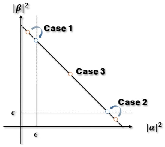
Figure 1.
Concept of gate.
That is, gate artificially prevents the phenomenon of full convergence to ‘0’ or ‘1’ by the size of the variable . has a value in the range of [0 1], and if becomes too large, there is no space for Q-bits to converge, resulting in poor convergence performance [].
4. Quantum Based HS Algorithm
The QbHS algorithm performs operations using Q-gate and Q-bit with uncertain and overlapping characteristics. The QbHS algorithm performs repetitive operations with basically the same structure as the conventional HS algorithm. Algorithm 2 is a procedure for performing the QbHS algorithm and is classified into five steps like the conventional HS algorithm.
| Algorithm 2 Process of QbHS Algorithm |
| Step 1: Define a problem and set QbHS parameters. |
| Step 2: Generate and initialize the memory. |
| Step 3: Create an new harmony by extracting one from and pitch adjusting. |
| Step 4: Update/renewal by using candidate harmony set. |
| Step 5: Repeat steps 3 and 4 until the stopping rules are satisfied. |
Step 1. Define a problem and set QbHS parameters
Like the conventional HS algorithm, the problem is defined in Step 1 and the parameters used in the QbHS algorithm are set. Like conventional HS algorithms, there are parameters (Quantum ), (Quantum ), (Quantum ), (Quantum ), and , with and is added. is used for the rotation gate for the rotation of Q-bit, and is the variable used for the gate.
Step 2. Generate and initialize the memory
The (Quantum ) of the QbHS algorithm has the same structure as the conventional HS algorithm and can be expressed as Equation (19).
of the conventional HS algorithm consists of a decimal variable, but consists of a binary variable represented by the measurement of Q-bit. Each variable can be expressed as Equation (20), where m represents the number of Q-bits per design variable.
Q-bit, which operates using probabilities, must determine the initial probability. In this paper, it was classified into two categories (QbHS or QbHS algorithm) using the method of initializing Q-bit. The QbHS algorithm initializes the probability of selecting ‘0’ or ‘1’ to 50% each. The QbHS algorithm initializes the probability of selecting ‘0’ or ‘1’ by generating random numbers between [0 1]. The probability of the initialized Q-bit is readjusted by gate. The Q-bit initialized using the above method is stored in the , and the determined stores information through measurement.
Step 3. Create a new harmony by extracting one from and pitch adjusting
After completing the initialization of , repetitive operations are performed using the same structure as the conventional HS algorithm. In the conventional HS algorithm, pitch adjusting is performed in Step 3, and it is the most important step in the calculation process. The QbHS algorithm performs pitch adjusting similarly, and unlike previous studies that omitted pitch adjusting because it was expressed in binary, this paper performs pitch adjusting using the basic state of Q-bit. Figure 2 is a diagram expressing the concept of pitch adjusting of the QbHS algorithm.
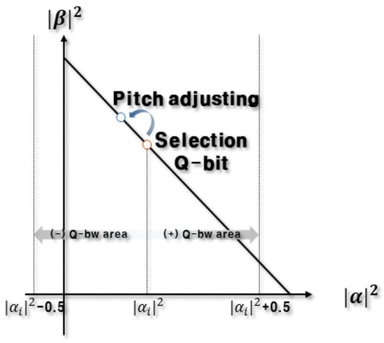
Figure 2.
Concept of pitch adjusting using Q-bit basic state.
Pitch adjusting is performed stochastically in the (+) or (−) direction using Q-bit’s probability information, and the range in which pitch adjusting is performed is [−0.5 0.5] based on the adopted Q-bit’s probability information . The process of performing pitch adjusting based on is expressed as an Equation (21). Here, r is a random number between ‘0’ and ‘1’, and is expressed as an Equation (22). Therefore, the size of gradually decreases as the number of generations progresses, and is determined by in which pitch adjusting is performed.
The Q-bits adopted for pitch adjusting are regulated by and . Figure 3 shows the Q-bit adopted according to the number of generations and is a figure with Q-bit, , and set to 10, 0.95, and 0.3. Pitch adjusting of the Q-bit performs probabilistically over the entire region until the probability mean of the Q-bit reaches . However, when the probability means reaches , pitch adjusting is performed using only Q-bits as much as . These changes in Q-bit adoption help the entire area of exploration in the early generation and conduct the role of exploitation in the latter generation.
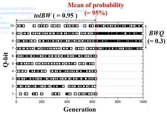
Figure 3.
Adaption of Q-bit in all generation.
After pitch adjusting is performed, it is readjusted by gate. If the conditions of and are not met, we randomly generate new information without performing pitch adjusting. The Q-bit of performs rotation on the previous generation based on the current generation and uses a rotation gate.
Step 4. Update/renewal by using candidate harmony set (Figure 4)
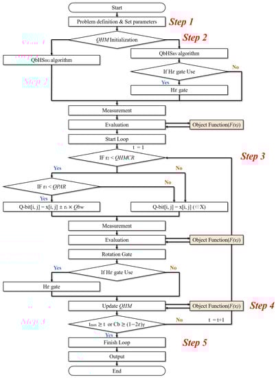
Figure 4.
Flowchart of QbHS algorithm.
The QbHS algorithm performs operations based on uncertainty data and is also stored in as information in Q-bit. Therefore, the renewal process of is determined by the measurement of of the current population and the candidate population. As a result of the measurement, the Q-bit passes through the rotation gate, and the probability information of the Q-bit is updated again. As the number of generations increases, the Q-bit converges to ‘0’ or ‘1’, resembling a state of definitive information. Through this process, the probability average of the Q-bit can be known indirectly. It can also recognize how current information has been accumulated.
Step 5. Repeat steps 3 and 4 until the stopping rules are satisfied
Like the conventional HS algorithm, if the t is the same as the , the search process is terminated. However, if the termination condition is not satisfied, move to Step 3 and perform a repetitive operation until the termination condition is met.
5. Problem Definition
The QbHS algorithm was applied to the weight optimization problem of truss structures, and the example structures adopted 20 bar, 24 bar, and 72-bar truss structures. Expressing the weight optimization problem as a mathematical model is equivalent to Equation (25) [,,].
Here, n is the number of elements, m is the number of nodes, is the density, is the cross-sectional area, is the length, is the mass of j nodes, is the stress, is the displacement of j nodes, is the critical buckling, is the Modules of elasticity, is the rth natural frequency of the truss. In this paper, for calculating buckling loads used 4.0, and 5.0 kg of mass was added to each node for calculating the natural frequency. is a topological bit, where ‘0’ means absent of the ith element, and ‘1’ means present of the ith element [].
The constraint checks the validity of the structure by checking whether the node that should not be erased, such as the node where the load is applied or the node set as the boundary, has been erased. If the constraint is not satisfied, the penalty is given by [].
The constraint identifies the kinematic stability of the structure and uses two steps. In the first step, the degree of freedom is calculated using Equation (27).
Here, d = 2 (for planar truss) or 3 (for space truss), and is a limited number of degrees of freedom. If is negative, it is determined that there is no mechanism. If is positive, it is determined that there is a mechanism, and penalties are given by . The second step checks the singularity of the global stiffness matrix (K). If eig(K) is greater than , it is judged that it is kinematically stable, and if it is less than , it is given a penalty of . Penalty values used in the paper were referred to the reference [,].
Unpenalized structures identify constraints , , , and , and, if all are satisfied, calculate the weight of the structures by Equation (25). If the constraints , , , and are not satisfied, a penalty is given by , which is equivalent to Equation (28).
Figure 5 is the initial shape of the truss structure adopted as an example. 20-bar truss structure in Figure 5a consists of 9 nodes and 20 elements, and an additional load of 200 kg was applied to the 4th node. 24-bar truss structure in Figure 5b consists of 8 nodes and 24 elements, and an additional load of 500 kg was applied to the third node. 72-bar truss structure in Figure 5c consists of 20 nodes and 72 elements, and an additional load of 2270 kg was applied to the first to fourth nodes. Truss structures of 20 bars and 24 bars have design variables equal to the number of elements. However, the 72-bar truss structure consists of 16 groups and has 16 variables: ( ), ( ), ( ), ( ), ( ), ( ), ( ), ( ), ( ), ( ), ( ), ( ), ( ), ( ), ( ), ( ).
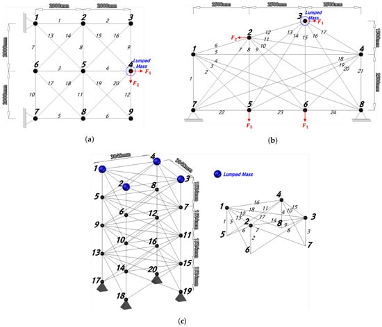
Figure 5.
Truss structures for weight optimization: (a) 20 bar. (b) 24 bar. (c) 72 bar.
To compare the results of the QbHS algorithm proposed in this paper, it was compared with the results of the QE algorithm conducted in previous studies []. In addition, the QbHS algorithm used both methods of initializing the Q-bit. Algorithms that combine quantum computing were not compared to conventional metaheuristic algorithms because it was difficult to compare algorithm results of decimal-based algorithms due to the number of Q-bits and measurements. Table 2 is a parameter used for weight optimization.
Table 2.
Parameter for weight optimization of truss structures.
6. Size and Topology Optimization
6.1. 20-Bar Truss Structure
The initial shape of the 20-bar truss structure is shown in Figure 5a. E and of the truss elements are 69,000 MPa and 2740 kg/m3. The range of the cross-sectional area that the element may have is [−100 100], and the minimum cross-sectional area is 1 cm2. The load acting on the 20-bar truss structure is applied to node 4 and classified into two conditions. The first loading condition assumes that = 500 kN, = 0 kN, and the second loading condition assumes that = 0 kN, = 500 kN. Table 3 is a constraint for weight optimization of a 20-bar truss structure. The allowable stress of the element is 172.43 MPa, and the maximum displacement of the y-axis at node 4 is 10 mm. Finally, the first natural frequency of the structure is more than 60 Hz, and the second natural frequency is more than 100 Hz. A total of 100 analysis were conducted, and each analysis was set to 1000 generations.
Table 3.
Constraints of 20-bar truss structures.
Figure 6 is a convergence graph of three algorithms. Solid black, dotted blue and solid red lines indicate the best weight, mean weight, and probability of the Q-bit. The QbHS algorithm derived 320.445 kg, and the QbHS algorithm derived 321.691 kg. The QE algorithm derived 322.594 kg, and the QbHS algorithm derived the smallest weight. The biggest difference between quantum computation-based and conventional decimal or binary-based optimization algorithms is that Q-bit has the probability. The Q-bit converges to ‘1’ as the number of generations progresses. All three algorithms show that the Q-bit is almost converged on ‘1’, and the reason why it is not fully converged on ‘1’ is because gate was used. The reason why the probability of the QbHS algorithm started near 0.5 is that the initial value is set randomly when the Q-bit is initialized, so it has a value similar to 0.5 by the normal distribution.
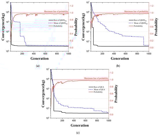
Figure 6.
Convergence graph of 20-bar truss structures: (a) QbHS. (b) QbHS. (c) QE.
Figure 7 is the size of each cross-sectional area derived as a result of weight optimization of a 20-bar truss structure, and the red dot line is the maximum cross-sectional area that an element can have. Even though the cross-sectional area is different, all three algorithms adopted 1, 5, 8, 11, 13, 15, 18, and 20 elements. The QbHS algorithm additionally adopted 4 elements, and we found that all areas of elements were smaller than the maximum cross-sectional area. As a result, a total of eight elements were selected for the QbHS and QE algorithms, and a total of nine elements were selected for the QbHS algorithms.
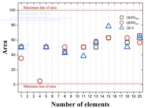
Figure 7.
Result area of 20-bar truss structures.
Table 4 is a table of weight optimization results of a 20-bar truss structure. The best weight was 320.445 kg with the QbHS algorithm. Similarly, Mean weight and Standard Deviation (S.D.) was the best QbHS algorithms at 381.180 kg and 48.792. That is, the results of the QbHS algorithm were the best for weight optimization of the 20-bar truss structure. It can be seen that constraints of , , , and are also satisfied with the results of all algorithms.
Table 4.
Results of 20-bar truss structure.
Figure 8 expresses the weight optimization result of the 20-bar truss structure with an image coordinate system. In this paper, the topology of the truss structure derived as a result of weight optimization is expressed using an image coordinate system. The elements of all structures are made up of two nodes, and each node is given a unique node number. The two node numbers constituting the element may be expressed as coordinates. For example, the first element of Figure 5a consists of the node 1 and node 2. That is, it may be expressed as coordinates of (1, 2) or (2, 1), and the represented figure always has symmetry. Using this method, the initial topology of the 20-bar truss structure can be expressed as Figure 8a by expressing the initial topology of the 20-bar truss structure with an image coordinate system. Figure 5b,c is a figure representing the weight optimization results of three algorithms with an image coordinate system, and the topology of the structure can be easily confirmed only by the figure. The truss structures derived as a result of QbHS and QE algorithms have the same topology. The topology of the truss structure, derived by the QbHS algorithm, has an additional element number 4 consisting of node 4 and node 5. If the topology of the structure is expressed with an image coordinate system, the difference in topology can be easily determined only by the figure, and the topology of the structure can be predicted using a neural network structure algorithm in the future.
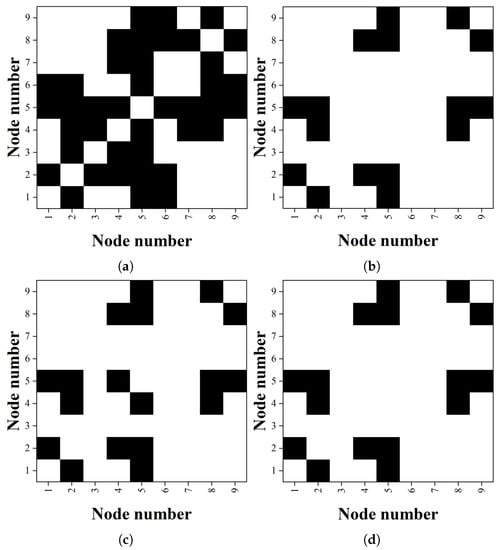
Figure 8.
Image coordinate system of 20-bar truss structure: (a) Basic. (b) QbHS. (c) QbHS. (d) QE.
6.2. 24-Bar Truss Structure
The initial shape of the 24-bar truss structure is shown in Figure 5b, where E and of truss elements are 69,000 MPa and 2740 kg/m3. The range of cross-sectional areas that the element may have is [−40, 40], and the minimum cross-sectional area is 1 cm2. The load acting on a 24-bar truss structure is classified into two conditions. The first condition assumes that 50 kN acts on the x-axis of node 3 and −50 kN on the y-axis of node 6. The second condition assumes that −50 kN acts on the x-axis of node 2 and −50 kN on the y-axis of node 5. Table 5 is a constraint for weight optimization of a 24-bar truss structure. The allowable stress of the element is 172.43 MPa, and the maximum y-axis displacement of node 5 and node 6 is 10 mm. Finally, the first natural frequency of the structure is more than 30 Hz. A total of 100 analyses were conducted, and each analysis was set to 1000 generations.
Table 5.
Constraints of 24-bar truss structures.
Figure 9 is a convergence graph of three algorithms. Solid black, dotted blue and solid red lines indicate the best weight, mean weight, and probability of the Q-bit. The QbHS algorithm derived 125.833 kg, and the QbHS algorithm derived 124.662 kg. The QE algorithm derived 126.565 kg, and the QbHS algorithm derived the smallest weight. All three algorithms show that the Q-bit is almost converged on ‘1’, and using gate, the Q-bit is not fully converged on ‘1’.
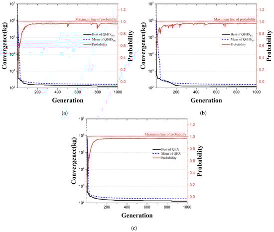
Figure 9.
Convergence graph of 24-bar truss structures: (a) QbHS. (b) QbHS. (c) QE.
Figure 10 is the size of each cross-sectional area derived as a result of weight optimization of the 24-bar truss structure. Elements 7, 8, 13, 15, 16, 22, and 23 were all adopted by three algorithms. The QbHS algorithm additionally adopts the element 4, with all the adopted elements being smaller than the maximum cross-sectional area. As a result, a total of eight elements were selected for the QbHS and QE algorithms, and a total of nine elements were selected for the QbHS algorithms. The QbHS algorithm selected element 10 additionally, and the QbHS algorithm selected element 10 and element 14 additionally. Element 12 was additionally selected for the QE algorithm. In addition, elements 10, 12, 14, 22, and 23 are not necessary for the load burden of the structure, but are necessary by the kinematic ability of the structure.
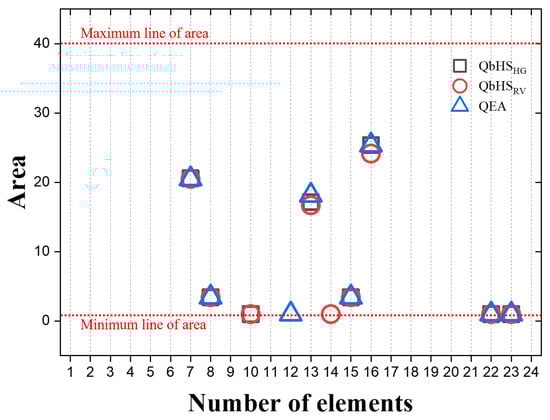
Figure 10.
Result area of 24-bar truss structures.
Table 6 is a table of weight optimization results of a 20-bar truss structure. The best weight was the best with the QbHS algorithm at 124.662 kg, and the mean weight was the best with the QbHS algorithm at 159.394 kg. S.D. had the best QbHS algorithm at 27.702. Conversely, the QE algorithm derived the best weight, mean weight, and S.D. 126.565 kg, 176.130 kg, and 31.798, and derived the worst value. The results of the 24-bar truss structure also show that the constraints of , , , and satisfy all of the results of all algorithms.
Table 6.
Results of 24-bar truss structure.
Figure 11 is a figure representing the weight optimization result of the 24-bar truss structure with an image coordinate system. The initial shape of the 24-bar truss structure is expressed as Figure 5a. The weight optimization results of the 24-bar truss structure all have different topologies depending on the type of algorithm. Based on the topology of the QbHS algorithm with the smallest best weight, the result of the QbHS algorithm is that there is no element 14 composed of node 3 and node 5. As a result of the QE algorithm, there is no element 14 composed of node 3 and node 5, element 10 composed of node 2 and node 8, and there is an additional element 12 composed of nodes 2 and 3.
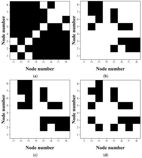
Figure 11.
Image coordinate system of 24-bar truss structure: (a) Basic. (b) QbHS. (c) QbHS. (d) QE.
6.3. 72-Bar Truss Structure
The initial shape of the 72-bar truss structure is shown in Figure 5b, where E and of truss elements are 68,950 MPa and 2767.99 kg/m3. The range of the cross-sectional area that the element may have is [−30 30], and the minimum cross-sectional area is 1 cm2. Additionally, 2270 kg of mass is added to nodes 1–4. The load conditions acting on the 72-bar truss structure are classified into two conditions, as in the previous examples. The first condition assumes that 22.25 kN acts on the x-, y-, and −z-axes of node 1, and the second condition assumes that 22.25 kN acts on the −z-axis of nodes 1–4. Table 7 is a constraint for weight optimization of 72-bar truss structures. The allowable stress of the element is 172.375 MPa, and the maximum displacement of the x- or y-axis at nodes 1–4 is 6.35 mm. Finally, the first natural frequency of the structure is more than 4 Hz, and the third natural frequency is more than 4 Hz. A total of 100 analyses were conducted, and each analysis was set to 1000 generations.
Table 7.
Constraints of 72-bar truss structures.
Figure 12 is a convergence graph of three algorithms. Solid black, dotted blue and solid red lines indicate the best weight, mean weight, and probability of the Q-bit. The QbHS algorithm derived 445.833 kg, and the QbHS algorithm derived 449.190 kg. The QE algorithm derived 446.018 kg, and the QbHS algorithm derived the smallest weight. It can be seen that all three algorithms have almost converged on ‘1’.
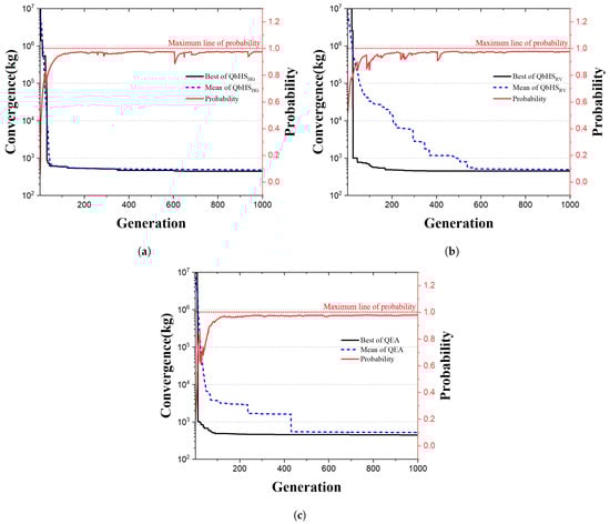
Figure 12.
Convergence graph of 72-bar truss structures: (a) QbHS. (b) QbHS. (c) QE.
Figure 13 is the size of each cross-sectional area derived as a result of weight optimization of the 72-bar truss structure. The groups adopted by all three algorithms are 1, 2, 5, 6, 9, 10, 13, and 14. All algorithms have chosen ten element groups in common, but the total group selected is slightly different. Excluding the common element groups, the QbHS algorithm chose groups 8 and 11 additionally, and the QbHS algorithm chose groups 4 and 15 additionally. The QE algorithm additionally selected groups 8 and 15.
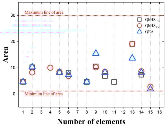
Figure 13.
Result area of 72-bar truss structures.
Table 8 is a table of weight optimization results of a 72-bar truss structure. Best weight, mean weight, and S.D. had the best QbHS algorithm at 445.833 kg, 484.945 kg, and 21.306. All constraints of the 72-bar truss structure were also satisfied. The resulting structure of the QbHS algorithm was the best, with a maximum stress of 48.11 MPa, a maximum buckling stress of 227.11 MPa, and a maximum displacement of 5.323 mm. In addition, the first natural frequency was 4.002 Hz and the third natural frequency was 6.000 Hz.
Table 8.
Results of 72-bar truss structure.
Figure 14 is a figure representing the weight optimization result of the 72-bar truss structure with an image coordinate system. The initial shape of the 72-bar truss structure is expressed in an image coordinate system using a node number as shown in Figure 5a. The weight optimization results of the 72-bar truss structure have different topologies depending on the type of algorithm and can be easily determined by the figure alone.
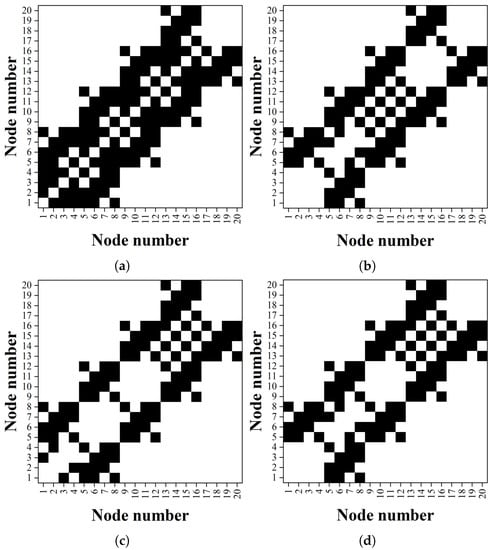
Figure 14.
Image coordinate system of 72-bar truss structure: (a) Basic. (b) QbHS. (c) QbHS. (d) QE.
7. Conclusions
In this paper, we proposed a QbHS algorithm that can solve real variable problems by combining quantum computation and conventional HS algorithms and we used the QbHS algorithm to optimize the size and topology of 20 bar, 24 bar, and 72-bar truss structures.
- The QbHS algorithm maintains the same computational process as the conventional HS algorithm but performs operations using the characteristics of the Q-bit. The of the QbHS algorithm consists of the Q-bit and is classified into QbHS and QbHS algorithms depending on how the Q-bit is initialized. Pitch adjusting is performed using the basic state of the Q-bit, and the Q-bit accumulates information of the previous state. As the number of generations progresses, the Q-bit converges to ‘1’ and converges to one value, and is expressed as binary or real variables through the measurement of the Q-bit. In addition, new termination conditions can be used using the accumulated Q-bit information.
- The weight optimization of the truss structure was performed using the QbHS algorithm proposed in this paper. On the 20-bar truss structure, the QbHS algorithm derived the best results at 320.445 kg, and on the 24-bar truss structure, the QbHS algorithm derived the best results at 124.662 kg. Finally, the 72-bar truss structure derived the best results with a QbHS algorithm of 445.833 kg. That is, the results of the QbHS algorithm proposed in this paper were better than the results of the QE algorithm.
- The topology result of the truss structure that performed weight optimization was expressed with an image coordinate system. The unique node number of the element was expressed as an image coordinate system using the coordinate, and this expression could easily compare the phase of the structure. In addition, if a lot of image coordinate systems are accumulated and used as back data, it is judged that the topology of the structure can be predicted only with pictures using neural network structure algorithms.
The QbHS algorithm proposed in this paper is expected to play a very important role in the expansion of algorithm development and the development of architectural structure design. The QbHS algorithm can be applied to quantum systems if a quantum computer is developed, and a new termination condition can be used with the probability of the Q-bit. However, the number of quantum operations increases due to the measurement of the Q-bit and the inefficient rotation of the Q-bit. Therefore, it is necessary to propose an efficient quantum operation process. Also, for the expansion and globalization of quantum computation-based algorithms, research is needed to apply them to real-world problems such as domes and cable structures as well as large truss structures.
Author Contributions
Conceptualization, S.S., S.L. and J.H.; methodology, S.S. and J.H.; programming, S.S.; validation, D.L. and S.S.; formal analysis, D.L.; investigation, D.L.; data curation, S.S. and D.L.; writing-original draft preparation, D.L. and S.S.; visualization, D.L. and S.S.; supervision, S.S.; project administration, S.L.; funding acquisition, S.L. All authors have read and agreed to the published version of the manuscript.
Funding
This research was supported by Basic Science Research Program through the National Research Foundation of Korea (NRF) funded by the Ministry of Science and ICT (NRF-2019R1A2C2010693).
Institutional Review Board Statement
Not applicable.
Informed Consent Statement
Not applicable.
Data Availability Statement
Not applicable.
Conflicts of Interest
The authors declare no conflict of interest.
References
- Delyová, I.; Frankovskỳ, P.; Bocko, J.; Trebuňa, P.; Živčák, J.; Schürger, B.; Janigová, S. Sizing and topology optimization of trusses using genetic algorithm. Materials 2021, 14, 715. [Google Scholar] [CrossRef]
- Kaveh, A.; Zolghadr, A. Topology optimization of trusses considering static and dynamic constraints using the CSS. Appl. Soft Comput. 2013, 13, 2727–2734. [Google Scholar] [CrossRef]
- Sved, G.; Ginos, Z. Structural optimization under multiple loading. Int. J. Mech. Sci. 1968, 10, 803–805. [Google Scholar] [CrossRef]
- Sheu, C.; Schmit, L., Jr. Minimum weight design of elastic redundant trusses under multiple static loading conditions. AIAA J. 1972, 10, 155–162. [Google Scholar] [CrossRef]
- Ringertz, U.T. On topology optimization of trusses. Eng. Optim. 1985, 9, 209–218. [Google Scholar] [CrossRef]
- Ringertz, U.T. A branch and bound algorithm for topology optimization of truss structures. Eng. Optim. 1986, 10, 111–124. [Google Scholar] [CrossRef]
- Nakamura, T.; Ohsaki, M. A natural generator of optimum topology of plane trusses for specified fundamental frequency. Comput. Methods Appl. Mech. Eng. 1992, 94, 113–129. [Google Scholar] [CrossRef]
- Kirsch, U.; Topping, B. Minimum weight design of structural topologies. J. Struct. Eng. 1992, 118, 1770–1785. [Google Scholar] [CrossRef]
- Sakamoto, J.; Oda, J. A technique of optimal layout design for truss structures using genetic algorithm. In Proceedings of the 34th Structures, Structural Dynamics and Materials Conference, La Jolla, CA, USA, 19–22 April 1993; p. 1582. [Google Scholar]
- Ohsaki, M. Genetic algorithm for topology optimization of trusses. Comput. Struct. 1995, 57, 219–225. [Google Scholar] [CrossRef]
- Su, R.; Wang, X.; Gui, L.; Fan, Z. Multi-objective topology and sizing optimization of truss structures based on adaptive multi-island search strategy. Struct. Multidiscip. Optim. 2011, 43, 275–286. [Google Scholar] [CrossRef]
- Richardson, J.N.; Adriaenssens, S.; Bouillard, P.; Filomeno Coelho, R. Multiobjective topology optimization of truss structures with kinematic stability repair. Struct. Multidiscip. Optim. 2012, 46, 513–532. [Google Scholar] [CrossRef]
- Kuo, H.C.; Chiu, J.T.; Lin, C.H. Intelligent Garbage Can Decision-Making Model Evolution Algorithm for optimization of structural topology of plane trusses. Appl. Soft Comput. 2012, 12, 2719–2727. [Google Scholar] [CrossRef]
- Faramarzi, A.; Afshar, M. Application of cellular automata to size and topology optimization of truss structures. Sci. Iran. 2012, 19, 373–380. [Google Scholar] [CrossRef]
- Kaveh, A.; Laknejadi, K. A hybrid evolutionary graph-based multi-objective algorithm for layout optimization of truss structures. Acta Mech. 2013, 224, 343–364. [Google Scholar] [CrossRef]
- Finotto, V.C.; da Silva, W.R.; Valášek, M.; Štemberk, P. Hybrid fuzzy-genetic system for optimising cabled-truss structures. Adv. Eng. Softw. 2013, 62, 85–96. [Google Scholar] [CrossRef]
- Xu, B.; Jiang, J.; Tong, W.; Wu, K. Topology group concept for truss topology optimization with frequency constraints. J. Sound Vib. 2003, 261, 911–925. [Google Scholar] [CrossRef]
- Savsani, V.J.; Tejani, G.G.; Patel, V.K. Truss topology optimization with static and dynamic constraints using modified subpopulation teaching–learning-based optimization. Eng. Optim. 2016, 48, 1990–2006. [Google Scholar] [CrossRef]
- Savsani, V.J.; Tejani, G.G.; Patel, V.K.; Savsani, P. Modified meta-heuristics using random mutation for truss topology optimization with static and dynamic constraints. J. Comput. Des. Eng. 2017, 4, 106–130. [Google Scholar] [CrossRef]
- Holland John, H. Adaptation in Natural and Artificial Systems; University of Michigan Press: Ann Arbor, MI, USA, 1975. [Google Scholar]
- Kirkpatrick, S.; Gelatt, C.D., Jr.; Vecchi, M.P. Optimization by Simulated Annealing. Science 1983, 220, 671–680. [Google Scholar] [CrossRef] [PubMed]
- Kennedy, J.; Eberhart, R. Particle swarm optimization. In Proceedings of the ICNN’95—International Conference on Neural Networks, IEEE, Perth, WA, Australia, 27 November–1 December 1995; Volume 4, pp. 1942–1948. [Google Scholar]
- Rao, R.V.; Savsani, V.J.; Vakharia, D. Teaching–learning-based optimization: A novel method for constrained mechanical design optimization problems. Comput.-Aided Des. 2011, 43, 303–315. [Google Scholar] [CrossRef]
- Morsch, O. Quantum Bits and Quantum Secrets: How Quantum Physics Is Revolutionizing Codes and Computers; John Wiley & Sons: Hoboken, NJ, USA, 2008. [Google Scholar]
- National Academies of Sciences, Engineering, and Medicine. Quantum Computing: Progress and Prospects; National Academies Press: Washington, DC, USA, 2019. [Google Scholar]
- Han, K.H.; Kim, J.H. Genetic quantum algorithm and its application to combinatorial optimization problem. In Proceedings of the 2000 Congress on Evolutionary Computation, CEC00 (Cat. No. 00TH8512), IEEE, La Jolla, CA, USA, 16–19 July 2000; 2, pp. 1354–1360. [Google Scholar]
- Han, K.H.; Kim, J.H. Quantum-inspired evolutionary algorithm for a class of combinatorial optimization. IEEE Trans. Evol. Comput. 2002, 6, 580–593. [Google Scholar] [CrossRef]
- Ross, O.H.M. A review of quantum-inspired metaheuristics: Going from classical computers to real quantum computers. IEEE Access 2019, 8, 814–838. [Google Scholar] [CrossRef]
- Geem, Z.W. Harmony search in water pump switching problem. In Advances in Natural Computation: First International Conference, ICNC 2005, Changsha, China, 27–29 August 2005, Proceedings, Part III 1; Springer: Berlin/Heidelberg, Germany, 2005; pp. 751–760. [Google Scholar]
- Wang, L.; Zhou, P.; Fang, J.; Niu, Q. A hybrid binary harmony search algorithm inspired by ant system. In Proceedings of the 2011 IEEE 5th International Conference on Cybernetics and Intelligent Systems (CIS), IEEE, Qingdao, China, 17–19 September 2011; pp. 153–158. [Google Scholar]
- Layeb, A. A hybrid quantum inspired harmony search algorithm for 0–1 optimization problems. J. Comput. Appl. Math. 2013, 253, 14–25. [Google Scholar] [CrossRef]
- Alfailakawi, M.G.; Ahmad, I.; Hamdan, S. Harmony-search algorithm for 2D nearest neighbor quantum circuits realization. Expert Syst. Appl. 2016, 61, 16–27. [Google Scholar] [CrossRef]
- Geem, Z.W.; Kim, J.H.; Loganathan, G.V. A new heuristic optimization algorithm: Harmony search. Simulation 2001, 76, 60–68. [Google Scholar] [CrossRef]
- Qin, F.; Zain, A.M.; Zhou, K.Q. Harmony search algorithm and related variants: A systematic review. Swarm Evol. Comput. 2022, 101126. [Google Scholar] [CrossRef]
- Finotto, V.; Lucena, D.; da Silva, W.L.; Valášek, M. Quantum-inspired evolutionary algorithm for topology optimization of modular cabled-trusses. Mech. Adv. Mater. Struct. 2015, 22, 670–680. [Google Scholar] [CrossRef]
- Srikanth, K.; Panwar, L.K.; Panigrahi, B.K.; Herrera-Viedma, E.; Sangaiah, A.K.; Wang, G.G. Meta-heuristic framework: Quantum inspired binary grey wolf optimizer for unit commitment problem. Comput. Electr. Eng. 2018, 70, 243–260. [Google Scholar] [CrossRef]
- McMahon, D. Quantum Computing Explained; John Wiley & Sons: Hoboken, NJ, USA, 2007. [Google Scholar]
- Han, K.H.; Kim, J.H. Quantum-inspired evolutionary algorithms with a new termination criterion, Hϵ gate, and two-phase scheme. IEEE Trans. Evol. Comput. 2004, 8, 156–169. [Google Scholar] [CrossRef]
- Lee, D.W. Development of Quantum-Based Q-HS Algorithm for Weight Optimization of Truss Structures. Ph.D. Thesis, KOREATECH, Cheonan, Republic of Korea, 2022. [Google Scholar]
- Assimi, H.; Jamali, A.; Nariman-Zadeh, N. Multi-objective sizing and topology optimization of truss structures using genetic programming based on a new adaptive mutant operator. Neural Comput. Appl. 2019, 31, 5729–5749. [Google Scholar] [CrossRef]
- Shon, S.D.; Lee, S.J. Structural optimization of planar truss using quantum-inspired evolution algorithm. J. Korea Inst. Struct. Maint. Insp. 2014, 18, 1–9. [Google Scholar]
Disclaimer/Publisher’s Note: The statements, opinions and data contained in all publications are solely those of the individual author(s) and contributor(s) and not of MDPI and/or the editor(s). MDPI and/or the editor(s) disclaim responsibility for any injury to people or property resulting from any ideas, methods, instructions or products referred to in the content. |
© 2023 by the authors. Licensee MDPI, Basel, Switzerland. This article is an open access article distributed under the terms and conditions of the Creative Commons Attribution (CC BY) license (https://creativecommons.org/licenses/by/4.0/).