Abstract
A fundamental notion in building engineering is the equal displacement rule, which posits that the peak inelastic displacement of a system subjected to a ground motion excitation is approximately equal to the displacement of the same system responding elastically. The purpose of this study is to determine if the equal displacement rule can additionally be applied to wind excitations. To achieve this purpose, bilinear single-degree-of-freedom systems were subjected to B-spline wavelet excitations, Fejér–Korovkin wavelet excitations, and wind excitations derived from wind tunnel tests. The results showed the equal displacement rule generally held for excitations with neutral polarity. The frequency content of the excitation had a significant effect on the response because it shifted the location of the displacement-controlled region of the response spectrum. Duration had a mild effect for excitations with neutral polarity. The effect of stiffness and strength degradation due to gravity loads on the response was more pronounced for short-period structures. For regularly shaped buildings subjected to wind forces, the findings suggest that the equal displacement rule applies in the cross-wind direction however not in the along-wind direction.
1. Introduction
The performance-based design of buildings has evolved beyond the consideration of earthquakes to consideration of additional natural hazards, particularly windstorms [1]. This evolution in design is reflected by the many performance-based frameworks that have been proposed for wind engineering [1,2,3,4,5,6,7,8,9,10]. An important aspect of building performance is inelastic behavior. One reason inelastic behavior is important is that rare, large-magnitude windstorms, such as hurricanes, thunderstorms, derechos, and tornadoes cannot always be mitigated economically using design based on elastic forces. Although several studies have studied the inelastic responses of buildings subjected to wind loads [11,12,13,14,15,16], an examination of the underlying behavior has not been attempted to date. In particular, the role of ductility in an inelastic wind response is not well understood.
A fundamental concept in earthquake engineering is that it is the ductility of the lateral force resisting system and not its strength, that is the key to economically design a building to withstand earthquakes. The importance of ductility for seismic design can be demonstrated by idealizing the lateral system as a single-degree-of-freedom (SDOF) system subjected to a base excitation, as shown in Figure 1. The effective lateral force () that is generated by the motion of the building relative to its base is equivalent to the building mass () times the ground acceleration (). As will be shown later in the paper, the dynamic response of the SDOF system depends primarily on the natural period of vibration () of the building, the viscous damping ratio () assumed in the analysis, and the force versus deformation behavior of the lateral system [11,17].
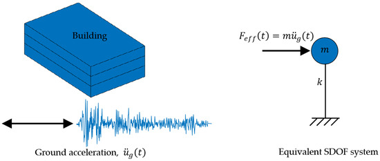
Figure 1.
Idealization of a building subjected to a base excitation as a single-degree-of-freedom (SDOF) system subjected to an effective force excitation.
For ductile lateral systems, the force versus deformation behavior can be approximated using a bilinear relationship. If gravity load effects are not included, the bilinear relationship, shown in Figure 2a, is defined by the lateral system stiffness () and yield strength (). The required ductility is equal to the peak elastic displacement () divided by the yield displacement ( = ). For reference, the figure shows the maximum force that would develop if the system was to remain elastic (). If gravity load effects are included, the bilinear relationship is rotated, as shown in Figure 2b, depending on the ratio of the gravity load to the elastic buckling load of the lateral system, denoted as the stability coefficient (). The effect of the gravity load is a reduced initial stiffness (), a reduced yield strength (), and a negative secondary (post-peak) stiffness ().
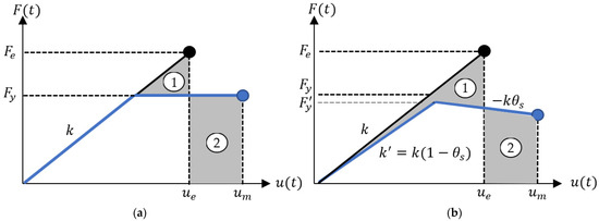
Figure 2.
Bilinear force versus deformation relationship for a lateral system in a building: (a) without gravity load effects; (b) with gravity load effects.
The importance of ductility in earthquake engineering can be illustrated by considering the response of a SDOF system subjected to an acceleration record. In this illustration, the horizontal ground acceleration in the north–south direction that was recorded during the 1940 El Centro earthquake at the Imperial Valley Irrigation District station [17] is used, and the structure is assumed to have 5% viscous damping.
Figure 3a shows the displacement response history for an elastic system, with = 1.0 s. The peak elastic displacement () is equal to 56.9 mm. By comparison, Figure 3b shows the inelastic response of the system if the yield strength is half of that required to keep the system elastic (i.e., = /2 = ). Figure 3c shows the inelastic response if the yield strength is only a quarter of the elastic strength. Interestingly, the example shows that the peak inelastic displacement () is roughly constant, regardless of the yield strength.
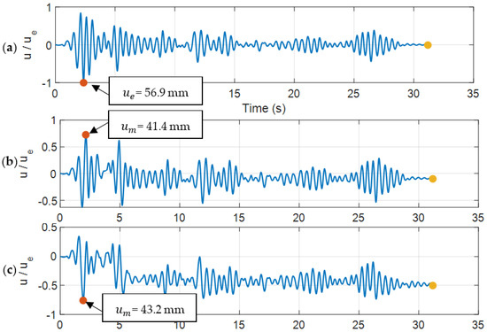
Figure 3.
Displacement response history for 1940 El Centro ground motion and = 1.0 s: (a) elastic SDOF system; (b) inelastic SDOF system with = /2; and (c) inelastic SDOF system with = /4.
Figure 4 shows the ratio of the peak inelastic to peak elastic displacements for a range of periods of vibration and for yield strengths, ranging from 1/2 to 1/8 of the required elastic strength. The figure shows that the ratio of peak inelastic displacement ratio is roughly constant for structures with greater than 0.3 s (sometimes termed as “medium- and long-period” buildings). Since the fundamental period of vibration of most buildings is between 0.1 s and 10 s, the example illustrates that, for most buildings, the displacement of an inelastic lateral system subjected to this specific ground motion is approximately equal to the displacement of the same system responding elastically. Results similar to those shown in Figure 4 have been confirmed for other ground motion records [18] and for other types of force–deformation relationships [19].
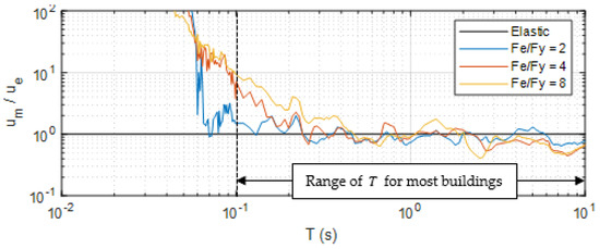
Figure 4.
Inelastic to elastic displacement ratio for SDOF systems subjected to the 1940 El Centro ground motion.
The upshot is that for earthquake ground motions, the displacement is independent of the yield strength of the lateral system. This surprising result was first observed by Veletsos and Newmark [20], and it is commonly known as the “equal displacement rule.” The equal displacement concept has been shown to generally hold true, as long as the strength and stiffness of the system does not degrade, e.g., due to the gravity load effect shown in Figure 2b, fatigue is not an issue, and assuming that the ductility capacity of the lateral system is greater than or equal to the ductility demand.
For “short-period” buildings, where the equal displacement rule does not hold, an alternative assumption that has been proposed in the literature is that the strain energy corresponding to the peak inelastic displacement is equal to the strain energy at the peak elastic response [21]. This is referred to as the “equal energy rule.” The equal energy rule can be checked by comparing the shaded area 1 with the shaded area 2 in Figure 2. If the areas are equal, the equal energy rule holds. However, previous studies have indicated that the equal energy rule is questionable [22,23,24]. As a consequence, most design provisions in the United States and Europe are based on the equal displacement rule [25].
The implication of the equal displacement rule in earthquake engineering is that a building can be designed for a reduced lateral force if the lateral system is capable of deforming proportional to that reduction and if the lateral system can sustain inelastic cycles without a loss of strength or stiffness. As a result, the key objective in performance-based seismic design is to provide ductility. However, it is unclear how ductility should be applied in performance-based wind design.
The purpose of this study is to determine if the equal displacement rule can additionally be applied to wind forces. To achieve this purpose, bilinear SDOF systems were subjected to two types of excitations: wavelet-based excitations and wind excitation derived from wind tunnel test data. This study examines SDOF systems instead of multi-degree-of-freedom (MDOF) systems because the response of SDOF systems is the basis for the equal displacement rule in the literature e.g., [11,17,20]. Although the focus of this study is on wind excitations, the principal conclusions could additionally be applied to other types of excitations.
This paper is organized as follows. First, the methodology is described: the approach used to generate wavelet-based excitations is explained, and the process is used to determine wind-force excitations based on wind tunnel test data. Second, the results are presented: the effect of polarity, frequency content of the excitation, duration, and stiffness and strength degradation due to gravity loads on the wavelet response is discussed, followed by a discussion of the effect of wind directionality and duration on the wind response. Third, the core findings and their implications for performance-based wind design are discussed.
2. Methodology
This study used a nonlinear dynamic response history analysis of bilinear SDOF systems to interrogate the effect of excitation characteristics on the peak inelastic displacement ratio. Figure 5 shows a flow chart of the methodology. The systems were subjected to two types of excitations: wavelet-based excitations and wind force excitations. To the authors’ knowledge, this is the first time that wavelets have been used to examine the equal displacement and equal energy rules. Linear response history analyses were run to determine the elastic response and to generate the displacement, velocity, and acceleration spectra. Nonlinear response history analyses were run to determine the inelastic response. For the response history analyses, the equation of motion was solved iteratively using implicit direct time integration by employing Newmark’s constant average acceleration method [26]. Newton–Raphson iterations were used to achieve convergence for nonlinear systems. The difference at each time step between external energy from the excitation and the internal energy was used to assess the quality of the numerical solution.

Figure 5.
Flow chart of the methodology.
2.1. Wavelet-Based Excitation
The wavelet-based excitations are shown in Figure 6. A wavelet is a waveform of finite duration, with neutral polarity (a mean amplitude equal to zero). Wavelets were utilized in this study because they permit the fundamental characteristics of a waveform, such as frequency content, duration, symmetry, and polarity to be controlled directly. In contrast, waveforms based on recorded data from a ground motion or from a wind tunnel test are stochastic, and therefore, their characteristics cannot be controlled other than through record selection and spectrum matching techniques [27].
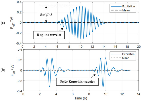
Figure 6.
Wavelet-based excitations: (a) B-spline function; (b) Fejér–Korovkin wavelet.
This study used two types of wavelets: a complex frequency wavelet constructed using a basis-spline function (B-spline wavelet) [28] and a Fejér–Korovkin wavelet constructed using a multiresolution analysis filter [29]. These wavelets were selected because they have complementary features. The B-spline wavelet frequency allows the frequency content of the excitation to be controlled directly, and the Fejér–Korovkin wavelet allows the excitation to be asymmetric with respect to both amplitude and time, while still maintaining neutral polarity. As a result, these wavelets exhibit characteristics (e.g., frequency content, duration, and symmetry) that are related to wind forces.
The B-spline wavelet is shown in Figure 5a. It is defined by the following equation:
where ψ is the complex wavelet of integer order , is the center frequency of the wavelet, is the bandwidth parameter (frequency range), is the imaginary unit, and is time. The parameter is additionally used in the denominator of the sine term. In this study, was 3, and the upper and lower bounds of the waveform duration were 10 s. The real component of the wavelet was used to define the excitation force, . To investigate the effect of a polarity (i.e., a non-symmetric amplitude), the amplitude was offset relative to the mean force () or the positive values of the effective force were multiplied by a scaling factor (), as follows:
In Figure 6, the amplitude () is normalized by the weight based on a unit mass. If , the B-spline wavelet is symmetric about both axes (time and amplitude). The center frequency and bandwidth were adjusted to examine the effect of the frequency content and duration.
The second type, shown in Figure 6b, was a Fejér–Korovkin wavelet constructed using a multiresolution analysis filter [29]. In this study, the wavelet was flipped (reversed) to better reflect the nonstationary aspects of natural (wind and seismic) excitations. In contrast to the B-spline wavelet, the Fejér–Korovkin wavelet is not symmetric in time or amplitude. The frequency content is controlled by scaling (stretching or compressing) the wavelet. The duration is adjusted by repeating the wavelet. In this study, the wavelet was repeated once, as shown in Figure 6b, so that the cumulative duration of the excitation was comparable to the duration of the B-spline wavelet shown in Figure 6a.
A comparison of the elastic response spectra for the wavelet excitations is shown in Figure 7. The elastic response spectrum was generated by solving the equation of motion through an interpolation of the excitation over each time step [17]. This solution method was used because it is exact for linear elastic systems. For each period of vibration, the peak displacement (maximum absolute value) response was saved and used to compute the peak pseudo-velocity and peak pseudo-acceleration. For low levels of damping (e.g., 5%), the pseudo values are approximately the same as the true values.
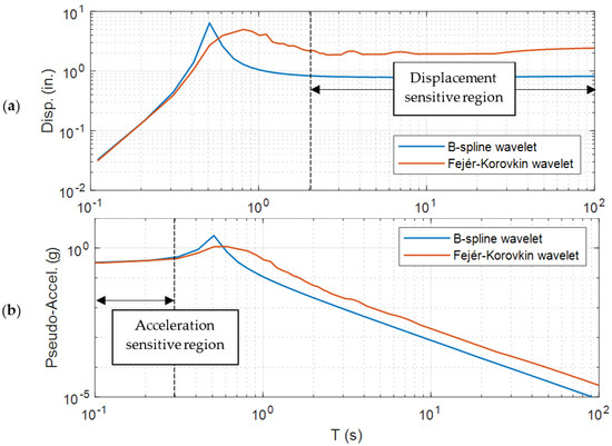
Figure 7.
Elastic response spectra for wavelet excitation: (a) displacement; (b) acceleration.
The smooth shape of the spectrum for the B-spline wavelet reflects the regularity of the waveform. Likewise, the rough spectrum for the Fejér–Korovkin wavelet reflects the irregularity of the waveform. For both types of wavelet excitations, the displacement spectrum (Figure 7a) shows that systems with approximately 2 s are sensitive to displacement, and the pseudo-acceleration spectrum (Figure 6b) shows that systems with approximately 0.3 s are sensitive to acceleration. These period regions are important because the equal displacement rule is known to hold in the displacement-sensitive region, and the equal energy rule is thought to hold in the acceleration-sensitive region [17].
2.2. Wind Force Excitation
The wind force excitation used in this study was derived from wind tunnel test data for a three-story building. A small-scale model of the building was tested in an aerodynamic boundary layer wind tunnel [30]. The recorded data are publicly available at the United States National Institute of Standards and Technology (NIST) website, under the “im1” model archive in the NIST database (https://www.nist.gov/) (accessed on 7 July 2023). The model corresponds to a full-scale building that is 24.4 m wide, 38.1 m long, and 12.2 m tall.
In the wind tunnel tests, the surfaces of the model were instrumented with an array of pressure taps, as shown in Figure 8. The external pressure coefficient () history was recorded at each pressure tap. The external pressure coefficient, , recorded in the wind tunnel tests was referenced to the upper level of the wind tunnel, and it was based on a mean hourly wind speed of 14.3 m/s. Consequently, the values of and corresponding time step () from the wind tunnel database were converted to equivalent full-scale values that are compatible with ASCE 7-22 [31], which references a 10 m height and uses a 3 s gust wind speed. The values were then scaled, so that the full-scale wind speed was 98.4 m/s. This wind speed was intended to be representative of a strength-level wind speed for inelastic wind design. The wind force was computed, based on the tributary area of each pressure tap and building story. Finally, the original wind record was modified so that it linearly ramped up to the full wind intensity and linearly ramped down to zero intensity. The length of the middle (full intensity) segment of the modified record was adjusted to produce 2 durations: a 24 min wind force excitation and a 1 hr wind force excitation. These wind excitations are relevant to real-world wind conditions because they emulate the stationarity of short-duration wind events (e.g., thunderstorms) and long-duration wind events (e.g., synoptic wind or hurricanes).
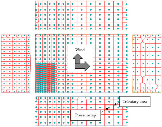
Figure 8.
Wind tunnel model surfaces showing pressure tap layout and tributary areas.
The resulting wind forces on the transverse lateral system () for the 24 min wind event are shown in Figure 9. The amplitude () is normalized by the building weight (5719 kN). The wind parallel to the transverse walls produces “along wind” excitation (Figure 9a), and the wind perpendicular to the transverse walls produces “cross wind” excitation (Figure 9b). For reference, the elastic design force () for the transverse lateral system is shown, based on ASCE 7-22 and typical wind load parameters. The elastic response spectra for the wind-force excitations are shown in Figure 10.
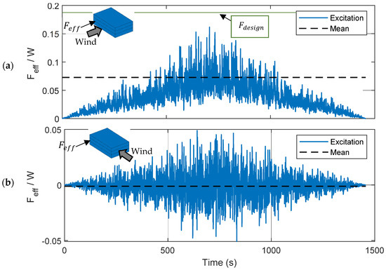
Figure 9.
Wind history for 24 min wind event: (a) along-wind excitation; (b) cross-wind excitation.
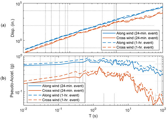
Figure 10.
Elastic response spectra for wind force excitations: (a) displacement; (b) acceleration.
2.3. Nonlinear Response History Analysis
The equation of motion for a SDOF system is given in Equation (3):
where the damping constant ( is equal to . The equation of motion was solved using Newmark’s method. This method is a numerical time-stepping solution, relating acceleration to velocity and acceleration to displacement as follows:
where β and γ are constants that depend on the assumed variation in acceleration. The solution is based on force equilibrium at time i + 1. In this study, the acceleration was assumed to be constant (equal to the average acceleration) over the time step. Thus, β = ¼ and γ = ½.
Newmark’s constant average acceleration method was used because it is relatively efficient compared to explicit integration methods, unconditionally stable for linear analysis, conditionally stable for nonlinear analysis, and generally effective for bilinear and elastoplastic behavior. The bilinear relationship force–deformation relationship followed the initial stiffness, , until yielding and the secondary (post-peak) stiffness () after yielding. Unloading followed the initial stiffness.
Newton–Raphson iterations were used to achieve convergence for nonlinear systems. The difference at each time step between external energy from the excitation and the internal energy was used to assess the quality of the numerical solution. Since the excitations in this study caused an inelastic response, the viscous damping in the equation of motion was set to 5%.
3. Results
The relationship between the peak inelastic displacement ratio, or the peak inelastic energy ratio, the period of vibration, and the yield strength ratio () is shown as a three-dimensional surface (e.g., Figure 11 and Figure 12). The yield strength ratio ranges from 1 to 8 for the wavelet-based excitations. This range covers all the lateral systems currently listed in ASCE 7-22 Table 12.2-1 [31]. For the wind force excitations, the yield strength ratio ranges from 1 to 2. A smaller range was used for the wind force figures, based on the range of yield strength ratios identified in previous studies [11,12]. The period range in the figures covers most buildings, as discussed previously. For reference, the equal displacement () plane or equal energy () plane is superimposed on the surface.
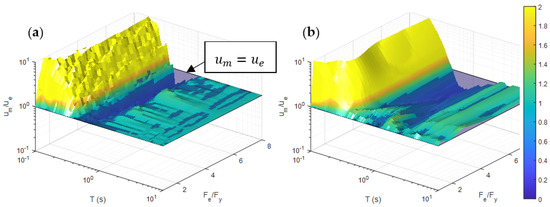
Figure 11.
Peak inelastic displacement ratio: (a) B-spline wavelet; (b) Fejér–Korovkin wavelet.
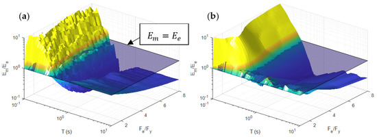
Figure 12.
Peak inelastic energy ratio: (a) B-spline wavelet; (b) Fejér–Korovkin wavelet.
3.1. Wavelet-Based Excitation
The results for the B-spline wavelet (Figure 11a) show that the equal displacement rule holds in the displacement-sensitive region, however not in the acceleration-sensitive region. This finding agrees with the literature e.g., [17]. The results additionally reveal that the peak inelastic displacement is actually smaller than the peak elastic displacement for periods of vibration near the center frequency of the wavelet (the trough region in the surface). These results are essentially independent of the yield strength ratio. The results for the Fejér–Korovkin wavelet (Figure 11b) are basically the same, except that for low yield strength ratios the peak inelastic and peak elastic displacements are similar (there is no trough).
For both types of wavelets, results show that the equal energy rule generally does not hold, even in the acceleration-sensitive region. In the velocity- and displacement-sensitive regions, the peak inelastic energy is much smaller than the peak elastic energy: up to 90% less for high yield strength ratios.
The roughness in the surfaces of the B-spline wavelet reflects the band of high frequency content in the excitation. In contrast, the Fejér–Korovkin wavelet does not contain a similar band of high frequency content. As a result, the surfaces of the Fejér–Korovkin wavelet are smoother.
The effect of polarity on the B-spline wavelet response is shown in Figure 13. The polarity of the excitation has a profound effect on the peak inelastic displacement. A 1% amplitude bias ( = 1.01) significantly narrows the displacement sensitive (flat) region of the spectrum (Figure 13a). As a consequence, the equal displacement rule does not hold for long-period systems (Figure 13b). In the same way, a 1% offset in the mean force shifts the displacement spectrum and narrows the displacement-sensitive region.
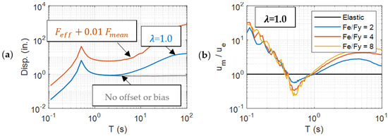
Figure 13.
Effect of polarity on the B-spline wavelet response: (a) displacement spectrum; (b) peak inelastic displacement ratio for 1% amplitude bias.
The effect of frequency content on the B-spline wavelet response is shown in Figure 14. Frequency content has a significant effect, as expected. The frequency content alters the extent of the acceleration and displacement-controlled regions. Frequency content additionally affects the smoothness of the response. High frequency content produces a rough response, and low frequency content produces a smooth response. Gravity loads affect the response of short-period systems more than long-period systems, as shown in Figure 15.
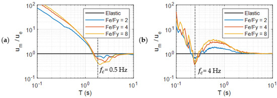
Figure 14.
Peak inelastic displacement ratio for B-spline wavelet: (a) 0.5 Hz; (b) 4 Hz center frequency.
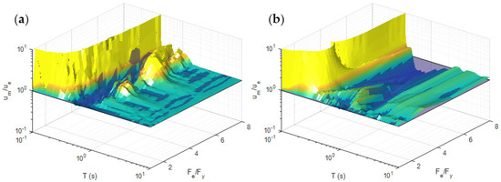
Figure 15.
Peak inelastic displacement ratio for = 2.5%: (a) B-spline; (b) Fejér–Korovkin wavelets.
3.2. Wind Force Excitation
The results for the wind force excitations are shown in Figure 16 and Figure 17. The results indicate that the equal displacement rule does not hold for along-wind forces (Figure 16a); however, the rule holds in a limited sense for cross-wind forces (Figure 16b), with an increased fidelity for long-period systems. The primary factor contributing to the deviation from the equal displacement rule in the along-wind direction is the lack of neutral polarity (the mean wind force is not zero). The results for the peak inelastic energy ratio (Figure 17) follow this pattern, however with less fidelity to the equal energy rule. The ribbed topography of the surfaces reflects the broad band of frequency content inherent in wind excitation. The results indicate that the equal displacement rule might not hold for other orientations of wind because the mean wind force will probably not be zero.
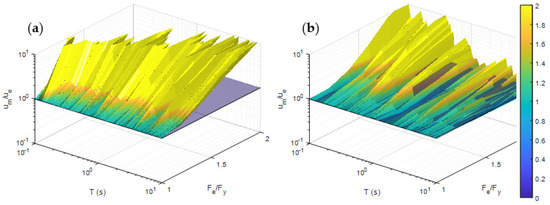
Figure 16.
Peak inelastic displacement ratio: (a) along-wind forces; (b) cross-wind forces.
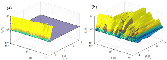
Figure 17.
Peak inelastic energy ratio: (a) along-wind forces; (b) cross-wind forces.
The implication of polarity for wind loading is demonstrated in Figure 18. The results indicate that an excitation with a non-zero mean effective force generates an inelastic response that deviates from the equal displacement rule. For cross-wind loads, the inelastic displacement, even for long-period structures, is five to ten times the elastic displacement, depending on the period and yield strength of the system. These results suggest that ductility does not play as important a role in wind response as it does in seismic response. The results infer the design and safety of buildings in wind-prone regions depends more on strength and stiffness and less on ductility.
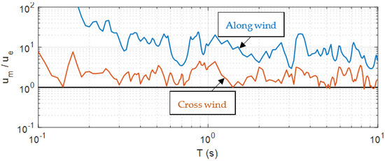
Figure 18.
Peak inelastic displacement ratio for a 1 h wind event and a yield strength ratio of 1.4.
The results demonstrate that the duration of the excitation has an important effect on the response. For example, Figure 19 shows the peak inelastic displacement ratio for systems with a yield strength ratio of 2 that are subjected to short and long duration cross direction wind loads. The longer duration excitation produces larger inelastic displacements. In fact, duration has a similar effect on ground motion excitations. For example, Figure 20 shows the response for a single ground motion record compared to a sequential (repeated) ground motion. To the authors’ knowledge, the effect of the duration of ground motion on the equal displacement rule has not previously been known.
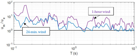
Figure 19.
Peak inelastic displacement ratio for cross-wind forces and a yield strength ratio of 2.
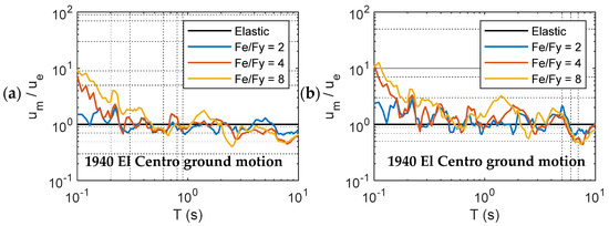
Figure 20.
Peak inelastic displacement ratio for a ground motion: (a) single event; (b) repeated event.
The effect of gravity loads is shown in Figure 21. Gravity load effects are more severe for short-period structures because the second order displacement is large compared to the first order displacement. The equal displacement concept generally does hold in the presence of moderate ( = 2.5%) gravity load effects for cross-wind forces because the excitation is approximately neutral in polarity.
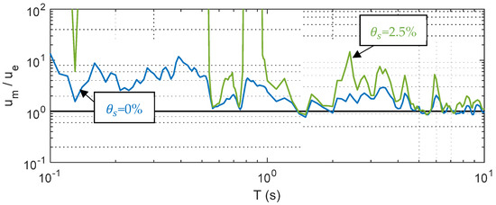
Figure 21.
Effect of gravity loads on the peak inelastic displacement ratio for cross-wind forces and a yield strength ratio of 2.
The physical explanation for this behavior is that as the building displaces, a neutral excitation brings the building back to the undeformed position. At the end of the excitation, the building has zero residual displacement. Thus, gravity load effects do not come into play when the excitation has neutral polarity, and the yield strength ratio is low.
The wind force analysis confirmed the behavior observed in the wavelet analysis. The results showed that the equal displacement concept generally holds for cross-wind excitation, however not for along-wind excitation. The inelastic behavior for cross-wind forces is similar to the inelastic behavior for ground motions, except the equal displacement rule does not hold as well for cross-winds due to the effect of duration. The inelastic behavior for along-wind forces follows the equal displacement rule for a yield strength ratio of 1.2 or less; however, the response is additionally sensitive to duration. The effect of duration is more pronounced for systems with a higher yield strength ratio and a smaller period of vibration. Stiffness and strength degradation due to gravity load effects has a more significant effect on short-period structures compared to long-period structures because second order displacement in stiff structures is relatively large compared to the elastic displacement.
The results demonstrate that the peak inelastic displacement is only equal to the elastic displacement in the displacement-controlled region of the response spectrum (long-period structures). The frequency content of the excitation has a significant effect on the response because it shifts the location of this region. The peak inelastic displacement is only approximately equal to the elastic displacement for long-period structures subjected to excitations with neutral polarity. The results for both wavelet and wind excitations show that the equal energy rule generally does not hold.
Although the focus of this study was on wind excitations, the results from this study illuminate the effect of polarity on the response of seismic ground motions. The results from this study additionally support the findings from earthquake engineering studies [32,33] that show the equal displacement rule does not always hold for spectrum matched ground motions with pulse or non-pulse-like characteristics.
4. Conclusions
Single-degree-of-freedom systems with a bilinear force versus deformation relationship were subjected to wavelet-based excitations and to wind force excitations, based on wind tunnel tests of a low-rise building. Two types of wavelets, B-spline and Fejér–Korovkin wavelets, were used to examine four fundamental characteristics: the polarity (mean amplitude), the frequency content, and the duration of the excitation to be considered. The destabilizing effect of gravity loads was additionally considered. Along-wind and cross-wind force excitations were developed for a three-story building, based on wind tunnel test data. A total of 2 durations were examined: a 24 min wind force excitation and a 1 h wind force excitation. The following are the main findings:
- The polarity of the excitation dominates the inelastic response of the system. The results indicate that a bias of only 1% in the amplitude causes inelastic displacements to grow without bounds, for highly ductile systems for a broad range of a period of vibration. A similar effect is observed for an excitation with only a 1% offset in the mean force;
- The frequency content of the excitation has a significant effect on the inelastic response because it shifts the extent of the displacement-controlled region of the response spectrum;
- The duration of the excitation has a mild effect, compared to polarity and frequency content, for excitations with neutral polarity (a mean amplitude force equal to zero). A repeated excitation has a minor effect on the response, compared to a single excitation;
- The effect of stiffness and strength degradation due to gravity loads on the inelastic response is more pronounced for short-period structures.
These findings suggest that for wind forces, the equal displacement rule could be applied in the cross-wind direction however not in the along-wind or oblique wind directions. If there is even a slight bias to the excitation, the equal displacement concept does not hold. Inelastic displacements increase significantly when the mean-force is not zero. This occurs regardless of gravity loads, whose effect is dwarfed by the effect of polarity. These findings are limited to low-rise buildings with wind events of similar duration and stationarity. Additional research is needed to determine the response of multi-degree-of-freedom systems.
The implication of the findings is that ductility plays less of a role in wind response, compared to seismic response. Furthermore, a reduced wind design force as part of a performance-based design may be applicable in high-rise buildings where cross-wind loads, due to vortex shedding, govern the design of the lateral system; however, in low-rise buildings, where along-wind loads dominate, a reduced design force based on ductility may not be justified in the same way that it is in earthquake engineering.
Author Contributions
Conceptualization, J.J.; methodology, J.J. and J.N.; writing—original draft preparation, J.J.; writing—review and editing, J.N. All authors have read and agreed to the published version of the manuscript.
Funding
This research was funded in part by the American Institute of Steel Construction.
Data Availability Statement
All data products generated in this study are available from the authors upon request.
Conflicts of Interest
The authors declare no conflict of interest. The funders had no role in the design of the study; in the collection, analyses, or interpretation of data; in the writing of the manuscript; or in the decision to publish the results.
References
- American Society of Civil Engineers (ASCE). Prestandard for Performance-Based Wind Design, version 1.1; ASCE: Reston, VA, USA, 2022. [Google Scholar]
- Spence, S.M.J.; Chuang, W.C.; Tabbuso, P.; Bernardini, E.; Kareem, A.; Palizzolo, L.; Pirrotta, A. Performance-based engineering of wind excited structures: A general methodology. In Proceedings of the Structures Congress 2016, Phoenix, AZ, USA, 14–17 February 2016. [Google Scholar]
- Griffis, L.; Patel, V.; Muthukumar, S.; Baldava, S. A framework for performance-based wind engineering. In Advances in Hurricane Engineering; ASCE: Reston, VA, USA, 2012; pp. 1205–1216. [Google Scholar] [CrossRef]
- Kareem, A.; Spence, S.M.J.; Bernardini, E. Performance-Based Design of Wind-Excited Tall and Slender Structures; NatHaz Modeling Laboratory, University of Notre Dame: South Bend, IL, USA, 2013. [Google Scholar]
- Barbato, M.; Petrinib, F.; Unnikrishnana, V.U.; Ciampolib, M. Performance-based hurricane engineering (PBHE) framework. Struct. Saf. 2013, 45, 24–35. [Google Scholar] [CrossRef]
- Hart, G.C.; Jain, A. Performance based wind design of tall concrete buildings in the Los Angeles region utilizing structural reliability and nonlinear time history analysis. In Proceedings of the 12th Americas Conference on Wind Engineering, Seattle, WA, USA, 16–20 June 2013. [Google Scholar]
- van de Lindt, J.W.; Dao, T.N. Performance-based wind engineering for wood-frame buildings. J. Struct. Eng. 2009, 135, 169–177. [Google Scholar] [CrossRef]
- Ciampoli, M.; Petrini, F.; Augusti, G. Performance-based wind engineering: Towards a general procedure. Struct. Saf. 2011, 33, 367–378. [Google Scholar] [CrossRef]
- Abdelwahab, M.; Ghazal, T.; Nadeem, K.; Aboshosha, H.; Elshaer, A. Performance-based wind design for tall buildings: Review and comparative study. J. Build. Eng. 2023, 68, 106103. [Google Scholar] [CrossRef]
- Spence, S.M.J.; Arunachalam, S. Performance-based wind engineering: Background and state of the art. Front. Built Environ. 2022, 8, 830207. [Google Scholar] [CrossRef]
- Judd, J.P.; Charney, F.A. Inelastic behavior and collapse risk for buildings subjected to wind loads. In Proceedings of the Structures Congress, Portland, OR, USA, 17 April 2015; pp. 2483–2496. Available online: https://ascelibrary.org/doi/abs/10.1061/9780784479117.215 (accessed on 7 July 2023).
- Jeong, S.Y.; Alinejad, H.; Kang, T.H.-K. Performance-based wind design of high-rise buildings using generated time-history wind loads. J. Struct. Eng. 2021, 147, 04021134. [Google Scholar] [CrossRef]
- Alinejad, H.; Jeong, S.Y.; Chang, C.; Kang, T.H.-K. Upper limit of aerodynamic forces for inelastic wind design. J. Struct. Eng. 2022, 148, 04021271. [Google Scholar] [CrossRef]
- Athanasiou, A.; Tirca, A.L.; Stathopoulos, T. Nonlinear wind and earthquake loads on tall steel-braced frame buildings. J. Struct. Eng. 2022, 148, 04022098. Available online: https://ascelibrary.org/doi/abs/10.1061/%28ASCE%29ST.1943-541X.0003375 (accessed on 7 July 2023). [CrossRef]
- Ghaffary, A.; Moustafa, M.A. Performance-based assessment and structural response of 20-story SAC building under wind hazards through collapse. J. Struct. Eng. 2021, 147, 04020346. [Google Scholar] [CrossRef]
- Mohammadi, A.; Azizinamini, A.; Griffis, L.; Irwin, P. Performance assessment of an existing 47-story high-rise building under extreme wind loads. J. Struct. Eng. 2019, 145, 04018232. [Google Scholar] [CrossRef]
- Chopra, A.K. Dynamics of Structures: Theory and Applications to Earthquake Engineering, 6th ed.; Pearson: Hoboken, NJ, USA, 2023; p. 232. [Google Scholar]
- Chopra, A.K.; Chintanapakdee, C. Inelastic deformation ratios for design and evaluation of structures: Single-degree-of-freedom bilinear systems. J. Struct. Eng. 2004, 130, 1309–1319. [Google Scholar] [CrossRef]
- Miranda, M.; Ruiz-Garcia, J. Evaluation of approximate methods to estimate maximum inelastic displacement demands. Earthq. Eng. Struct. Dyn. 2002, 31, 539–560. [Google Scholar] [CrossRef]
- Veletsos, A.S.; Newmark, N.M. Effect of inelastic behavior on the response of simple systems to earthquake motions. In Proceedings of the Second World Conference on Earthquake Engineering, Tokyo, Japan, 11–18 July 1960; Volume II. [Google Scholar]
- Newmark, N.M.; Hall, W.J. Earthquake Spectra and Design; EERI monograph series; Earthquake Engineering Research Institute: Oakland, CA, USA, 1982. [Google Scholar]
- Michel, C.; Lestuzzi, P.; Lacave, C. Simplified non-linear seismic displacement demand prediction for low period structures. Bull. Earthq. Eng. 2014, 12, 1563–1581. [Google Scholar] [CrossRef]
- Miranda, E. Reflections on the use of elastic or secant stiffness for seismic evaluation and design of structures. In Proceedings of the 1st European Conference of Earthquake Engineering and Seismology, Geneva, Switzerland, 3–8 September 2006. [Google Scholar]
- Ye, L.; Otani, S. Maximum seismic displacement of inelastic systems based on energy concept. Earthq. Eng. Struct. Dyn. 1999, 28, 1483–1499. [Google Scholar] [CrossRef]
- Pavel, F.; Vacareanu, R. Review of methodologies for displacement checks in modern seismic design codes. Buildings 2023, 13, 940. [Google Scholar] [CrossRef]
- Newmark, N.M. A method of computation for structural dynamics. J. Eng. Mech. Div. 1959, 85, 67–94. [Google Scholar] [CrossRef]
- NEHRP Consultants Joint Venture. Selecting and Scaling Earthquake Ground Motions for Performing Response-History Analyses; NIST GCR 11-917-15; National Institute of Standards and Technology: Gaithersburg, MD, USA, 2011. [Google Scholar]
- Teolis, A. Computational Signal Processing with Wavelets; Birkhäuser: Boston, MA, USA, 1998. [Google Scholar] [CrossRef]
- Nielsen, M. On the construction and frequency localization of finite orthogonal quadrature filters. J. Approx. Theory 2001, 108, 36–52. [Google Scholar] [CrossRef]
- Ho, T.C.E.; Surry, D.; Morrish, D.P. NIST/TTU Cooperative Agreement—Windstorm Mitigation Initiative: Wind Tunnel Experiments on Generic Low Buildings, BLWT-SS20-2003, May, 2003. Available online: https://www.nist.gov/system/files/documents/2017/08/03/blwt-ss20-2003.pdf (accessed on 7 July 2010).
- American Society of Civil Engineers (ASCE). Minimum Design Loads and Associated Criteria for Buildings and Other Structures; ASCE: Reston, VA, USA, 2022. [Google Scholar]
- Demir, A.; Palanci, M.; Kayhan, A.H. Probabilistic assessment for spectrally matched real ground motion records on distinct soil profiles by simulation of SDOF systems. Earthq. Struct. 2021, 21, 395–411. [Google Scholar] [CrossRef]
- Kayhan, A.H.; Demir, A.; Palanci, M. Statistical evaluation of maximum displacement demands of SDOF systems by code-compatible nonlinear time history analysis. Soil Dyn. Earthq. Eng. 2018, 115, 513–530. [Google Scholar] [CrossRef]


Disclaimer/Publisher’s Note: The statements, opinions and data contained in all publications are solely those of the individual author(s) and contributor(s) and not of MDPI and/or the editor(s). MDPI and/or the editor(s) disclaim responsibility for any injury to people or property resulting from any ideas, methods, instructions or products referred to in the content. |
© 2023 by the authors. Licensee MDPI, Basel, Switzerland. This article is an open access article distributed under the terms and conditions of the Creative Commons Attribution (CC BY) license (https://creativecommons.org/licenses/by/4.0/).