Comparative Analysis of the Mechanical Performance of Timber Flat Truss Typologies for Different Strength Classes via Optimization Algorithm

Abstract

This study aimed to compare the mechanical performance of two truss typologies, the modified Fan and Howe trusses, using five different wood species: Cambará-rosa, Cupiúba, Angelim-pedra, Garapa, and Jatobá. The spans considered were 6, 9, 12, and 15 m, and the optimization algorithm used was a swarm intelligence algorithm to minimize the structure weight. The study found that wood is a sustainable and viable option for truss constructions, with different wood species having distinct mechanical properties that must be considered when designing the structure. The Howe truss typology presented lower results for the objective function in comparison with the modified Fan truss. The distribution of normal forces in the truss correlated with the characteristic strength in compression and tensile of the species. The Howe truss typology presented a larger amplitude in relation to the modified Fan truss typology in most of the conditions adopted for the Ultimate Limit State constraints. Constraints associated with deflection in the immediate condition were observed to limit the optimization process. The study used the matrix analysis method to evaluate internal efforts and nodal displacements in the trusses. In summary, this study demonstrates the importance of considering all constraints when dimensioning timber structures and the benefits of using different wood species for sustainable construction.

1. Introduction

Wood is a widely used natural resource in civil construction, both in Brazil and around the world. Its versatility and numerous economic and environmental benefits make it a popular choice for roof structures, bridges, and sheds [1,2,3].

According to Fraga [4], wood competes with conventional materials for civil construction, such as steel and concrete, in terms of mechanical properties and structural strength. In comparison to these materials, wood exhibits a favorable relationship between mechanical strength and density [5,6]. Research conducted by Calil Júnior and Dias [7] indicates that compared to steel, wood presents strength–density ratio values about three times higher in tensile and up to ten times higher in compression when compared to reinforced concrete.

Wood is an incredibly valuable natural resource with remarkable renewability and abundance, particularly when coupled with reforestation policies [8]. Its pivotal role in preserving the environment cannot be overstated. In the field of civil construction, wood stands out as a structural material with significant potential for reducing polluting gas emissions compared to conventional materials such as steel, concrete, and aluminum [9]. Moreover, considering its favorable environmental characteristics, wood emerges as a viable and sustainable option for various structural applications [10,11].

In the northern hemisphere, the use of wood in residential buildings is common, especially in the United States of America (USA). The wood frame system is used in about 90% of the residential buildings in the USA [12,13], with approximately 80 million single-family buildings primarily constructed with wood [14]. Residential construction accounts for approximately 26% of total wood consumption in the United States, highlighting the significant role of wood in the forest products value chain [15].

However, the extensive utilization of wood, often carried out in a predatory manner and without reforestation policies, has led to a decline in global forest areas. According to the Food and Agriculture Organization of the United Nations [16], the total forest area decreased from 4235 million hectares to 4058 million hectares between 1990 and 2020. The Brazilian standard for wooden structures, ABNT NBR 7190 [17], provides the properties of some woods from native forests for structural applications, but certain species have been excluded due to predatory exploitation in the past. Deforestation and unsustainable practices have disrupted the supply–demand relationship, resulting in an increase in the price of wood [18].

An alternative approach to mitigating deforestation is the utilization of wood from planted forests, which consist of fast-growing species such Pinus and Eucalyptus. The cultivation of planted wood has expanded since the 1960s [19], initially to meet the demand of the pulp and paper industry and later expanding into other sectors. It has been estimated that the area of planted forests has increased from 170 million hectares to 292 million hectares between 1990 and 2020 [16].

As mentioned previously, unregulated exploitation of forests without reforestation measures can result in irreversible damage to native forests. However, there are sustainable and responsible methods for extracting wood from native forests, such as incorporating planting programs and cultivating new seedlings. These initiatives aim to replace trees extracted from deforestation sites, which are controlled and authorized by the relevant regulatory agency.

The utilization of wood for structural applications in Brazil presents significant potential due to the rich diversity of species found in the Brazilian flora, as emphasized by Santos et al. [20]. According to Steege et al. [21], the Amazon Basin alone has cataloged 11,194 tree species, 1225 genera, and 140 families between the years of 1707 and 2015. The Amazon Rainforest covers an area of 6,850,476 km². It contains an estimated 16,000 tree species, with the majority located in Brazil (4,102,893 km²). Brazil has already cataloged 7694 species, with an estimated 12,655 species. This vast potential, coupled with a sustainable and responsible exploitation policy, allows for the use of native forest wood for structural applications. However, it is crucial to address prejudices and improper utilization of the material, while also disseminating available technological knowledge to prevent durability issues in structures, as highlighted by Calil Júnior et al. [22].

In Brazil, the ABNT NBR 7190-1 [23] is the standard that outlines the fundamental principles for designing timber structures. This standard takes inspiration from the Euro Code 5 EN 1995-1-1 [24]. When considering timber from planted forests, the strength class is determined through the static bending test. However, it is important to note that ABNT NBR 7190-1 [23], when characterizing wood from native forests, maintains the standard procedure with small-sized and defect-free specimens, in which the compressive strength determines the strength class. There are five strength classes, defined according to the characteristic strength in compression parallel to the fibers ($f_{c0,k}$): D20 (20 < $f_{c0,k}$ < 30 MPa), D30 (30 ≤ $f_{c0,k}$ < 40 MPa), D40 (40 ≤ $f_{c0,k}$ < 50 MPa), D50 (50 ≤ $f_{c0,k}$ < 60 MPa), and D60 ($f_{c0,k}$ > 60 MPa).

Table 1. Strength classes of native forest species defined in tests on defect-free specimens.

Class	${\mathit{f}}_{\mathit{c}0,\mathit{k}}$(MPa)	${\mathit{f}}_{\mathit{v}0,\mathit{k}}$(MPa)	${\mathit{E}}_{\mathit{c}0,\mathit{a}\mathit{v}\mathit{e}}$(MPa)	${\mathit{\rho }}_{12\%}$
D20	20	4	10,000	500
D30	30	5	12,000	625
D40	40	6	14,500	750
D50	50	7	16,500	850
D60	60	8	19,500	1000

presents the characteristic strength in compression parallel to the fibers ($f_{c0,k}$), the characteristic shear strength parallel to the fibers ($f_{v0,k}$), the average value of the modulus of elasticity in compression measured in the direction parallel to the wood fibers ($E_{c0,ave}$), and the density with standard moisture content equal to 12% $\left({\rho }_{12\%}\right)$.

The utilization of wood as a construction material is particularly prevalent in regions with low temperatures, such as the southern part of Brazil [25]. Additionally, wood possesses inherent thermal insulation properties, which contribute to improved thermal performance within buildings [26]. Among the various constructive systems employed, wood frame stands out, having gained significant popularity in the United States for constructing wooden houses, apartments, commercial structures, and industrial buildings. In the realm of building roofs, it is quite common to find wood being used in the form of flat trusses in residential, commercial, industrial, and rural settings. Figure 1 provides examples that depict the utilization of wood in roofing systems.

There are various types of trusses, each with its own characteristics, such as parallel chord, triangular, and trapezoidal trusses. When it comes to rational design, it is essential to compare these different typologies and select the most suitable one for each specific case. Computational intelligence, including optimization processes, can be employed to aid in the design and verification of these truss systems.

The parallel chord truss is a typology in which the top and bottom truss elements, called chords, are parallel to each other, and the diagonals elements follow an increasing pattern. In some instances, the diagonals intersect, forming an “X” shape. This typology is well-suited for longer spans ranging from 20 m and 100 m. Figure 2 depicts examples of commonly used parallel chord trusses.

Trapezoidal trusses feature a slight slope on the upper chord, making them particularly suitable for roof applications. Figure 3 provides examples of trapezoidal trusses commonly used in construction.

On the other hand, triangular trusses are widely employed in roof structures and are well-suited for smaller spans. Figure 4 showcases examples of triangular trusses commonly utilized in building design.

In the design of truss systems for structural projects, manual design can be complex and time-consuming. It often involves a trial-and-error methodology, in which engineers rely on structural analysis software based on matrix analysis or the Finite Element Method (FEM). It is important to note that the results obtained from both methods, such as the stiffness matrix and nodal equivalent forces vector, are generally similar. Engineers establish the dimensions of cross-section geometries through successive attempts, considering project constraints and using responses like displacement, loads, and stresses [27]. This process requires a determination of the ideal conditions of a structural system, which can be challenging, as ideal design conditions may conflict with each other. For example, reducing the mass or volume of a structure can lead to reduced stiffness and larger displacements [28].

Given the complexity of this problem and the many variables involved, manual calculation has been replaced by calculation procedures for structural projects that count on the aid of computational science. This approach is essential to expedite the design of structures, speeding up the process of development, reproduction in scale, and improving the ability to test and refine the design [29].

With the evolution of the sizing procedure from computational methods, structural optimization has become a viable tool, applied to various structural systems, including timber structures such as beams [30,31,32], frames [33], and trusses [29,34,35,36].

Although there are some applications in the optimization of truss structures (or other structural systems) that follow normative requirements for fill performance to compare typologies, few studies have addressed this topic. The comparison between typologies is necessary for rational design, and the aid of computational intelligence, as an optimization process, is needed to perform the sizing and verification of these various typologies.

In the context of optimization processes, there are two types of algorithms: probabilistic and deterministic [37]. The probabilistic algorithm includes aspects of random variations in its formulations and is often used to solve optimization problems with a small number of simulations. However, these algorithms are stochastic in nature, and to achieve convergence with high confidence, many simulations are required [38,39]. On the other hand, deterministic algorithms have the ability to drive or approach the global minimum values of the objective function (OF), although the computational cost is high due to the difficulty of obtaining the derivatives of the OF [40,41]. Deterministic methods always produce the same output for a given set of input data and achieve the global minimum of the function with fewer iterations than probabilistic methods [40,42].

Optimization models are divided into three types: dimensional optimization, shape optimization, and topological optimization [43]. These are presented in Figure 5.

• Dimensional optimization changes the dimensions of the cross sections of the elements that make up the structure. The performance of structures can be improved by means of the optimal cross sections. This can result in increased structural stiffness while decreasing structural weight [44].
• Shape or geometric optimization changes the position of certain nodes, i.e., modifies their coordinates. Shape optimization achieves the optimal shape by modifying predetermined boundaries [44].
• Topological optimization modifies the spatial arrangement of the structure, either by removing material or by changing its structural pattern. Topological optimization is often applied in structural optimization. All settings are based on a model analysis. The result is the optimal material distribution [44].

The probabilistic optimization technique consists of a set of meta-heuristic methods, subdivided into bio-inspired ones, whose mathematical formulation is inspired by nature. In general, meta-heuristics can be classified into single-solution-based methods and population-based methods [45]. Existing population-based algorithms fall into three main categories: evolutionary algorithms (EA), algorithms based on physical concepts, and swarm intelligence.

Swarm intelligence is a meta-heuristic technique of biological-inspired optimization, also known as bio-inspired, that emphasizes the distribution of individual agents to solve complex problems. This technique incorporates the philosophy of the collective behavior of natural species. In comparison to algorithms based on physical concepts, swarm intelligence-based algorithms emphasize the simple collective behavior of individual agents, rather than complex control mechanisms [46]. Different swarm intelligence-based algorithms have been introduced in optimization algorithm applications, such as the Artificial Bee Colony (ABC), the Ant Colony Optimization (ACO) Algorithm, the Bat Algorithm (BA), Particle Swarm Optimization (PSO), and the Firefly Algorithm (FA). FA is widely used in structural optimization processes [29,34,47,48,49].

The optimization methods aim to minimize the mass of the structure or other OF while simultaneously meeting all constraints. This makes it possible to compare the performance between distinct wood species, as well as between distinct typologies with the same basic shape (triangular, rectangular, trapezoidal, etc.) for a given established wood species.

The main objective of this paper is to compare different typologies to minimize wood consumption by examining how different wood species from native forests affect this process. In addition, other objectives of this study include:

• Analyzing the design constraints for each typology.
• Evaluating how stressed the optimized truss is in Ultimate Limit State (ULS) checks.
• Verifying the Serviceability Limit State (SLS) conditions post-optimization.

2. Materials and Methods

For the design procedure, the normative precepts established by ABNT NBR 7190-1 [23] were used for the design of compressed and tensioned parts. The FA was used in the optimization process. The calculation methodology for the objective function (OF), the penalty method, the input parameters of the FA, details of the parametric study performed, wood properties considered for the optimization procedure, and the statistical tool used to compare the studied typologies are described in this chapter.

It is worth noting that the classical formulation of the matrix analysis was considered with the deduction of the stiffness matrix considering the bar element (two nodes and four degrees of freedom for each element). Based on the solution of the equilibrium equation system (equilibrium between external and internal nodal loads), the nodal displacements, stresses, and normal loads in each truss bar were determined.

2.1. Objective Function

The optimization process of the present work aims to minimize the total weight of the truss structural system, a decision based on the study by Kromoser et al. [50], considering nodal displacement constraints, mechanical strength of the bars, minimum dimensions, minimum areas, and geometric criteria due to structural instability. The objective function (OF) is the total weight of the structure, presented in Equation (1), where $A_i$ and $L_{0_i}$ are the cross-sectional area and the length of bar $i$, ${\rho }_i$ is the material density of bar $i$, and $n$ is the number of bars present in the truss.

$$FO \left(A_i, {\rho }_i, L_{0_i}\right)=\sum _i^n{A}_i·{\rho }_i·L_{0_i}$$

(1)

Other factors aside from weight must be considered to optimize truss manufacturing. For example, in industrial manufacturing, it is often more interesting to produce similar elements (same sections) than several sections. This and other aspects can affect the cost of the structure [51,52]. However, the present study only considers weight for optimization, focusing on the final weight of the truss.

2.2. Constraint Treatment

For optimization problems, constraint constraints must be treated. Therefore, the external penalty technique was used [53,54], in which the OF is modified to become a pseudo OF, where $g_j$ represents inequality constraints, and $h_k$ represents constraints on equality. For penalization of the OF, the full form of the external penalty method was applied, as per Equation (2), resulting in the penalized OF ($W$), as presented in Equation (3).

$$P\left(\overrightarrow{x}\right)=\sum _{j=1}^m\max {\left[0,g_j\left(\overrightarrow{x}\right)\right]}^2+\sum _{k=1}^n{\left[h_k\left(\overrightarrow{x}\right)\right]}^2$$

(2)

$$W \left(A_i, {\rho }_i, L_{0_i},\overrightarrow{x} \right)=FO \left(A_i, {\rho }_i, L_{0_i}\right)+R_p·P\left(\overrightarrow{x}\right)$$

(3)

Note that $P\left(\overrightarrow{x}\right)$ is the static external penalty function, as shown in Equation (2). $j$ and $k$ are the j-th inequality constraints and the k-th equality constraints, respectively; $m$ and $n$ are the total number of inequality and equality constraints, respectively; $\overrightarrow{x}$ is the solution vector (random population); $g$ and $h$ are the set of inequality and equality constraints; and $W$ is the penalized OF.

2.3. FA

The Firefly Algorithm (FA) is based on a biologically inspired probabilistic optimization model proposed by Yang (FA) [55]. FA is a population-based method, in which a particle (firefly) moves through a sample space in search of the optimal and feasible solution. In this method, random variable concepts are used to generate the initial population, a random event bounded by the problem [55].

The algorithm was inspired by bioluminescence and the influence of the interaction between fireflies on the mating period. Therefore, the FA optimization method is based on the way in which fireflies can emit light and be perceived by other individuals in the same population.

In the algorithm conception, Yang [55] defined some precepts to aid development, including: all fireflies have a single gender and, having a single gender, are attracted to each other; the attractiveness of each firefly is proportional to its own brightness, but larger distances between individuals decrease such ability.

When the initial population is created, the firefly (design variable) begins to randomly walk, as presented in Equation (4), so that $\overrightarrow{x}$ “moves” according to a design variable update function ($\overrightarrow{\omega }$), in which $\overrightarrow{x}$ is the vector of design variables, $\overrightarrow{\omega }$ is the vector of the update function of $\overrightarrow{x}$, and $t$ is the number of iterations.

$${\overrightarrow{x}}^{t+1}={\overrightarrow{x}}^t+{\overrightarrow{\omega }}^t$$

(4)

Based on this new direction, new positions and possible solutions for the optimal design point are originated [56]. Thus, the fireflies move at each step of the iterative process described in Equation (5).

$${\overrightarrow{\omega }}^t=\beta ·\left({\overrightarrow{x}}_j^t-{\overrightarrow{x}}_i^t\right)+\alpha ·\left(\overrightarrow{\eta }-0.5·\overrightarrow{\epsilon }\right)$$

(5)

where $\beta$ is an attraction term between fireflies $i$ and $j$; ${\overrightarrow{x}}_i$ refers to firefly $i$; ${\overrightarrow{x}}_j$ refers to firefly $j$; $\overrightarrow{\eta }$ is the vector of random numbers between 0 and 1; $\alpha$ is the randomness factor (Equation (6)); and $\overrightarrow{\epsilon }$ is a unit vector.

In order to guarantee randomness in the optimization process, a randomness factor ($\alpha$) is applied, obtained by means of Equation (6), which follows an exponential decay behavior as the number of iterations $t$. The factor $\theta$ is constant (0.98), and ${\alpha }_{min}$ and ${\alpha }_{max}$ are the upper and lower bounds of the randomness factor ($\alpha$).

$$\alpha ={\alpha }_{min}+\left({\alpha }_{max}-{\alpha }_{min} \right)·{\theta }^t$$

(6)

$\beta$ is the attractiveness among fireflies in the swarm, presented in Equation (7), in which ${\beta }_0$ is the attractiveness for a distance $r=0$; $r_{ij}$ is a Euclidean distance between fireflies $i$ and $j$ (Equation (8)); and $\gamma$ is the light absorption parameter (Equation (9)).

$$\beta ={\beta }_0·e^{\gamma ·r_{ij}^2}\cong \frac{{\beta }_0}{\left(1+\gamma ·r_{ij}^2\right)}$$

(7)

$$r_{ij}=\left|{\overrightarrow{x}}_i^t-{\overrightarrow{x}}_j^t\right|=\sqrt{\sum _{k=1}^d{\left({\overrightarrow{x}}_{i,k}-{\overrightarrow{x}}_{i,k}\right)}^2}$$

(8)

$$\gamma =\frac{1}{\left(x_{max}-x_{min}\right)}$$

(9)

From Equations (7) and (8), $k$ is the k-th component of the vector of design variables $\overrightarrow{x}$, d is the number of design variables, $x_{max}$ is the upper bound of the design variables, and $x_{min}$ is the lower bound of the design variables.

FA or any other probabilistic optimization method requires attention in defining the parameters of the algorithm (attractiveness: $\beta$ and $\gamma$; randomness: $\alpha$).

The parameter $\gamma$ is the variation in attractiveness by light absorption $\left\{\gamma \in \left[0,\infty \right)\right\}$, essential for determining the speed of convergence and the behavior of the algorithm. Most range from 0.1 to 10 [55].

The representation of the process flow for optimization via the FA algorithm is presented in Figure 6.

Table 2. FA input parameters.

Parameter	Meaning	Adopted Value
${\beta }_0$	Firefly attractiveness	0.90
$N_{ite}$	Number of iterations	600
$N_{pop}$	Population	120
${\alpha }_{min}$	Minimum randomness factor	0.20
${\alpha }_{max}$	Maximum randomness factor	1.00
$R_p$	Penalty factor	105

presents the parameters used in the present study, based on the sensitivity study of Pereira et al. [49].

2.4. Parameters and Considerations for the Optimization Process

The trusses to be optimized are represented in Figure 7. For the present paper, two types of triangular trusses were considered (modified Fan and Howe, represented in Figure 7a,b, respectively) due to their wide use in the design of sheds. However, it should be noted that this method can be applied to any type of truss. The trusses were divided into four spans with a total length of 6, 9, 12, and 15 m to perform a parametric study. For each of the trusses, the optimization was performed 30 times to obtain a spread of the results. Nodal distances obeying the relation $b=L/6$ and $h=L/24$ were used for all typologies, and design variables (position of the bars) considered ${\overrightarrow{x}}_1$, ${\overrightarrow{x}}_2$, ${\overrightarrow{x}}_3$, ${\overrightarrow{x}}_4$, and ${\overrightarrow{x}}_5$ (Figure 7c, where each color represents the group of bars of the variable number considered, positioned in Figure 7a,b). The generic design variable vector ${\overrightarrow{x}}_i$ is described in

Table 3. Standard nominal cross-section values used as variables.

Dimension	Standard Nominal Values (mm)
Thickness ($b_i$)	16, 19, 22, 25, 32, 38, 50, 63, 75, 100, 125, 150, 175, 200, 250 e 300
Height ($h_i$)	75, 100, 115, 125, 150, 160, 175, 200, 225, 250, 275 e 300

, where $b_i$ is the cross-section thickness of variable $i$, and $h_i$ is the cross-section height of variable $i$. For each bar type, a design variable was used: ${\overrightarrow{x}}_1$ for the bottom chord, ${\overrightarrow{x}}_2$ for the top chord, ${\overrightarrow{x}}_3$ for the diagonals, ${\overrightarrow{x}}_4$ for the secondary uprights, and ${\overrightarrow{x}}_5$ for the main upright.

$${\overrightarrow{x}}_i=\left(b_i;h_i\right)$$

(10)

For optimization problems, a set of distinct variables can be considered, in which each variable has an ordered set of values [57]. Therefore, we considered values for nominal dimensions for lumber according to ABNT NBR ISO 3179 [58]. Based on the standard nominal values, the discrete design variables can assume standard nominal values of the cross-section thickness of a generic bar $i$ ($b_i$) and cross-section height of a generic bar $i$ ($h_i$), assuming the values presented in Table 3.

For each of the adopted spans, dimensions for the shed were established. A graphical representation of the shed dimensions is presented in Figure 8, along with the values of the truss and shed dimensions in

Table 4. Description of the nodal distances of the truss and dimensions of the sheds.

Variable/Shed	Type 1	Type 2	Type 3	Type 4
$L$ (m)	6	9	12	15
$h$ (m)	0.25	0.375	0.5	0.625
$b$ (m)	1	1.5	2	2.5
$H$ (m)	0.75	1.125	1.5	1.875
$H_0$ (m)	5
Inclination (%)	25
$A$ (m)	20	25	30	35
$B$ (m)	6	9	12	15
Distance between trusses (m)	5

.

For the optimization process, 5 wood species were characterized, whose properties were characterized according to ABNT NBR 7190-3 [59]. The specifications admitted for sizing are presented in

Table 5. Specifications for the lumber used in the sizing process.

Type of wood	Sawn
Loading class	Long duration
Moisture class	II
Equilibrium moisture (%)	12
Wood category	1st Category

.

2.5. Design Constraints

As noted before, optimization problems count on a constraint treatment method. For the present work, the external penalty method was used, counting with four inequality constraints ($g_j$) and one equality constraint ($h_k$), for the problem proposed in the present work.

The first inequality constraint ($g_j$) is the geometric verification related to the thickness ($b_i$) of the bars of the truss, where the ABNT NBR 7190-1 standard [23] establishes a minimum thickness ($b_{min}$) of 5 cm. The constraint for the minimum dimension is presented in Equation (11), where $i$ is a generic bar ($i=1, 2, 3, \dots , n_{bars}$), and $n_{barras}$ is the number of bars.

$$g_j\left(\overrightarrow{x}\right)=\frac{b_{min} }{b_i}-1\le 0\hspace{1em}\hspace{1em}\hspace{1em}\hspace{1em}j=87 a 107$$

(11)

In Equation (11), $j$ is the number of the constraint for the geometric minimum dimension check, which was assigned the numbers 87 to 107.

Subsequently, the second inequality constraint ($g_j$) is the geometric verification of the area ($A_i$) of the truss bars, where the ABNT NBR 7190-1 standard [23] establishes a minimum area ($A_{min}$) of 50 cm². The constraint for minimum area is described in Equation (12).

$$g_j\left(\overrightarrow{x}\right)=\frac{A_{min} }{A_i}-1\le 0\hspace{1em}\hspace{1em}\hspace{1em}\hspace{1em}j=108 a 128$$

(12)

From Equation (12), $j$ is the constraint number for the geometric minimum area check, which was assigned the numbers 108 to 128.

Equation (13) presents the inequality constraint ($g_j$), which checks the geometric condition of bar slenderness (${\lambda }_i$), where ${\lambda }_{lim}$ is the limit slenderness index, with 140 and 173 being the values established for compressed and tensioned bars, respectively.

$$g_j\left(\overrightarrow{x}\right)=\frac{{\lambda }_i}{{\lambda }_{lim }}-1\le 0\hspace{1em}\hspace{1em}\hspace{1em}\hspace{1em}j=1 a 21$$

(13)

From Equation (13), $j$ is the constraint number for the geometric verification of maximum slenderness, which has been assigned the numbers 1 to 21.

Equation (14) is the inequality constraint ($g_j$) that is considered from the design in the ULS for normal stress action (${\sigma }_i$) in the tensile or compression bar, where ${\sigma }_{lim}$ is the limit for normal stress.

$$g_j\left(\overrightarrow{x}\right)=\frac{{\sigma }_i}{{\sigma }_{lim }}-1\le 0\hspace{1em}\hspace{1em}\hspace{1em}\hspace{1em}j=22 a 42, 43 a 63, 64 a 84$$

(14)

In Equation (14), $j$ is the constraint number for the normal stress verification on the bars, which was assigned the numbers 22 to 42, 43 to 63, and 64 to 84. This is about the ULS verification when considering combinations 1, 2, and 3, respectively.

The inequality constraint ($g_j$) of the verification of the maximum nodal deflection (${\delta }_{max}$) for the SLS is presented in Equation (15), where ${\delta }_{lim}$ is the limit displacement of the truss.

$$g_j\left(\overrightarrow{x}\right)=\frac{{\delta }_{max} }{{\delta }_{lim}}-1\le 0\hspace{1em}\hspace{1em}\hspace{1em}\hspace{1em}j=85 e 86$$

(15)

In Equation (15), $j$ is the number of the constraint for the verification of the normal stress in the bars, which were assigned the numbers 85 and 86. This is the verification of the SLS when considering combinations 4 and 5, respectively.

2.6. Actions and Loadingss

The definition of the actions acting on the trusses follows the requirements of the standards ABNT NBR 6120 [60], ABNT NBR 6123 [61], and ABNT NBR 8681 [62]. To facilitate understanding, they will be subdivided into two topics: permanent and variable actions.

2.6.1. Dead Loads

The load of a permanent nature acting on the trusses comes from the self-weight of the timber elements and the roof materials.

The estimation of the load originating from the self-weight can be achieved by means of an empirical formula or by adopting profiles for the different positions of the joist. For the present study, the self-weight calculation process was obtained through an iterative process, where the truss self-weight ($PP$) was calculated for each group of bars, where the value is updated at each iteration.

In addition, the self-weight due to the truss elements considered the loading of a thermoacoustic tile ($G$) composed of trapezoidal model metallic tiles in the upper part, filled with insulating material, polyurethane ($PU$) in the central part, and lining model metallic tile in the lower part, considering a load $G$ of 350 N/m² according to the manufacturer’s catalog [63].

To obtain the calculation efforts and displacement, where the permanent actions were considered separately, the weighting coefficients of ABNT NBR 8681 were used [64]:

• Unfavorable effect: ${\gamma }_g=1.4$ e ${\gamma }_g=1.3$ (recommendation for cases of direct permanent actions considered separately, for wood structural elements according to item 6.1 of ABNT NBR 7190-1 [23]);
• Favorable effect: ${\gamma }_g=1.0$.

2.6.2. Variable Loads

ABNT NBR 7190-1 [23] establishes that for common roofs with an inclination of less than or equal to 3%, which are not subject to atypical loads, and in the absence of a specification otherwise, a vertical overload ($Q$) characteristic minimum of 250 N/m² of floor area should be provided in a horizontal projection.

Additionally, the wind loads on the structure were obtained through the guidelines established by ABNT NBR 6123 [61] for rectangular sheds with symmetrical gable roofs, as shown in Figure 8, with the dimensions established in Table 4. The wind loads considered in the structure are presented in Figure 9.

To calculate the design efforts and displacements, as well as the permanent actions, the variable actions were considered separately, considering the following combination factors (${\psi }_0$) and reduction factors (${\psi }_1$ and ${\psi }_2$) for variable loading according to ABNT NBR 8681 [62]:

• Overload on commercial shed roof: ${\gamma }_q=1.5$; ${\psi }_0=0.7$; ${\psi }_1=0.6$; ${\psi }_2=0.4$;
• Wind action: ${\gamma }_q=1.4$; ${\psi }_0=0.6$; ${\psi }_1=0.3$; ${\psi }_2=0$.

2.6.3. Combinations Considered

For dead loads, the truss self-weight load ($PP$) and the load due to the thermoacoustic tile ($G$) of 350 N/m² were considered, and for variable actions, the overload ($Q$) of 250 N/m² and wind overpressure or suction load ($w_{ove}$ or $w_{suc}$) were considered, as shown in Figure 9.

From the influence area, a distance between trusses of 5 m was considered, and the distributed loads will be transformed into nodal loads. Once these are calculated via matrix analysis, the normal stresses in the bars and the nodal displacements enable the combination of stresses and displacements. A matrix analysis algorithm is used for structural analysis.

The combinations used for the design and evaluation of the OF are described in

Table 6. Combinations considered in the design.

Limit State		Dead Load	Variable Load
ULS	Combination 1	$1.4·G+1.3·PP$	$1.5·Q+1.4·w_{ove}·0.6$
	Combination 2	$1.4·G+1.3·PP$	$1.4·w_{ove}+1.5·Q·0.5$
	Combination 3	$1.0·G+1.0·PP$	$1.4·{0.75}^{ \mathrm{a}}·w_{suc}$
SLS	Combination 4 b	$\delta G_{inst}+\delta P{P}_{inst}$	$\delta Q_{inst}+0.3·\delta w_{ove.inst}$
		$\delta G_{inst}+\delta P{P}_{inst}$	$\delta w_{ove.inst}+0.4·\delta Q_{inst}$
	Combination 5 c	$\delta G_{fin}+\delta P{P}_{fin}$	$\delta Q_{fin}$

^a—To ensure the most unfavorable condition of the structure, consideration of actions that have a very reduced acting time (wind or the portion of the mobile loads due to impact) may be multiplied by 0.75. ^b—Instantaneous deflection condition. ^c—Final deflection condition considering the effect of creep.

, with their respective increase coefficients ($\gamma$), combination factor (${\psi }_0$) and reduction factor for variable actions (${\psi }_1$).

2.7. Determination of the Physical and Mechanical Properties of Wood

To obtain the physical and mechanical properties applied to the design, the procedures and methodology for the testing and calculation of the characterization of native forest wood were used according to ABNT NBR 7190-3 [59], considering the premise of lots considered homogeneous according to ABNT NBR 7190-1 [23].

The mechanical properties present distinct values, varying according to the type of loading (bending, compression, tensile, and shear), as well as the direction of load application (longitudinal, tangential, and radial) due to their anisotropic composition [65]. Therefore, the variation between trees of the same species and the form of processing should be made from a certain sample, to stratify it statistically.

In this sense, ABNT NBR 7190-3 [59] establishes the minimum numbers of specimens for species’ characterization. Thus, for a minimal and simplified characterization of poorly known species, a minimum number of 12 and 6 specimens is recommended. These specimens were extracted from homogeneous batches (with a volume greater than 12 m³) of sawn wood. In addition, the specimens should be taken from regions at least 5 times larger than the smallest dimension of the cross section, but not less than 30 cm away from the ends of the pieces.

All tests were performed at the Laboratório de Madeiras e Estruturas de Madeiras (LaMEM) of the Engineering Department (SET) of the University of São Paulo (USP), located in São Carlos, SP, where for each test, 12 specimens were prepared and tested as described in the items below. A total of 360 specimens were tested. The identification (ID) and the popular and scientific names of the five evaluated species are presented in

Table 7. Identification, popular name, and scientific name of the evaluated species.

ID	Popular Name	Scientific Name
01	Cambará-rosa	Erisma sp.
02	Cupiúba	Goupia glabra
03	Angelim-pedra	Hymenolobium petraeum
04	Garapa	Apuleia leiocarpa
05	Jatobá	Hymenaea sp.

. It should be noted that the species were purchased from a lumber company located in the region of São Carlos. These species were chosen based on their respective densities, aiming at distinct resistance classes.

3. Results and Discussion

In this section, the results of the characterization of the five species studied are presented. The results of the optimization process are presented for the Howe truss model. Furthermore, throughout the text, discussions involving the characterization of the wood species and the optimization process will be presented.

3.1. Apparent Density

Table 8. Statistics with sample average values of ${\mathit{\rho }}_{\mathbf{12}\%}$ (kg·m⁻³).

ID	Species	$\overline{\mathit{x}}$	$\mathit{S}\mathit{D}$	$\mathit{C}\mathit{V}$(%)	$\mathit{m}\mathit{i}\mathit{n}$	$\mathit{m}\mathit{a}\mathit{x}$	$\mathit{C}\mathit{I}$
01	Cambará-rosa	682.88	41.56	6.09	620.09	740.14	(659.36; 706.39)
02	Cupiúba	846.42	45.73	5.40	778.40	896.13	(820.55; 872.3)
03	Angelim-pedra	695.77	33.12	4.76	644.57	741.89	(677.03; 714.51)
04	Garapa	896.24	41.29	4.61	828.56	953.91	(872.88; 919.61)
05	Jatobá	1054.23	56.79	5.39	998.02	1148.61	(1022.1; 1086.36)

presents the average value ($\overline{x}$) of the wood bulk density (${\rho }_{12\%}$) in kg·m⁻³ of the evaluated species, the standard deviation ($SD$), the coefficient of variation ($CV$ %), the minimum ($min$) and maximum ($max$) value, and the confidence interval ($CI$) of the average value at a 5% significance level.

To validate the results obtained, it is possible to verify normative values and compare them with results obtained in other studies by means of the mean values and the confidence interval (CI). In this context, for the bulk density of wood (${\rho }_{12\%}$), for dicotyledonous species from native forests, when compared with the values presented by ABNT NBR 7190 [66], values close to those obtained in this study were observed in their confidence intervals.

In the study developed by Lahr et al. [67], the complete characterization of the species Cambará-rosa (Erisma sp.) was performed, obtaining an apparent density (${\rho }_{12\%}$) of 680 kg·m⁻³. Similarly, Silva et al. characterized the species Cupiúba (Goupia glabra), obtaining a density of 840 kg·m⁻³. For the species Angelim-pedra (Hymenolobium petraeum) and Jatobá (Hymenaea sp.), the densities obtained by Teixeira et al. [68] and Lahr et al. [69] were 640 kg·m⁻³ and 1050 kg·m⁻³, respectively. These are values that are close to the results obtained in this study, within the confidence intervals.

3.2. Compression Parallel to the Fibers

Table 9. Statistics of the results obtained for the compressive strength parallel to the fibers $f_{c0}$ (MPa).

ID	Species	$\overline{\mathit{x}}$	$\mathit{S}\mathit{D}$	$\mathit{C}\mathit{V}$(%)	$\mathit{m}\mathit{i}\mathit{n}$	$\mathit{m}\mathit{a}\mathit{x}$	$\mathit{C}\mathit{I}$
01	Cambará-rosa	33.73	5.31	15.74	26.89	42.77	(30.73; 36.73)
02	Cupiúba	55.12	13.25	24.04	38.59	74.17	(47.63; 62.62)
03	Angelim-pedra	65.26	17.1	26.2	38.3	84.6	(55.58; 74.94)
04	Garapa	71.93	7.32	10.18	62.29	86.97	(67.79; 76.07)
05	Jatobá	100.09	9.88	9.87	79.40	105.78	(94.5; 105.68)

shows the average value ($\overline{x}$) of the fiber parallel compressive strength ($f_{c0}$) in MPa of the evaluated species, the standard deviation ($SD$), the coefficient of variation ($CV$ %), the minimum (min) and maximum (max) value, and the confidence interval ($CI$) of the average value at a 5% significance level.

Similarly,

Table 10. Statistics of the results obtained for the modulus of elasticity in compression measured in the direction parallel to the fibers ${\mathit{E}}_{\mathit{c}\mathbf{0}}$ (MPa).

ID	Species	$\overline{\mathit{x}}$	$\mathit{S}\mathit{D}$	$\mathit{C}\mathit{V}$(%)	$\mathit{m}\mathit{i}\mathit{n}$	$\mathit{m}\mathit{a}\mathit{x}$	$\mathit{C}\mathit{I}$
01	Cambará-rosa	13,000.88	2672.5	20.56	9719.72	16,956.5	(11,488.77; 14,512.99)
02	Cupiúba	13,891.98	2674.63	19.25	8847.38	18,974.4	(12,378.67; 15,405.29)
03	Angelim-pedra	11,648.41	2254.44	19.35	8274.85	17,597.9	(10,372.84; 12,923.98)
04	Garapa	17,498.15	2950.39	16.86	12,519.9	21,068.1	(15,828.81; 19,167.49)
05	Jatobá	20,466.62	1765.82	8.63	17,106.4	23,097.2	(19,467.51; 21,465.72)

shows the average value ($\overline{x}$) of the modulus of elasticity in compression measured parallel to the fibers ($E_{c0}$) in MPa of the evaluated species, the standard deviation ($SD$), the coefficient of variation ($CV$ %), the minimum ($max$) and maximum ($min$) value, and the confidence interval ($CI$) of the average value at a 5% significance level.

In the sequence, the characteristic strength values for compression parallel to the fibers ($f_{c0,k}$) were obtained through the sample values ($f_{c0,1}, f_{c0,2}, \dots , f_{c0,n}$) for $n=12$ specimens. The average compressive strength parallel to the fibers ($f_{c0,m}$) is essential for the evaluation of the strength class ($SC$), with the class being D20 (20 < $f_{c0,k}$ < 30 MPa), D30 (30 ≤ $f_{c0,k}$ < 40 MPa), D40 (40 ≤ $f_{c0,k}$ < 50 MPa), D50 (50 ≤ $f_{c0,k}$ < 60 MPa), and D60 ($f_{c0,k}$ > 60 MPa), as presented in

Table 11. Strength classes (SC) and characteristic strength for fiber parallel compression (${\mathit{f}}_{\mathit{c}\mathbf{0},\mathit{k}}$) (MPa).

ID	Species	${\mathit{f}}_{\mathit{c}0,1}$	${\mathit{f}}_{\mathit{c}0,\mathit{m}}$	${\mathit{f}}_{\mathit{c}0,\mathit{k}}$	$\mathit{S}\mathit{C}$
01	Cambará-rosa	26.89	33.73	26.95	D20
02	Cupiúba	38.59	55.12	38.59	D30
03	Angelim-pedra	38.30	65.26	45.68	D40
04	Garapa	62.29	71.93	66.50	D60
05	Jatobá	79.40	100.09	88.43	D60

.

To compare the results obtained in this study, it is possible to verify normative values and compare them with the results obtained in other studies through the mean values and the confidence interval (CI). In this sense, when comparing the results with the average values presented by ABNT NBR 7190 [66] for dicotyledonous species from native forests, it was found that the values of strength and the modulus of elasticity were close to the values obtained in the present study in their confidence intervals.

In the experimental program developed by Lahr et al. [67], a complete characterization of the species Cambará-rosa (Erisma sp.) was performed, in which an average strength in fiber parallel compression ($f_{c0,m}$) of 34 MPa and an average modulus of elasticity in fiber parallel compression of 12,764 MPa were observed. Similarly, Silva et al. [70] characterized the Cupiúba species (Goupia glabra) and obtained an average fiber parallel compressive strength ($f_{c0,m}$) of 57.42 MPa and an average modulus of elasticity of 12,970 MPa. For the species Angelim-pedra (Hymenolobium petraeum) and Jatobá (Hymenaea sp.), the values of the mean parallel compressive strength ($f_{c0,m}$) obtained by Teixeira et al. [68] and Lahr et al. [69] were 55.45 and 94.38 MPa, respectively, and values of 10,850 MPa and 21,759 MPa were obtained for the mean modulus of elasticity in parallel compression to the fibers ($E_{c0,m}$), respectively. These values are close to the results obtained in the present study, within the confidence intervals.

3.3. Tensile Strength Parallel to the Fibers

The mean values ($\overline{x}$) of fiber parallel tensile strength ($f_{t0}$) in MPa of the evaluated species, the standard deviation ($SD$), the coefficient of variation ($CV$ %), the maximum ($max$) and minimum ($min$) value, and the confidence interval ($CI$) of the mean value at a 5% significance level are presented in

Table 12. Statistics of the results obtained for tensile strength parallel to the fibers ${\mathit{f}}_{\mathit{t}\mathbf{0}}$ (MPa).

ID	Species	$\overline{\mathit{x}}$	$\mathit{S}\mathit{D}$	$\mathit{C}\mathit{V}$(%)	$\mathit{m}\mathit{i}\mathit{n}$	$\mathit{m}\mathit{a}\mathit{x}$	$\mathit{C}\mathit{I}$
01	Cambará-rosa	46.05	12.10	26.28	30.23	66.8	(39.2; 52.89)
02	Cupiúba	72.57	26.89	37.05	41.37	116.5	(57.36; 87.79)
03	Angelim-pedra	78.17	35.77	45.76	35.53	131.32	(57.93; 98.4)
04	Garapa	117.91	43.33	36.75	71.93	188.7	(93.39; 142.43)
05	Jatobá	160.32	32.81	20.47	115.16	209.85	(127; 156.44)

.

Similarly,

Table 13. Statistics of the results obtained for the tensile modulus of elasticity measured in the direction parallel to the fibers ${\mathit{E}}_{\mathit{t}\mathbf{0}}$ (MPa).

ID	Species	$\overline{\mathit{x}}$	$\mathit{S}\mathit{D}$	$\mathit{C}\mathit{V}$(%)	$\mathit{m}\mathit{i}\mathit{n}$	$\mathit{m}\mathit{a}\mathit{x}$	$\mathit{C}\mathit{I}$
01	Cambará-rosa	12,908.44	1792.33	13.88	10,704.4	15,792.8	(11,894.33; 13,922.54)
02	Cupiúba	13,415.47	2133.75	15.91	11,051.2	19,311.4	(12,208.19; 14,622.75)
03	Angelim-pedra	11,611.67	2736.78	23.57	8201.52	19,592.8	(10,063.19; 13,160.15)
04	Garapa	16,989.81	2489.66	14.65	12,897.1	20,517.9	(15,581.15; 18,398.47)
05	Jatobá	21,520.09	3161.65	14.69	16,488.8	26,413.2	(19,731.22; 23,308.96)

presents the average value ($\overline{x}$) of the tensile modulus of elasticity measured in the direction parallel to the fibers ($E_{t0}$) in MPa of the evaluated species, the standard deviation (SD), the coefficient of variation ($CV$ %), the minimum ($min$) and maximum ($max$) value, and the confidence interval ($CI$) of the average value at the 5% significance level.

In the sequence, the characteristic strength values for tension parallel to the fibers ($f_{t0,k}$) were obtained through the sample values ($f_{t0,1}, f_{t0,2},\dots , f_{t0,n}$) for $n=12$ specimens. The results are presented in

Table 14. Results of the tensile strength parallel to the wood fibers (${\mathit{f}}_{\mathit{t}\mathbf{0},\mathit{k}}$) (MPa).

ID	Species	${\mathit{f}}_{\mathit{t}0.1}$	${\mathit{f}}_{\mathit{t}0.\mathit{m}}$	${\mathit{f}}_{\mathit{t}0.\mathit{k}}$
01	Cambará-rosa	30.23	46.05	32.23
02	Cupiúba	41.37	72.57	50.80
03	Angelim-pedra	35.53	78.17	54.72
04	Garapa	71.93	117.91	82.54
05	Jatobá	115.16	160.32	123.68

.

Comparing the results obtained in this study, it is possible to verify normative values and compare them with the results obtained in other studies through the mean values and the confidence interval (CI) and the properties of strength and stiffness in comparison to the species present in the previous version of the wood structure standard, ABNT NBR 7190 [66]. For dicotyledonous species from native forests, it was found that the values of strength and modulus of elasticity were close to the values obtained in this study in their confidence intervals.

In the experimental program developed by Lavra et al. [67], a complete characterization of the species Cambará-rosa (Erisma sp.) was performed, in which an average strength in tension parallel to the fibers ($f_{t0,m}$) of 45 MPa and an average modulus of elasticity in tension parallel to the fibers of 12,764 MPa were observed. Similarly, Silva et al. [70] characterized the Cupiúba species (Goupia glabra) and obtained an average tensile strength parallel to the fibers ($f_{t0,m}$) of 70.58 MPa and an average modulus of elasticity in tension parallel to the fibers ($E_{t0,m}$) of 12,767 MPa. For the species Angelim-pedra (Hymenolobium petraeum) and Jatobá (Hymenaea sp.), the values of the mean tensile strength parallel to the fibers (f_(t0,m)) obtained by Teixeira et al. [68] and Lahr et al. [69] were 73.25 and 153.46 MPa, respectively. Values of 10,851 MPa and 21,752 MPa were obtained for the mean modulus of elasticity in tension parallel to the fibers ($E_{t0,m}$), respectively. These values are close to the results obtained in the present study, within the confidence intervals.

3.4. Optimization

In this section, the results obtained in the optimization process for the evaluated trusses are discussed.

Table 15. Summary of the results obtained from the optimization process of the modified Fan trusses.

Truss	${\mathit{W}}_{\mathit{m}\mathit{a}\mathit{x}}$(kg)	${\mathit{W}}_{\mathit{m}\mathit{i}\mathit{n}}$(kg)	$\mathit{A}$ (kg)	$\mathit{\mu }$ (kg)	$\overline{\mathit{x}}$ (kg)	$\mathit{\sigma }$ (kg)	FR (%)
F-6-1	131.49	115.16	16.33	121.12	121.71	4.23	100%
F-6-2	153.43	134.94	18.49	141.45	142.23	4.51	100%
F-6-3	138.59	127.35	11.24	132.90	132.90	3.20	100%
F-6-4	134.98	112.96	22.01	124.05	124.71	5.79	100%
F-6-5	170.40	129.92	40.48	144.88	144.39	7.79	100%
F-9-1	254.35	238.12	16.23	246.51	245.66	4.48	100%
F-9-2	301.21	277.92	23.30	287.87	288.59	5.51	100%
F-9-3	285.11	267.56	17.55	275.02	275.22	4.15	100%
F-9-4	270.33	242.76	27.58	251.08	252.60	6.89	100%
F-9-5	279.22	259.01	20.21	267.23	268.04	5.55	100%
F-12-1	443.38	417.53	25.86	427.80	428.11	5.54	100%
F-12-2	527.46	495.25	32.21	507.32	507.39	7.06	100%
F-12-3	494.42	470.60	23.82	481.05	481.73	4.53	100%
F-12-4	462.94	425.07	37.87	437.60	440.85	9.99	100%
F-12-5	491.40	446.75	44.65	460.67	461.87	11.96	100%
F-15-1	678.63	653.55	25.08	663.90	663.75	5.43	100%
F-15-2	802.28	768.17	34.11	781.58	781.50	8.74	100%
F-15-3	767.99	741.43	26.56	755.93	754.70	6.90	100%
F-15-4	693.29	644.02	49.27	673.83	672.95	11.25	100%
F-15-5	731.90	682.89	49.01	703.83	704.51	13.68	100%

and

Table 16. Summary of the results obtained from the optimization process of the Howe trusses.

Truss	${\mathit{W}}_{\mathit{m}\mathit{a}\mathit{x}}$(kg)	${\mathit{W}}_{\mathit{m}\mathit{i}\mathit{n}}$(kg)	$\mathit{A}$ (kg)	$\mathit{\mu }$ (kg)	$\overline{\mathit{x}}$ (kg)	$\mathit{\sigma }$ (kg)	FR (%)
H-6-1	131.09	112.57	18.53	119.56	119.62	3.81	100%
H-6-2	152.64	135.21	17.43	138.95	140.36	4.55	100%
H-6-3	139.68	124.97	14.71	129.57	130.59	3.86	100%
H-6-4	136.15	113.89	22.26	120.88	122.60	6.15	100%
H-6-5	154.38	133.07	21.32	144.85	144.34	5.97	100%
H-9-1	252.46	230.40	22.07	240.85	241.61	5.97	100%
H-9-2	297.67	274.17	23.49	286.06	285.42	6.26	100%
H-9-3	285.36	260.03	25.33	268.79	269.45	4.66	100%
H-9-4	271.02	240.72	30.30	251.44	252.35	7.37	100%
H-9-5	291.82	254.01	37.81	267.03	269.62	9.61	100%
H-12-1	436.97	407.28	29.70	420.54	420.91	6.49	100%
H-12-2	513.22	480.86	32.36	492.48	494.16	8.67	100%
H-12-3	489.47	462.92	26.55	473.52	473.75	6.48	100%
H-12-4	459.56	415.22	44.34	430.88	432.40	10.15	100%
H-12-5	476.20	431.11	45.09	454.29	456.34	10.31	100%
H-15-1	684.94	639.66	45.28	652.33	654.27	10.73	100%
H-15-2	779.43	753.01	26.43	764.72	764.61	6.73	100%
H-15-3	756.54	728.47	28.07	736.00	738.62	7.52	100%
H-15-4	702.68	640.95	61.73	667.75	668.61	13.71	100%
H-15-5	717.32	659.89	57.43	693.91	692.75	15.31	100%

present the overall results of 30 runs of the optimization algorithm for the different types of trusses considered for the modified Fan and Howe truss. The values recorded in the table include the maximum value $W_{max}$ and minimum value $W_{min}$ of the penalized objective function, as well as the range ($A$), the median ($\mu$), average ($\overline{x}$), standard deviation ($\sigma$), and feasibility rate (FR). The feasibility rate represents the ratio of the total number of tests in which all constraints were met to the total number of tests performed (30 in this case). To summarize the results, we will adopt an identification for x-y-z-type trusses. In this case, “x” indicates the truss typology (for example, H for Howe truss, F for modified Fan truss), “y” indicates the span of the truss in meters (6, 9, 12 or 15), and “z” represents the ID of the species considered for the sizing process.

The distribution of the results can be visualized through a box plot graph, presented in Figure 10 and Figure 11, for the modified Fan and Howe trusses, respectively. For each span analyzed, a box plot was generated for the modified Fan and the Howe trusses. In this type of graph, the middle line represents the median, the diamond-shaped point represents the mean, the box represents the interquartile range (IQR), the lines extending from the box represent the minimum and maximum values, and the asterisk-shaped points represent the outliers.

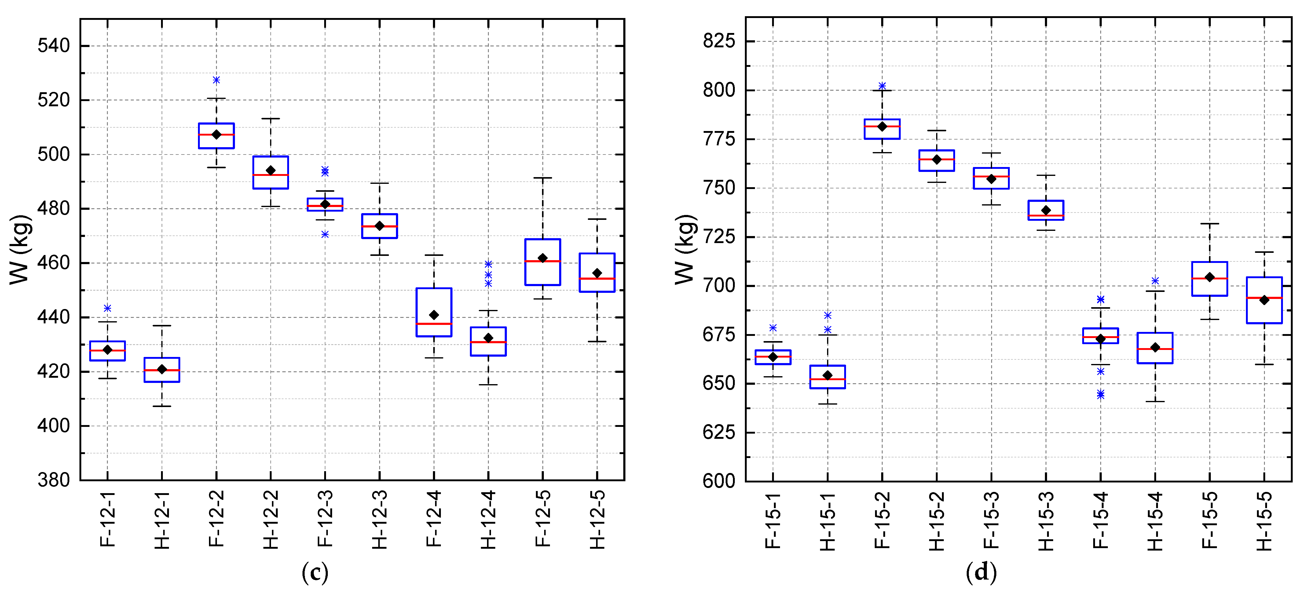
For the modified Fan typology, the results obtained through optimization indicate that for 6 m long trusses, the minimum objective functions varied between 112.96 kg and 170.40 kg, and for 9 m trusses, the minimum objective function varied between 238.12 kg and 301.21 kg. For 12 m long trusses, the minimum objective function values ranged from 417.53 kg to 527.46 kg. Finally, for 15 m long trusses, the minimum values of the objective function ranged between 644.02 kg and 802.28 kg.

For the Howe typology, the results obtained through optimization indicate that for 6 m long trusses, the minimum objective functions varied between 112.57 kg and 154.38 kg, and for 9 m trusses, the minimum objective function varied between 230.40 kg and 297.67 kg. For 12 m long trusses, the minimum objective function values ranged from 407.28 kg to 513.22 kg. Finally, for 15 m long trusses, the minimum values of the objective function ranged from 639.66 kg to 779.43 kg.

The results indicate that species ID 01 and ID 04 presented the best results for the objective function for both truss typologies. Although the resistance to normal solicitation was considered an important factor in the choice of wood for truss construction, the density and modulus of elasticity also played a significant role in determining the minimum weight of the trusses.

It is noteworthy that for wood trusses, it is of utmost importance to consider multiple factors in addition to the normal stress strength in the choice of wood species and truss configuration. The results also highlight the effectiveness of the optimization approach in obtaining efficient and cost-effective design solutions.

After the optimization process, it was possible to obtain the values of the design variables for each joist, respecting the established constraints. The results obtained present a feasibility rate of 100%.

Table 17. Summary of the design variables (modified Fan truss), measured in mm.

Variable	$\overrightarrow{{\mathit{x}}_1}$(mm)		$\overrightarrow{{\mathit{x}}_2}$(mm)		$\overrightarrow{{\mathit{x}}_3}$(mm)		$\overrightarrow{{\mathit{x}}_3}$(mm)		$\overrightarrow{{\mathit{x}}_5}$(mm)
	b	h	b	h	b	h	b	h	b	h
F-6-1	63	175	63	150	50	115	50	175	50	125
F-6-2	75	200	100	160	50	125	50	125	50	150
F-6-3	125	160	125	175	63	115	50	115	63	160
F-6-4	125	200	125	225	75	115	50	125	50	150
F-6-5	50	175	50	200	50	115	63	125	75	125
F-9-1	75	200	63	225	50	115	50	125	50	150
F-9-2	100	175	125	175	63	115	50	160	50	150
F-9-3	125	200	175	150	100	75	50	125	63	150
F-9-4	63	160	63	200	50	125	63	125	50	115
F-9-5	63	250	63	300	75	75	50	160	50	125
F-12-1	150	150	125	200	63	115	50	115	50	160
F-12-2	150	200	175	175	75	115	63	125	50	125
F-12-3	50	150	50	150	50	115	50	125	75	115
F-12-4	63	160	63	200	50	115	50	125	50	175
F-12-5	100	150	63	250	63	115	50	150	63	115
F-15-1	125	160	100	200	75	75	50	125	63	160
F-15-2	50	115	50	150	50	115	63	125	50	115
F-15-3	50	200	63	150	75	75	100	75	75	150
F-15-4	63	225	63	200	75	75	50	160	100	150
F-15-5	100	175	100	160	100	75	63	125	75	160

summarizes the design variables obtained for the modified Fan truss, indicating that the size and minimum area constraints were respected.

From Table 17, it can be observed that several trusses reached the minimum dimension for the elements. Trusses F-6-2, F-6-4, F-6-5, and F-9-5 reached the minimum dimension for the bottom chords, and trusses F-6-2, F-6-4, and F-6-5 reached the minimum dimension for the top chords. For the diagonals, F-6-1, F-6-2, F-6-3, F-6-4, F-6-5, F-9-1, F-9-2, and F-9-4 reached the minimum dimension. For the secondary uprights, trusses F-6-1, F-6-4, F-9-1, F-9-2, F-9-3, F-9-4, F-12-1, F-12-2, F-12-3, F-12-4, F-12-5, F-15-1, F-15-2, and F-15-4 met the minimum dimension. And finally, for the main upright, trusses F-6-1, F-6-3, F-6-5, F-9-1, F-9-2, F-9-3, F-9-4, F-12-2, F-12-3, F-15-1, and F-15-3 met the minimum dimension.

Table 18. Summary of the design variables (Howe truss), measured in mm.

Variável	$\overrightarrow{{\mathit{x}}_1}$(mm)		$\overrightarrow{{\mathit{x}}_2}$(mm)		$\overrightarrow{{\mathit{x}}_3}$(mm)		$\overrightarrow{{\mathit{x}}_3}$(mm)		$\overrightarrow{{\mathit{x}}_5}$(mm)
	b	h	b	h	b	h	b	h	b	h
H-6-1	50	200	50	200	50	115	63	125	75	115
H-6-2	63	160	50	175	50	115	50	160	75	150
H-6-3	63	175	100	115	50	115	75	115	50	125
H-6-4	63	115	50	160	50	115	50	115	63	175
H-6-5	50	115	50	150	50	115	50	115	100	160
H-9-1	75	200	50	300	50	115	50	115	63	160
H-9-2	100	160	75	175	50	115	50	125	50	125
H-9-3	75	225	75	225	50	125	50	115	63	150
H-9-4	63	175	75	150	50	115	50	160	50	175
H-9-5	63	150	63	160	50	115	50	150	50	150
H-12-1	125	175	125	160	75	75	50	160	63	150
H-12-2	100	200	75	250	63	125	50	115	50	150
H-12-3	150	160	100	225	63	115	50	125	75	160
H-12-4	63	250	125	115	75	75	75	125	50	175
H-12-5	75	160	63	225	75	75	50	160	100	115
H-15-1	125	225	125	200	75	115	50	115	50	150
H-15-2	100	250	150	160	75	115	63	115	75	125
H-15-3	200	160	125	225	100	75	50	115	100	160
H-15-4	175	115	125	150	75	75	63	160	75	175
H-15-5	150	115	75	225	75	75	50	150	63	150

summarizes the design variables obtained for the Howe truss. As in the results presented for the modified Fan truss, the minimum dimension and area constraints were respected.

From Table 18, it can be observed that several trusses reached the minimum dimension for the elements. Trusses H-6-1 and H-6-5 reached the minimum dimension for the bottom chords, and trusses H-6-1, H-6-2, H-6-4, H-6-5, and H-9-1 reached the minimum dimension for the top chords. For the diagonals, trusses H-6-1, H-6-2, H-6-3, H-6-4, H-6-5, H-9-1, H-9-2, H-9-3, H-9-4, and H-9-5 met the minimum dimension. For the secondary uprights, trusses H-6-2, H-6-4, H-6-5, H-9-1, H-9-2, H-9-3, H-9-4, H-9-5, H-12-1, H-12-2, H-12-3, H-12-5, H-15-1, and H-15-3 met the minimum dimension. Finally, for the main upright, trusses H-6-3, H-9-2, H-9-4, H-9-5, H-12-2, H-12-4, and H-15-1 reached the minimum dimension.

Figure 12 presents the results of the convergence curves of the best responses obtained after 30 repetitions of the weight optimization process for modified Fan-type trusses with spans of 6 m, 9 m, 12 m, and 15 m for species ID 01, ID 02, ID 03, ID 04, and ID 05. Considering a tolerance ratio of 10-2, it is observed that convergence occurred at iteration 337, 559, 377, 364, and 339 for trusses F-6-1, F-6-2, F-6-3, F-6-4, and F-6-5, respectively. For the 9 m span trusses, convergence occurred at iteration 256, 441, 239, 482, and 418 for trusses F-9-1, F-9-2, F-9-3, F-9-4, and F-9-5, respectively. For the 12 m span trusses, convergence occurred at iteration 556, 392, 566, 106, and 504 for trusses F-12-1, F-12-2, F-12-3, F-12-4, and F-12-5, respectively. Finally, for the 15 m span trusses, convergence occurred at iteration 496, 508, 562, 264, and 589 for trusses F-15-1, F-15-2, F-15-3, F-15-4, and F-15-5, respectively.

Similarly, Figure 13 presents the results of the convergence curves for the Howe typology considering a tolerance rate of 10–2. Convergence occurred at iteration 369, 226, 211, 274, and 434 for the H-6-1, H-6-2, H-6-3, H-6-4, and H-6-5 trusses, respectively. For the 9 m span trusses, convergence occurred at iteration 587, 320, 390, 465, and 516 for trusses H-9-1, H-9-2, H-9-3, H-9-4, and H-9-5, respectively. For the 12 m span trusses, convergence occurred at iteration 548, 537, 473, 31, and 178 for trusses H-12-1, H-12-2, H-12-3, H-12-4, and H-12-5, respectively. Finally, for the 15 m span trusses, convergence occurred at iteration 419, 407, 509, 543, and 11 for trusses H-15-1, H-15-2, H-15-3, H-15-4, and H-15-5, respectively.

3.4.1. Comparison of Optimization Results

The purpose of this section is to visualize the data distribution and the statistical measures, such as the median, quartiles, and extreme values, allowing for a comparison of the results obtained in the optimization process through the box plot for each truss length and each truss typology.

Figure 14 presents the optimization results for the modified Fan and Howe trusses for truss lengths of 6 m, 9 m, 12 m, and 15 m. For each span analyzed, a box plot was generated for the modified Fan and the Howe typology together. In this type of graph, the middle line represents the median, the diamond-shaped point represents the mean, the box represents the interquartile range (IQR), the lines extending from the box represent the minimum and maximum values, and the asterisk-shaped points represent the outliers.

The results show that in general, the Howe typology presented lower results for the minimum objective function in comparison with the modified Fan typology. An exception occurred for the trusses with 6 m span for the species ID 02, ID 04, and ID 05. For these, the modified Fan typology presented lower results in comparison with the Howe typology.

It is also observed that for both truss typologies, the minimum objective function increased with the length of the truss. This indicates that it is necessary to consider truss length when designing a wooden truss in order to obtain efficient and economical design solutions.

In conclusion, the box plot analysis allowed for a comparison of the optimization results for different joist lengths and for different joist typologies. This analysis allowed us to identify the differences between the joist typologies and highlighted the importance of selecting suitable wood species and considering multiple factors in the design of wood joists.

The optimization approach proved to be an effective tool in obtaining efficient and economical design solutions for both truss typologies.

However, it is important to note that optimization results can be sensitive to input parameters and imposed constraints. Therefore, it is necessary to perform additional analysis and consider other performance metrics before making a final decision on the wood truss design.

For this analysis, the constraints obtained from the best optimization results were evaluated.

3.4.2. Constraints

The constraints include checks of the minimum dimension and area, limit slenderness, sizing in ULS considering the normal stresses in the bars, and sizing in SLS considering the deflection in the immediate and final condition. Figure 15 and Figure 16 present the design constraints obtained in the best simulations of the study for the modified Fan and Howe typologies, respectively.

Based on the analysis of the design solutions, it can be seen that all met the imposed constraints, which indicates that these solutions are feasible in terms of safety and performance. When evaluating Figure 15, it was observed that the investigated trusses presented negative values close to zero during the verification of the instantaneous deflection of the Serviceability Limit State (SLS) ($g_{85}$). This finding suggests that this constraint was one of the constraints that limited the optimization process, resulting in values between −10⁻³ and −10⁻².

In addition, other constraints were also limiting for some trusses. For example, the minimum dimensions were reached in the bottom chords ($g_{108}$ to $g_{112}$) of the F-6-2, F-6-4, F-6-5, and F-9-5 joists; for the upper chords ($g_{113}$ to $g_{119}$) of H trusses F-6-2, F-6-4, and F-6-5; for the diagonals ($g_{120}$ to $g_{123}$) of trusses F-6-1, F-6-2, F-6-3, F-6-4, F-6-5, F-9-1, F-9-2, and F-9-4; for the secondary uprights ($g_{124}$ and $g_{127}$) of the trusses F-6-1, F-6-4, F-9-1, F-9-2, F-9-3, F-9-4, F-12-1, F-12-2, F-12-3, F-12-4, F-12-5, F-15-1 F-15-2, and F-15-4; and for the main stem ($g_{128}$) of the trusses F-6-1, F-6-3, F-6-5, F-9-1, F-9-2, F-9-3, F-9-4, F-12-2, F-12-3, F-15-1 and F-15-3, resulting in constraints equal to zero.

Analyzing the design solutions in the Howe typology, it was verified that all met the imposed constraints. Figure 16 shows that the investigated trusses presented negative values close to zero during the verification of the instantaneous deflection of the Serviceability Limit State (SLS) ($g_{85}$). This finding suggests that the instantaneous deflection constraint was one of the factors that limited the optimization process, resulting in values between −10⁻³ and −10⁻².

In addition, other constraints were also limiting for some trusses. For example, the minimum dimensions were reached for the bottom chords ($g_{108}$ to $g_{112}$) of trusses H-6-1 and H-6-5; for the top chords ($g_{113}$ to $g_{119}$) of trusses H-6-1, H-6-2, H-6-4, H-6-5, and H-9-1; for the diagonals ($g_{120}$ to $g_{123}$) of trusses H-6-1, H-6-2, H-6-3, H-6-4, H-6-5, H-9-1, H-9-2, H-9-3, H-9-4, and H-9-5; for the secondary uprights ($g_{124}$ and $g_{127}$) of trusses H-6-2, H-6-4, H-6-5, H-9-1, H-9-2, H-9-3, H-9-4, H-9-5, H-12-1, H-12-2, H-12-3, H-12-5, H-15-1, and H-15-3; and for the main stem ($g_{128}$) of trusses H-6-3, H-9-2, H-9-4, H-9-5, H-12-2, H-12-4, and H-15-1, resulting in zero constraints.

In the ULS checks for both types, the slenderness ($g_1$ to $g_{21}$) and minimum area ($g_{108}$ to $g_{128}$) constraints in the bars did not result in values close or equal to zero, indicating that the design was not limited by these constraints, but by the displacement constraint in the SLS in the instantaneous condition. This constraint made it impossible to reduce the objective function.

It should be noted that the constraints imposed depend on the intended use of the timber truss and may vary according to the specific application. Therefore, it is necessary to carefully consider the application-specific constraints when designing a timber truss. In addition, it is important to remember that the choice of wood species can also affect the constraints imposed and therefore should be considered carefully.

In summary, analyzing the results of the constraints arising from the optimization process, it can be seen that the imposed constraints made it possible to obtain efficient and safe design solutions for wood trusses. However, it is important to carefully consider the application-specific constraints and to choose the wood species appropriately to obtain an efficient and safe design solution.

3.4.3. Evaluation of ULS Constraints

In order to evaluate the ability to distribute normal loads in the truss, analyses of the normal stress constraints were performed. These analyses were conducted taking into account combinations 1, 2, and 3 for the loaded bars.

The results of these analyses were calculated for the average ($\overline{x}$), the standard deviation ($\sigma$), and the 95% confidence interval (CI). These values are presented in

Table 19. Summary of ULS constraints.

Typology	$\overline{\mathit{x}}$	$\mathit{\sigma }$	CI	Typology	$\overline{\mathit{x}}$	$\mathit{\sigma }$	CI
F-6-1	−0.5783	0.2517	(−0.6501; −0.5064)	H-6-1	−0.5998	0.2544	(−0.6704; −0.5291)
F-6-2	−0.7008	0.1719	(−0.7726; −0.6290)	H-6-2	−0.7158	0.2012	(−0.7865; −0.6452)
F-6-3	−0.7770	0.1171	(−0.8488; −0.7051)	H-6-3	−0.7804	0.1253	(−0.8511; −0.7098)
F-6-4	−0.7846	0.1369	(−0.8564; −0.7127)	H-6-4	−0.8031	0.1400	(−0.8738; −0.7325)
F-6-5	−0.8310	0.1110	(−0.9029; −0.7592)	H-6-5	−0.8474	0.1139	(−0.9166; −0.7782)
F-9-1	−0.5459	0.1921	(−0.6059; −0.4860)	H-9-1	−0.5549	0.2307	(−0.6189; −0.4908)
F-9-2	−0.6709	0.1525	(−0.7308; −0.6109)	H-9-2	−0.6781	0.1747	(−0.7421; −0.6140)
F-9-3	−0.7483	0.0984	(−0.8082; −0.6883)	H-9-3	−0.7607	0.1175	(−0.8248; −0.6967)
F-9-4	−0.7682	0.1133	(−0.8282; −0.7083)	H-9-4	−0.7790	0.1340	(−0.8430; −0.7149)
F-9-5	−0.8106	0.1148	(−0.8705; −0.7506)	H-9-5	−0.8238	0.1032	(−0.8865; −0.7610)
F-12-1	−0.5156	0.1677	(−0.5693; −0.4619)	H-12-1	−0.5120	0.2263	(−0.5737; −0.4503)
F-12-2	−0.6664	0.1320	(−0.7202; −0.6127)	H-12-2	−0.6725	0.1595	(−0.7342; −0.6108)
F-12-3	−0.7357	0.0821	(−0.7894; −0.6819)	H-12-3	−0.7503	0.1148	(−0.8120; −0.6886)
F-12-4	−0.7628	0.1140	(−0.8165; −0.7090)	H-12-4	−0.7572	0.1310	(−0.8189; −0.6955)
F-12-5	−0.7979	0.1083	(−0.8517; −0.7442)	H-12-5	−0.8100	0.1001	(−0.8705; −0.7496)
F-15-1	−0.5025	0.1554	(−0.5522; −0.4527)	H-15-1	−0.5092	0.1955	(−0.5673; −0.4511)
F-15-2	−0.6404	0.1175	(−0.6901; −0.5906)	H-15-2	−0.6605	0.1567	(−0.7186; −0.6024)
F-15-3	−0.7327	0.0873	(−0.7825; −0.6829)	H-15-3	−0.7450	0.1204	(−0.8031; −0.6869)
F-15-4	−0.7303	0.0965	(−0.7801; −0.6805)	H-15-4	−0.7468	0.1314	(−0.8049; −0.6886)
F-15-5	−0.7968	0.1058	(−0.8465; −0.7470)	H-15-5	−0.7924	0.0960	(−0.8494; −0.7355)

for the modified Fan and Howe trusses, respectively. The 95% confidence interval indicates that there is a 95% probability that the true mean is within this interval.

The distribution of the results can be visualized by means of a box plot, as presented in Figure 17 and Figure 18 for the modified Fan and Howe trusses, respectively.

The results obtained are important to verify whether the loads are being properly distributed on the truss bars, ensuring that the structure supports the applied loads safely and efficiently. The analysis of the distribution of the results can also indicate the need for adjustments in the structure, aiming to improve its load-bearing capacity.

The value of the constraint indicates how close the normal stress is to the limit established by the standard. Therefore, the closer to zero the result of the constraint, the more stressed are the elements of the truss. Analyzing the results presented in Table 19, it is observed that the trusses composed by the ID 01 species present higher solicitation, indicating a more uniform distribution of normal stress loads. It was verified that the normal stresses acting on the lattice elements correlate with the characteristic strength parallel to the fibers in compression ($f_{c0,k}$) and in tensile ($f_{t0,k}$), following the pattern of mechanical strength of the species. Thus, the trusses with species of lower mechanical strength are under greater demand, whereas the trusses with species of higher mechanical strength under less demand. Thus, analyzing the average value of the normal stress constraints, it is possible to classify the trusses in descending order of demand according to the species used, with the ID 01 species trusses being under the most demand, followed by the ID 02, ID 03, ID 04, and ID 05 species, respectively. It is worth noting that for the Howe typology, the ID 03 and ID 04 species showed similar average values. In addition, they had similar maximum and minimum values.

In order to compare the mechanical performance of the typologies, Figure 17 and Figure 18 were combined into a single graph for each span analyzed, as shown in Figure 19.

From Figure 19, it is possible to observe that the two typologies present similar average values for these constraints.

However, when analyzing the maximum and minimum values of the constraints, it is possible to notice that the Howe truss typology presents a larger amplitude in relation to the modified Fan truss typology in most of the adopted conditions. This suggests that the Howe truss typology is able to distribute efforts more efficiently, resulting in more uniform values of normal stresses.

This analysis is important to understand the differences between the two truss typologies and to identify which one may be more suitable for a given application. In addition, the results obtained can be useful for the development of standards and guidelines related to the use of trusses in building structures.

To statistically evaluate the existence of significant differences between the means of the groups regardless of the ULS constraints, the Anderson–Darling (A-D) and the Multiple Comparison Test (M-C) were applied. The Anderson–Darling test is used to check the normality of the data, and the Multiple Comparison Test is used to check for equality of variances between groups. These tests were used to evaluate the differences between the sample means of the groups and to check whether there was enough variation between the groups to indicate that the differences in the means were not merely random.

The results of these tests are presented in

Table 20. Summary statistical results of ULS constraints for the trusses.

Typology	Span	p-Value			Turkey (Grouping)
		ANOVA	A-D	M-C	ID 01	ID 02	ID 03	ID 04	ID 05
Fan	6 m	0.001	0.068	0.132	A	AB	B	B	B
	9 m	0.001	0.271	0.433	A	B	BC	BC	C
	12 m	0.001	0.254	0.067	A	B	BC	BC	C
	15 m	0.001	0.302	0.126	A	B	BC	BC	C
Howe	6 m	0.001	0.107	0.071	A	AB	B	B	B
	9 m	0.001	0.758	0.374	A	AB	BC	BC	C
	12 m	0.001	0.481	0.054	A	B	BC	BC	C
	15 m	0.001	0.150	0.093	A	B	BC	BC	C

, allowing the existence of significant differences between the group means to be verified. This statistical analysis contributes to the understanding of the relationship between the wood species used in the lattices and their mechanical strength, allowing for the selection of more appropriate species for this type of application.

The statistical analysis presented in Table 20 shows statistically significant differences between the means of the groups in relation to the ULS constraints. The Anderson–Darling (A-D) test confirmed that the data had a normal distribution, and the Multiple Comparison Test (M-C) showed that there was enough variation between groups to justify the analysis. Thus, it was possible to identify the groups that had statistically significant differences in the means of the ULS constraints. In total, two groups were identified for the 6 m trusses, and three groups were identified for the 9 m, 12 m, and 15 m trusses.

3.4.4. Evaluation of SLS Constraints

Service Limit State (SLS) constraints are a fundamental part of structural design and construction, because they ensure that a structure is able to withstand the loads that will be applied to it throughout its service life without suffering excessive or unacceptable damage. These constraints include limitations on various aspects of the structure’s performance, such as deformation, vibration, and fatigue, and they are established according to applicable standards and regulations.

One of the key aspects of SLS constraints is that they directly influence the design and dimensioning of a structure. For example, the choice of materials to be used in the construction of a structure must consider the SLS constraints in order to ensure that the structure meets performance and safety requirements throughout its service life.

ABNT NBR 7190-1 [23], a Brazilian standard that establishes guidelines for the design of timber structures, establishes limit values for deflections, which are a measure of deformation that occurs in the structure. These limit values are differentiated between the immediate and final conditions of the structure. The immediate condition refers to the state of the structure during its construction and immediately after it is put into use, and the final condition refers to the structure after it has been subjected to all expected loads and aging but is still within its design life.

Therefore, it is essential that the analysis of the immediate and final conditions be performed properly to ensure that the structure meets the performance and safety requirements at all stages of its service life, from construction to daily use and aging. Figure 20 presents the constraints of the SLS, both in the immediate ($g_{85}$) and final ($g_{86}$) states, expressed as a percentage of the maximum allowable displacement in relation to the established limit, which is a safety measure that ensures that the structure can support the expected loads.

During the SLS analysis, it was verified that for the immediate condition of the structure, the loads were between 96.51% and 99.92% of the limit established by the standard. For the final SLS condition, the loads were between 27.30% and 28.84% of the established limit. Moreover, it is possible to observe that all the trusses presented values close to 100% in the SLS immediate deflection condition, which indicates that this restriction was one of the constraints that limited the optimization process.

These results indicate that the optimized structure presents a good capacity to support the expected loads throughout its service life. It is important to emphasize the relevance of considering the SLS constraints from the design phase to the operation of the structure, in order to guarantee that it is able to support the expected loads without compromising safety and durability. Moreover, the analysis of the results obtained for the immediate and final SLS conditions allows for a better understanding of the structure’s behavior over time, guiding possible interventions to ensure its safe and adequate operation. It is concluded, therefore, that the optimization of the structure was limited by the SLS in the immediate condition, but that its use throughout the service life is possible.

4. Conclusions

This paper seeks to compare different types of structures in order to determine the lowest wood consumption, considering the influence of using different native wood species. For this, the FA optimization algorithm was applied by means of structural analysis software programmed based on matrix analysis and the ABNT NBR 7190-1 [23] standard for sizing.

A simulation was performed on modified Fan and Howe truss typologies with spans of 6, 9, 12, and 15 m, considering different strength classes of native wood species.

The analysis of the results allowed for reaching the following conclusions:

• The optimization process was successful and can be applied to design problems for structural design.
• The serviceability conditions of the SLS were guaranteed, since the instantaneous and effective displacements were below the normative limits of L/300 and L/150, respectively.
• The SLS design constraints in the instantaneous condition were limiting for all trusses during the optimization process.
• Regarding the influence of the species, it was found that the lowest objective function was a result of the association of species with good properties of bulk density, resistance to normal load, and modulus of elasticity. Moreover, it was found that the distribution of efforts follows the pattern of strength of species, where the trusses with species of lower mechanical strength were under greater demand, whereas the trusses with species of higher mechanical strength were under less demand. Thus, the trusses were classified in descending order of demand according to the species used, with ID 01 and ID 02 species trusses being under the greatest demanded, followed by ID 03, ID 04, and ID 05 species.
• As for the comparison between the typologies, the Howe typology presented lower results for the objective function in relation to the modified Fan truss in most of the results.
• When analyzing the ULS constraints, both typologies presented similar results. However, when analyzing the maximum and minimum values of the constraints, it is possible to notice that the Howe truss typology presents a larger amplitude in relation to the modified Fan truss typology in most of the adopted conditions. This suggests that the Howe truss typology is able to distribute the efforts in a more efficient way, resulting in more uniform values of normal stresses.
• It was possible to identify the groups that presented statistically significant differences in relation to the means of the ULS constraints. In total, two groups were identified for the 6 m trusses, and three groups were identified for the 9 m, 12 m, and 15 m trusses.
• Regarding the SLS constraints, it was verified that for the immediate condition of the structure, the loads were between 96.51% and 99.92% of the limit established by the standard. For the final SLS condition, the loads were between 27.30% and 28.84% of the established limit.

In summary, the study presents evidence that wood is a viable and sustainable choice for building systems, especially in structural applications such as trusses. The characterization of the properties of the wood species used in the study allowed for a more accurate analysis of the trusses’ performance, and the use of matrix analysis methods and swarm intelligence optimization algorithms allowed for an accurate evaluation of the internal forces and nodal displacements in the trusses, in addition to the minimization of the structure weight.

The results obtained indicate that trusses designed with different wood species present distinct behaviors, and this makes it possible to choose the most appropriate species for each specific application, considering its mechanical properties. Moreover, the analysis of the constraints associated with immediate deflection highlights the importance of considering all constraints in the design of timber structures.

Therefore, the use of wood in building systems, especially in trusses, is a sustainable and viable alternative that can contribute to a reduction in the environmental impact of civil construction.

References

1. Batista, M.; Amorim, A.; Silva, D.A.L.; Aquino, V.B.D.M.; Lahr, F.A.R.; Christoforo, A.L. Representativeness of the fiber parallel elasticity modulus value referring to the Brazilian standard C40 strength class in the design of timber structures. Cienc. Rural 2023, 53, e20210289. [Google Scholar] [CrossRef]
2. Pigozzo, J.C.; Arroyo, F.N.; Christoforo, A.L.; de Almeida, D.H.; Junior, C.C.; Lahr, F.A.R. Design and Execution of Wood-concrete Deck Bridge. Curr. J. Appl. Sci. Technol. 2018, 28, 1–10. [Google Scholar] [CrossRef]
3. Qin, R.; Zhou, A.; Chow, C.L.; Lau, D. Structural performance and charring of loaded wood under fire. Eng. Struct. 2021, 228, 111491. [Google Scholar] [CrossRef]
4. Fraga, I.F. Influência Dos Modelos Idealizados de Ligações No Dimensionamento de Treliças Planas de Madeira. Master’s Thesis, Universidade Federal do Rio Grande do Sul, São Carlos, Brazil, 2020. [Google Scholar]
5. Cavalheiro, R.S.; Almeida, D.H.; Christoforo, A.L.; Lahr, F.A.R. Density as Estimator of Shrinkage for Some Brazilian Wood Species. Int. J. Mater. Eng. 2016, 6, 107–112. [Google Scholar] [CrossRef] [Green Version]
6. Ramage, M.H.; Burridge, H.; Busse-Wicher, M.; Fereday, G.; Reynolds, T.; Shah, D.U.; Wu, G.; Yu, L.; Fleming, P.; Densley-Tingley, D.; et al. The wood from the trees: The use of timber in construction. Renew. Sustain. Energy Rev. 2017, 68, 333–359. [Google Scholar] [CrossRef]
7. Calil Júnior, C.; Dias, A.A. Utilização da madeira em construções rurais. Rev. Bras. Eng. Agríc. Ambient. 1997, 1, 71–77. [Google Scholar] [CrossRef]
8. Kromoser, B.; Reichenbach, S.; Hellmayr, R.; Myna, R.; Wimmer, R. Circular economy in wood construction—Additive manufacturing of fully recyclable walls made from renewables: Proof of concept and preliminary data. Constr. Build. Mater. 2022, 344, 128219. [Google Scholar] [CrossRef]
9. Amorim, S.T.A.; Mantilla, J.N.R.; Carrasco, E.V.M. A madeira laminada cruzada: Aspectos tecnológicos, construtivos e de dimensionamento. Matéria 2018, 22, 1–7. [Google Scholar] [CrossRef] [Green Version]
10. Andrade Junior, J.R.; Almeida, D.H.; Almeida, T.H.; Christoforo, A.L.; Stamato, G.C.; Lahr, F.A. Avaliação das estruturas de cobertura em madeira de um galpão de estoque de produtos químicos. Ambiente Construído 2014, 14, 75–85. [Google Scholar] [CrossRef] [Green Version]
11. Chen, Y.; Guo, W. Nondestructive Evaluation and Reliability Analysis for Determining the Mechanical Properties of Old Wood of Ancient Timber Structure. Bioresources 2017, 12, 2310–2325. [Google Scholar] [CrossRef] [Green Version]
12. De Araujo, V.A.; Cortez-Barbosa, J.; Gava, M.; Garcia, J.N.; De Souza, A.J.D.; Savi, A.F.; Morales, E.; Molina, J.C.; Vasconcelos, J.S.; Christoforo, A.L.; et al. Classification of Wooden Housing Building Systems. Bioresources 2016, 11, 7889–7901. [Google Scholar] [CrossRef] [Green Version]
13. Masoomi, H.; Ameri, M.R.; van de Lindt, J.W. Wind Performance Enhancement Strategies for Residential Wood-Frame Buildings. J. Perform. Constr. Facil. 2018, 32, 04018024. [Google Scholar] [CrossRef]
14. Kirkham, W.J.; Gupta, R.; Miller, T.H. State of the Art: Seismic Behavior of Wood-Frame Residential Structures. J. Struct. Eng. 2014, 140, 04013097. [Google Scholar] [CrossRef] [Green Version]
15. Wherry, G.; Buehlmann, U. Product Life Cycle of the Manufactured Home Industry. Bioresources 2014, 9, 6652–6668. [Google Scholar] [CrossRef] [Green Version]
16. FAO. Global Forest Resources Assessment 2020: Main Report; Food and Agriculture Organization—FAO: Rome, Italy, 2020; ISBN 978-92-5-132974-0. [Google Scholar]
17. ABNT NBR 7190; Projeto de Estruturas de Madeira. Associação Brasileira de Normas Técnicas—ABNT: Rio de Janeiro, Brazil, 2022.
18. de Santana, A.C.; de Santana, L.; dos Santos, M.A.S. Influência do desmatamento no mercado de madeira em tora da região Mamuru-Arapiuns, Sudoeste do Pará. RCA 2011, 54, 44–53. [Google Scholar] [CrossRef]
19. Moreira, J.M.M.P.; Simioni, F.J.; De Oliveira, E.B. De Importância e Desempenho Das Florestas Plantadas No Contexto Do Agronegócio Brasileiro. Floresta 2017, 47, 85–94. [Google Scholar] [CrossRef] [Green Version]
20. Dos Santos, H.F.; de Moraes, M.H.M.; de Oliveira, I.A.; de Freitas, L.; Aquino, V.B.D.M.; Menezes, I.S.; Fraga, I.F.; Lahr, F.A.R.; Mascarenhas, F.J.R.; Filho, F.M.D.A.; et al. Influence of the Harvesting Region on Batch Homogeneity of Ipe Wood (Tabebuia sp.) Based on Its Physical and Mechanical Properties. Forests 2022, 13, 1385. [Google Scholar] [CrossRef]
21. Ter Steege, H.; Prado, P.I.; de Lima, R.A.F.; Pos, E.; Coelho, L.d.S.; Filho, D.d.A.L.; Salomão, R.P.; Amaral, I.L.; Matos, F.D.d.A.; Castilho, C.V.; et al. Biased-corrected richness estimates for the Amazonian tree flora. Sci. Rep. 2020, 10, 10130. [Google Scholar] [CrossRef]
22. Calil Júnior, C.; Lahr, F.A.R.; Dias, A.A.; Martins, G.C.A. Estruturas de madeira: Projetos, Dimensionamento e Exemplos de Cálculo, 1st ed.; Elsevier—GEN LTC: Rio de Janeiro, Brazil, 2019; ISBN 978-85-352-8680-9. [Google Scholar]
23. ABNT NBR 7190-1; Projeto de Estruturas de Madeira. Parte 1: Critérios de Dimensionamento. Associação Brasileira de Normas Técnicas—ABNT: Rio de Janeiro, Brazil, 2022.
24. European Committee for Standardization. Eurocode 5: Design of Timber Structures—Part 1-1: General—Common Rules and Rules for Buildings; BSI: Bruxelas, Bélgica, 2004. [Google Scholar]
25. Franck Filho, F.H. Seleção de Espécies Arbóreas Nativas Da Região Sul Do Brasil Para Reflorestamento E Emprego NA Arquitetura E No Design. Master’s Thesis, Universidade Federal do Rio Grande do Sul, Porto Alegre, Brazil, 2005. [Google Scholar]
26. Giglio, T.G.F.; Barbosa, M.J. Aplicação de métodos de avaliação do desempenho térmico para analisar painéis de vedação em madeira. Ambiente Construído 2006, 6, 91–103. [Google Scholar]
27. Kim, H.-S.; Park, Y.-S.; Yang, M.-K.; Lee, M.-H.; Kim, J.-Y. Initial Shape Design of Space Truss Structure using Density Method. J. Korean Assoc. Spat. Struct. 2010, 10, 59–66. [Google Scholar]
28. Lemonge, A.C.; Carvalho, J.P.; Hallak, P.H.; Vargas, D. Multi-objective truss structural optimization considering natural frequencies of vibration and global stability. Expert Syst. Appl. 2021, 165, 113777. [Google Scholar] [CrossRef]
29. Moraes, M.H.M.; Fraga, I.F.; Pereira Junior, W.M.; Christoforo, A.L. Comparative Analysis of the Mechanical Performance of Timber Trusses Structural Typologies Applying Computational Intelligence. Rev. Árvore 2022, 46, e4604. [Google Scholar] [CrossRef]
30. Mayencourt, P.; Mueller, C. Hybrid analytical and computational optimization methodology for structural shaping: Material-efficient mass timber beams. Eng. Struct. 2020, 215, 110532. [Google Scholar] [CrossRef]
31. Pech, S.; Kandler, G.; Lukacevic, M.; Füssl, J. Metamodel assisted optimization of glued laminated timber beams by using metaheuristic algorithms. Eng. Appl. Artif. Intell. 2019, 79, 129–141. [Google Scholar] [CrossRef]
32. Schietzold, F.N.; Graf, W.; Kaliske, M. Multi-Objective Optimization of Tree Trunk Axes in Glulam Beam Design Considering Fuzzy Probability-Based Random Fields. ASCE-ASME J. Risk Uncert. Engrg. Sys. Part B Mech. Engrg. 2021, 7, 020913. [Google Scholar] [CrossRef]
33. Mam, K.; Douthe, C.; Le Roy, R.; Consigny, F. Shape optimization of braced frames for tall timber buildings: Influence of semi-rigid connections on design and optimization process. Eng. Struct. 2020, 216, 110692. [Google Scholar] [CrossRef]
34. Christoforo, A.L.; de Moraes, M.H.M.; Fraga, I.F.; Junior, W.M.P.; Lahr, F.A.R. Computational Intelligence Applied in Optimal Design of Wooden Plane Trusses. Eng. Agríc. 2022, 42, e20210123. [Google Scholar] [CrossRef]
35. Villar, J.R.; Vidal, P.; Fernández, M.S.; Guaita, M. Genetic algorithm optimisation of heavy timber trusses with dowel joints according to Eurocode 5. Biosyst. Eng. 2016, 144, 115–132. [Google Scholar] [CrossRef]
36. Villar-García, J.R.; Vidal-López, P.; Rodríguez-Robles, D.; Guaita, M. Cost optimisation of glued laminated timber roof structures using genetic algorithms. Biosyst. Eng. 2019, 187, 258–277. [Google Scholar] [CrossRef]
37. Amaran, S.; Sahinidis, N.V.; Sharda, B.; Bury, S.J. Simulation optimization: A review of algorithms and applications. Ann. Oper. Res. 2016, 240, 351–380. [Google Scholar] [CrossRef] [Green Version]
38. Greenhalgh, D.; Marshall, S. Convergence Criteria for Genetic Algorithms. SIAM J. Comput. 2000, 30, 269–282. [Google Scholar] [CrossRef]
39. Parsopoulos, K.E.; Vrahatis, M.N. Recent approaches to global optimization problems through Particle Swarm Optimization. Nat. Comput. 2002, 1, 235–306. [Google Scholar] [CrossRef]
40. Lin, M.-H.; Tsai, J.-F.; Yu, C.-S. A Review of Deterministic Optimization Methods in Engineering and Management. Math. Probl. Eng. 2012, 2012, 756023. [Google Scholar] [CrossRef] [Green Version]
41. Segovia-Hernández, J.G.; Hernández, S.; Petriciolet, A.B. Reactive distillation: A review of optimal design using deterministic and stochastic techniques. Chem. Eng. Process. Process Intensif. 2015, 97, 134–143. [Google Scholar] [CrossRef]
42. Huang, C.; El Hami, A.; Radi, B. Metamodel-based inverse method for parameter identification: Elastic–plastic damage model. Eng. Optim. 2017, 49, 633–653. [Google Scholar] [CrossRef]
43. De Souza, R.R.; Miguel, L.F.F.; Lopez, R.H.; Miguel, L.F.F.; Torii, A.J. A procedure for the size, shape and topology optimization of transmission line tower structures. Eng. Struct. 2016, 111, 162–184. [Google Scholar] [CrossRef]
44. Issa, M.V.S. On the Accuracy and Efficiency of Cross-Entropy Method for Structural Optimization. Master’s Thesis, Universidade do Estado do Rio de Janeiro, Faculdade de Engenharia, Rio de Janeiro, Brazil, 2019. [Google Scholar]
45. Blum, C.; Roli, A. Metaheuristics in combinatorial optimization: Overview and Conceptual Comparison. ACM Comput. Surv. 2003, 35, 268–308. [Google Scholar] [CrossRef]
46. Ng, K.; Lee, C.; Chan, F.T.; Lv, Y. Review on meta-heuristics approaches for airside operation research. Appl. Soft Comput. 2018, 66, 104–133. [Google Scholar] [CrossRef]
47. Gandomi, A.H.; Yang, X.-S.; Alavi, A.H. Mixed variable structural optimization using Firefly Algorithm. Comput. Struct. 2011, 89, 2325–2336. [Google Scholar] [CrossRef]
48. Lieu, Q.X.; Do, D.T.; Lee, J. An adaptive hybrid evolutionary firefly algorithm for shape and size optimization of truss structures with frequency constraints. Comput. Struct. 2018, 195, 99–112. [Google Scholar] [CrossRef]
49. Pereira, L.L.M.; Santos, D.C.; Moraes, M.H.M.; Filho, G.M.G.; Junior, E.M.A.; Junior, W.M.P.; Dantas, M.J.P. Estudo de Sensibilidade do Algoritmo de Colônia de Vagalumes para um Problema de Engenharia Envolvendo Dimensionamento de Treliças. Tend. Mat. Apl. Comput. 2020, 21, 583. [Google Scholar] [CrossRef]
50. Kromoser, B.; Braun, M.; Ortner, M. Construction of All-Wood Trusses with Plywood Nodes and Wooden Pegs: A Strategy towards Resource-Efficient Timber Construction. Appl. Sci. 2021, 11, 2568. [Google Scholar] [CrossRef]
51. Jelusic, P.; Kravanja, S. Optimal design of timber-concrete composite floors based on the multi-parametric MINLP optimization. Compos. Struct. 2017, 179, 285–293. [Google Scholar] [CrossRef]
52. Šilih, S.; Kravanja, S.; Premrov, M. Shape and discrete sizing optimization of timber trusses by considering of joint flexibility. Adv. Eng. Softw. 2010, 41, 286–294. [Google Scholar] [CrossRef]
53. Kuri-Morales, A.F.; Gutiérrez-García, J. Penalty Function Methods for Constrained Optimization with Genetic Algorithms: A Statistical Analysis. In MICAI 2002: Advances in Artificial Intelligence; Coello Coello, C.A., de Albornoz, A., Sucar, L.E., Battistutti, O.C., Eds.; Lecture Notes in Computer Science; Springer: Berlin/Heidelberg, Germany, 2002; Volume 2313, pp. 108–117. ISBN 978-3-540-43475-7. [Google Scholar]
54. Yeniay, Ö. Penalty Function Methods for Constrained Optimization with Genetic Algorithms. Math. Comput. Appl. 2005, 10, 45–56. [Google Scholar] [CrossRef] [Green Version]
55. Yang, X.-S. Nature-Inspired Metaheuristic Algorithms; Luniver Press: Frome, UK, 2008; ISBN 978-1-905986-10-1. [Google Scholar]
56. Wang, H.; Wang, W.; Zhou, X.; Sun, H.; Zhao, J.; Yu, X.; Cui, Z. Firefly algorithm with neighborhood attraction. Inf. Sci. 2017, 382–383, 374–387. [Google Scholar] [CrossRef]
57. Hsu, C.S. A discrete method of optimal control based upon the cell state space concept. J. Optim. Theory Appl. 1985, 46, 547–569. [Google Scholar] [CrossRef]
58. ABNT NBR ISO 3179; Madeira Serrada de Coníferas—Dimensões Nominais. Associação Brasileira de Normas Técnicas—ABNT: Rio de Janeiro, Brazil, 2011.
59. ABNT NBR 7190-3; Métodos de Ensaio Para Corpos de Prova Isentos de Defeitos Para Madeiras de Florestas Nativas. Associação Brasileira de Normas Técnicas—ABNT: Rio de Janeiro, Brazil, 2022.
60. ABNT NBR 6120; Ações Para o Cálculo de Estruturas de Edificações. Associação Brasileira de Normas Técnicas—ABNT: Rio de Janeiro, Brazil, 2019.
61. ABNT NBR 6123; Forças Devidas Ao Vento Em Edificações. Associação Brasileira de Normas Técnicas—ABNT: Rio de Janeiro, Brazil, 1988.
62. ABNT NBR 8681; Ações e Segurança Nas Estruturas—Procedimento. Associação Brasileira de Normas Técnicas—ABNT: Rio de Janeiro, Brazil, 2003.
63. Telha São Carlos Catálogo de Telhas São Carlos. Available online: https://telhasaocarlos.com.br/wp-content/uploads/2019/04/CatalogoTelhaSaoCarlos_2019-compactado.pdf (accessed on 22 November 2022).
64. ABNT NBR 5738; Concreto—Procedimento Para Moldagem e Cura de Corpos de Prova. Associação Brasileira de Normas Técnicas—ABNT: Rio de Janeiro, Brazil, 2015.
65. Miyoshi, Y.; Kojiro, K.; Furuta, Y. Effects of density and anatomical feature on mechanical properties of various wood species in lateral tension. J. Wood Sci. 2018, 64, 509–514. [Google Scholar] [CrossRef]
66. ABNT NBR 7190; Projeto de Estruturas de Madeira. Associação Brasileira de Normas Técnicas—ABNT: Rio de Janeiro, Brazil, 1997.
67. Lahr, F.A.R.; Arroyo, F.N.; De Almeida, T.H.; Filho, F.M.D.A.; Mendes, I.S.; Christoforo, A.L. Full Characterization of Erisma uncinatum Warm Wood Specie. Int. J. Mater. Eng. 2016, 6, 147–150. [Google Scholar] [CrossRef] [Green Version]
68. Teixeira, J.N.; Wolenski, A.R.V.; Aquino, V.B.D.M.; Panzera, T.H.; Silva, D.A.L.; Campos, C.I.; Silva, S.A.M.; Lahr, F.A.R.; Christoforo, A.L. Influence of provenance on physical and mechanical properties of Angelim-pedra (Hymenolobium petraeum Ducke.) wood species. Eur. J. Wood Wood Prod. 2021, 79, 1241–1251. [Google Scholar] [CrossRef]
69. Lahr, F.A.R.; Christoforo, A.L.; da Silva, C.E.G.; Junior, J.R.d.A.; Pinheiro, R.V. Avaliação de Propriedades Físicas e Mecânicas de Madeiras de Jatobá (Hymenaea stilbocarpa hayne) Com Diferentes Teores de Umidade e Extraídas de Regiões Distintas. Rev. Árvore 2016, 40, 147–154. [Google Scholar] [CrossRef] [Green Version]
70. Da Silva, C.E.G.; De Almeida, D.H.; De Almeida, T.H.; Chahud, E.; Branco, L.A.M.N.; Campos, C.I.; Lahr, F.A.R.; Christoforo, A.L. Influence of the Procurement Site on Physical and Mechanical Properties of Cupiúba Wood Species. Bioresources 2018, 13, 4118–4131. [Google Scholar] [CrossRef]
Figure 1. Wood in roofing systems.
Buildings 13 01946 g001
Figure 2. Parallel chord trusses: (a) Brown truss, (b) Howe truss, (c) K truss, and (d) Pratt truss.
Buildings 13 01946 g002
Figure 3. Trapezoidal trusses: (a) Fan truss, (b) Howe truss, (c) Pratt truss, and (d) parallel chord truss.
Buildings 13 01946 g003
Figure 4. Triangular trusses: (a) modified Fan Truss, (b) Howe Truss, (c) Pratt Truss, and (d) scissor Truss.
Buildings 13 01946 g004
Figure 5. Types of optimizations: (a) size optimization, (b) geometric optimization, and (c) topological optimization.
Buildings 13 01946 g005
Figure 6. Process flowchart of the FA algorithm.
Buildings 13 01946 g006
Figure 7. Trusses and their design variables: (a) modified Fan truss, (b) Howe truss, and (c) design variables.
Buildings 13 01946 g007
Figure 8. Shed dimensions.
Buildings 13 01946 g008
Figure 9. Wind loads ( w k ) on the roof of the sheds: (a) Type 1, (b) Type 2, (c) Type 3, and (d) Type 4.
Buildings 13 01946 g009
Figure 10. Box plot of the penalized objective function W of the modified Fan trusses as a function of span: (a) 6 m, (b) 9 m, (c) 12 m, and (d) 15 m.
Buildings 13 01946 g010
Figure 11. Box plot of the penalized objective function W of the Howe trusses as a function of span: (a) 6 m, (b) 9 m, (c) 12 m, and (d) 15 m.
Buildings 13 01946 g011
Figure 12. Box plot of the penalized objective function W of the modified Fan trusses as a function of span: (a) 6 m, (b) 9 m, (c) 12 m, and (d) 15 m.
Buildings 13 01946 g012aBuildings 13 01946 g012b
Figure 13. Box plot of the penalized objective function W for Howe trusses as a function of span: (a) 6 m, (b) 9 m, (c) 12 m, and (d) 15 m.
Buildings 13 01946 g013aBuildings 13 01946 g013b
Figure 14. Comparative box plot of the penalized objective function (W): (a) 6 m, (b) 9 m, (c) 12 m, and (d) 15 m.
Buildings 13 01946 g014aBuildings 13 01946 g014b
Figure 15. Constraints (g) for spans 6, 9, 12, and 15 m for the modified Fan typology: (a) 6 m, (b) 9 m, (c) 12 m, and (d) 15 m.
Buildings 13 01946 g015
Figure 16. Constraints (g) for spans 6, 9, 12, and 15 m for the modified Fan typology: (a) 6 m, (b) 9 m, (c) 12 m, and (d) 15 m.
Buildings 13 01946 g016aBuildings 13 01946 g016b
Figure 17. Box plot of the ULS constraints (g) for the modified Fan typology: (a) 6 m, (b) 9 m, (c) 12 m, and (d) 15 m.
Buildings 13 01946 g017aBuildings 13 01946 g017b
Figure 18. Box plot of ULS constraints (g) for the Howe typology: (a) 6 m, (b) 9 m, (c) 12 m, and (d) 15 m.
Buildings 13 01946 g018
Figure 19. Box plot of ULS constraints (g) for the trusses: (a) 6 m, (b) 9 m, (c) 12 m, and (d) 15 m.
Buildings 13 01946 g019
Figure 20. Box plot of the SLS constraints (g): (a) 6 m, (b) 9 m, (c) 12 m, and (d) 15 m.
Buildings 13 01946 g020