How Building Energy Use Reacted to Variable Occupancy Pre- and Post- COVID-19 Pandemic—Sensitivity Analysis of 35 Commercial Buildings in Canada

Abstract

The COVID-19 pandemic and global shutdown and work-from-home order for non-essential businesses and employees led to a substantial decline in energy usage in the commercial building sector. However, the magnitude of decline was not equivalent to what would be expected for unoccupied spaces. The energy performance of low/unoccupied commercial buildings, particularly in the context of new minimum requirements to maintain indoor air quality, is an intriguing research question. In this study, we developed a numerical model that measures electricity usage sensitivity to occupancy (ESTO) where we compare the business-as-usual energy performance with unoccupied energy performance. Two years of COVID-time (in addition to a pre-COVID control year) hourly energy use (electricity (plug loads, lighting, and fans), heating, and cooling) using data from 35 commercial buildings (i.e., buildings with HVAC and other building systems typical of commercial rather than residential buildings) are analyzed to quantify those changes. A change point model is used to assess thermal load intensities, change point temperature, and off-season unoccupied baseloads. Finally, we suggest a generic framework for building scoring based on selected performance parameters. Results indicate that the suggested scoring system is robust and replicable and is reliable for ranking buildings within a given portfolio from best- to worst- performing, thus prioritizing buildings that are best candidates for retrofits.

1. Introduction

When the global lockdown took place because of the COVID-19 pandemic, all non-essential commercial activities were shut down and the majority of office workers began working from home. As a result, a considerable change in occupancy-driven energy use was observed in commercial buildings. The International Energy Agency [1] reported a drop in energy demand of 20% following the global lockdown order in March 2020 [2]. Even smart buildings were not programmed to adapt to sudden, long-term gaps in occupancy. Instead, standard, static schedules were followed for building operations. Consequently, building operators continued to follow these schedules during the COVID-19 lockdown, which lasted for approximately two years, and, as a result, avoidable building energy waste was observed during the lockdown period. Now that the world is recovering from the pandemic and most employees have returned to on-site work, it is critical to consider variable occupancy scenarios going forward. Smart buildings should adapt to partial- to no-occupancy scenarios in order to avoid energy waste, especially during extended unoccupied periods. Despite the fact that as of 1 May 2023, the UN WHO has declared an end to COVID-19 as a public health emergency [3], allowing most countries to return to routine activities as they were known before COVID-19, many governments and private sector employers have allowed flexible work schedules for their employees. In the present day, hybrid, telework, fully on-site, compressed week, as well as flexible hours have become popular work arrangements. Consequently, from the building operations viewpoint, the prediction of occupant-driven energy consumption has been associated with uncertainties, much greater than the uncertainty levels observed in the past. The research presented in this paper sheds light on the criticality of integrating occupant-centric optimization of building operations into new and existing buildings, for their ability to adapt to dynamic operations going forward [4]. Previous studies conducted on the implications of the COVID-19 pandemic on energy demand have primarily focused on the quantification of those implications, whether historically (within the affected time period) or in the near future (such as predicting the year-ahead scenario), where multiple approaches including baselining, multi-linear regression, simulation, and advanced machine learning techniques were deployed.

In this current study, we aim to utilize the lessons learned from (a) the unoccupied building energy performance behavior (which represents the no-occupancy scenario) and (b) the typical occupancy scenario pre-pandemic, in order to predict variable occupancy scenarios moving forward. In addition, from the research findings, we aim to explore the capability of identifying poor performing building components and prioritizing buildings that require retrofits the most. Thus, this research aims to develop a framework to (1) quantify the energy performance of unoccupied commercial buildings in Canada, relative to their respective fully-occupied energy performance; (2) assess the sensitivity of building energy consumption to occupancy and outdoor temperature, given that occupancy data are unavailable (alternatively, using a relative occupancy metric); and (3) assign a building performance scorecard based on multiple performance criteria.

Further material is divided into several parts. Thus, Section 2 summarizes the published literature on quantification of the implications of the COVID-19 pandemic on energy use at municipal, national, and international levels, identifying existing literature gaps and research objectives. Section 3 presents materials and methods, describing the research framework, methodology, and data description. Section 4 discusses the research findings. Section 5 presents the framework for ranking the energy performance of buildings within a given portfolio. Section 6 presents a discussion and interpretation of the results. Finally, Section 7 concludes the paper findings and suggests future directions.

2. Literature Review

The COVID-19 pandemic disrupted economies worldwide [5]. In order to contain the spread of the COVID-19 virus, various measures were taken, including partial or complete lockdowns, curfews, restrictions on public gatherings, and shutdowns of businesses deemed to be non-essential [6]. In 2020, after COVID-19 was declared a global pandemic by the WHO, researchers were motivated to use new trends in electricity usage to predict future demand, but had limited information on the long-term socio-economic impacts of the pandemic and the duration of those impacts. Ref. [7] predicted annual energy savings in kindergartens, schools, apartments, and townhouses in Norway using data from March 2020 to December 2020. They found that if unoccupied educational facilities followed the nighttime and weekend schedules during weekdays, annual electricity usage would drop by a third. On the other hand, if residential buildings operated in a work-from-home context, the annual electricity demand would increase by 27% and 1.3% for apartments and townhouses, respectively. Ref. [5] found that electricity consumption and nighttime lighting can act as an indicator for measuring economic activity in India. In India, a national lockdown took place on 25 March 2020, where energy consumption declined by more than 25% in the short-term, and then recovered gradually over the long term as the restrictions were eased step-by-step. In the past, methods employing electricity consumption and nighttime lighting intensity have been deployed to track economic activity and to improve India’s GDP national account estimates [8]. The COVID-19 infection rate also played a role in energy usage. A higher infection rate was linked to a decline in nighttime lighting intensity [5].

Some unexpected energy performance behaviors were also observed. Despite the criticality of hospital operations during the COVID-19 pandemic, especially during the initial response to the virus in March and April 2020, Ref. [6] concluded that hospital electricity demand during this period decreased relative to the same time period in 2019. They elaborated that, even though hospitals were overwhelmed by the number of patients requiring critical care depending primarily on electricity supply (such as electric ventilators and inhalers), some non-urgent programmed surgery and outpatient consultations had been cancelled or postponed, leading to an overall reduction in hospital electricity usage of 19.49%. Ref. [9] also found that the stringency of lockdown measures and mobility, especially for retail and recreation centers, had a direct impact on deviation in electricity demand. Ref. [10] studied the electricity performance of 27 commercial smart buildings in the National Capital Region in Canada during the two years following the COVID-19 pandemic lockdown. Their study concluded an average reduction of 10% in commercial smart buildings during the first year following the COVID-19 pandemic lockdown order, where the change rate was non-uniform across different building archetypes. For context, in Ontario, the share of annual electricity demand for the building sector is 36%, 29%, and 31% for commercial, industrial, and residential buildings, respectively. Refs. [11,12] studied the effects of the COVID-19 pandemic on electricity consumption at the utility/customer-class scale in the United States—specifically, the shift in electricity usage between the commercial and residential sectors. They addressed the questions of “when, where, and how we use electricity” during the pandemic lockdown.

Conversely, the occupation of residential buildings rose during the lockdown order, due to occupants working and conducting many other activities from home. While it is typically expected that residential energy demand would increase during lockdown, Ref. [13] conducted various energy simulation scenarios in Sweden, concluding that space heating demand went down from 27.4 kWh/m² under normal occupancy schedules, to 19.9 kWh/m² under a 24-h full occupancy for an entire year, due to the increase in internal heat gains. Ref. [14] studied the effects of the COVID-19 pandemic on energy (electricity, hot water, and space heating) consumption in Canadian social housing at two levels: total usage and daily patterns. They concluded that during mid-day, electricity usage and hot water usage increased by 46% and 103%, respectively, while space heating did not change compared to pre-COVID consumption. Ref. [14] stated that according to Google’s COVID-19 Community Mobility Reports, during the first month following the COVID-19 pandemic lockdown, occupation of residential buildings increased by 21%, whereas that of retail and recreation facilities dropped by 63%. Similarly, Ref. [15] studied the effects of the stay-at home order due to the COVID-19 pandemic on residential electricity usage in New York, U.S. Ref. [6] studied the effect of COVID-19 lockdown measures on electricity consumption and load patterns in Spain. Their analysis was carried out by comparing electrical demand during the COVID-19 lockdown period until end of April, 2020 (nearly 6 weeks) with the average electricity demand over the past 5 years (2015–2019). Weekday and weekend electrical demand declined by 14.53% and 10.62%, respectively. Ref. [16] studied how German and other European electrical grids reacted to the COVID-19 pandemic lockdown at a national level. Ref. [17] also studied the impacts of the COVID-19 pandemic on electrical demand in multiple European countries with varying levels of lockdown restriction, for example, Spain, Italy, Belgium, and the UK as countries with severe restrictions, and the Netherlands and Sweden as countries with less restrictive measures. Results indicated that during the week following the lockdown order, electricity consumption decreased by 25%, 17.7%, 15.6%, 14.2%, and 11.6% for Spain, Italy, Belgium, United Kingdom, and Netherlands, respectively, but also interestingly increased in Sweden by 2.1%. Ref. [18] studied trends in electrical load in Brazil during the COVID-19 pandemic by comparing demand before and after the pandemic lockdown order. A heterogeneous change across different regions in Brazil was reported, where the highest drop in electricity usage was observed in the South subsystem (19%), followed by the Southeast, Northeast, and North subsystems, with reductions of 15%, 14%, and 3%, respectively. Ref. [19] quantified the impacts of the COVID-19 pandemic on gas and electricity demands in China. Ref. [9] studied the global (with a sample of 58 countries) electricity market deviation during the eight-month period following the COVID-19 lockdown order. Ref. [20] investigated the impacts of the COVID-19 pandemic on the electrical grid of Great Britain, where demand was reduced by approximately 25%. The electricity load profile in Great Britain shows that during the initial response to the COVID-19 lockdown order, peak loads had the highest reduction (−20.31%) while base loads had the least reduction (−9.5%). In the State of Kuwait, during the COVID-19 pandemic lockdown, electrical power demand at the state level dropped by 17.6% during the full lockdown period, as compared to the predicted electrical power demand [21]. In Poland, it was found that offices and shopping centers had the most significant drop in electricity usage during the initial lockdown period, with a 15–23% reduction compared to the pre-pandemic usage. Refs. [22,23] shed light on the heterogeneity of variations in electric power demand during the COVID-19 pandemic, referring to the responses of the various U.S. states to the initial pandemic lockdown order. The variation is not only on the aggregate level, but also on the grid stress level, for example, peak demand, where some states indicated increased stress, less stress, or even no significant change. Ref. [11] found that during the initial stage of the COVID-19 pandemic (i.e., March 2020–June 2020), electricity demand in Canada dropped by 10% in Ontario, and about 5% in Alberta, British Columbia, and New Brunswick. In April 2020, electrical demand in the Province of Ontario dropped by 14% overall, and by 16% in Ottawa (the national capital of Canada) [24]. Ref. [9] classified the global initial response (decline) severity and recovery speed in electricity demand during the initial COVID-19 period (January–April 2020) and found that, in Ontario, the initial response fell under the “severe” category, while that of Alberta and British Columbia fell under the “mild” category; however, the speed of recovery for all three provinces was quick. Table 1 summarizes this literature review of the short-term deviation in electrical demand worldwide due to the pandemic lockdown order.

In conclusion, the electrical demand in the building sector at municipal, national and international levels had been clearly affected by the COVID-19 pandemic; this implies substantial socio-economic disruption, since energy demand is directly linked to people’s activities, in particular, work activities [25]. However, the extent and duration of disruption showed heterogeneity, depending on the building sector (e.g., housing, commercial, educational), degree of lockdown strictness, and spread of the virus, as well as behavioral aspects and protective measures applied in buildings (e.g., increased outdoor air intake, limited occupancy, mobility). Going forward, it is critical that while we prioritize health and safety in buildings by, for example, maximizing outdoor air intake, we do this in an energy-efficient manner with regard for climate change mitigation [16].

Table 1. Summary of short-term deviation in electricity demand due to the pandemic lockdown order.

Country	Short-Term Deviation (1–6 Months)
	Country-Wide	Commercial	Residential
India	−20 to −30% [5]
Spain	−13.5% [6], −25% [17]
Italy	−17.7% [17], −25% [6]
Belgium	−15.6 [17]
United Kingdom	−14.2 [17]
Netherlands	−11.6% [17]
Sweden	+2.1% [17]
Poland	−15 to −23% [22]
U.S.	−12% (except Florida) [26]	−9% (commercial), −11% (industrial) [12]	+6% [12]
Brazil	−3 to −19% [18]
Canada	−5% to −16% [24]	−10% [10]
Kuwait	−17.6% [21]

Table 1. Summary of short-term deviation in electricity demand due to the pandemic lockdown order.

Country	Short-Term Deviation (1–6 Months)
	Country-Wide	Commercial	Residential
India	−20 to −30% [5]
Spain	−13.5% [6], −25% [17]
Italy	−17.7% [17], −25% [6]
Belgium	−15.6 [17]
United Kingdom	−14.2 [17]
Netherlands	−11.6% [17]
Sweden	+2.1% [17]
Poland	−15 to −23% [22]
U.S.	−12% (except Florida) [26]	−9% (commercial), −11% (industrial) [12]	+6% [12]
Brazil	−3 to −19% [18]
Canada	−5% to −16% [24]	−10% [10]
Kuwait	−17.6% [21]

Research Gaps and Objectives

In this study, we complement the foundational work on the implications of the COVID-19 pandemic on energy usage by contributing to the following research objectives:

• Analyze the energy performance of 35 commercial smart buildings for 2 full years following the COVID-19 pandemic lockdown order on 16 March 2020, where 3 energy types are addressed (electricity (lighting, plug loads, and fans), district heating (steam or high temperature hot water), and district cooling (chilled water));
• Use change point model analysis to understand the heating and cooling load characteristics of buildings during the unoccupied period;
• Perform a black-box sensitivity analysis on the effects of occupancy levels on electricity usage, taking the COVID-19 stay-home period as a reference for electricity performance with no occupancy, and the pre-COVID period as a reference for business-as-usual electrical performance;
• Propose electricity usage scenarios for future hybrid work postures.

3. Materials and Methods

Building Automation System (BAS) data from commercial smart buildings (study buildings thereafter) was collected at 1 h granularity for the periods before, during, and after the COVID-19 pandemic. The study utilizes metered electricity (lighting, plug loads, and fans), chilled water (cooling), and either steam or High Temperature Hot Water (HTHW) (heating) usage data for the full years between 16 March 2019–15 March 2022, with particular attention to systemic changes that occurred from 16 March 2020 onwards. Here, the term “commercial buildings” refers to buildings with HVAC and other building systems typical of commercial rather than residential buildings. This portfolio investigated in this study includes education, mixed-use, library, bank, office, parliamentary, government, conference, post office, retail, media, museum, court, and laboratory facilities. For more detail on the building portfolio size and each building’s archetype affiliation, see Table 2). Instead of the calendar year, we refer to the study period as follows: Pre-pandemic Reference Year (PPRY) (16 March 2019–15 March 2022), Pandemic Year 1 (PY1) (16 March 2020–15 March 2021), and Pandemic Year 2 (PY2) (16 March 2021–15 March 2022) to reflect the pre-pandemic (during which COVID-19 had not been observed) and post-pandemic onset (“post-pandemic” thereafter) years, where the second pandemic year PY2 was still under lockdown order, but with eased restrictions. Data from PPRY are considered as the control period to compare the pandemic energy performance in PY1 and PY2 to the pre-pandemic energy performance; however, in some limited cases, where data from 2019–2020 are missing or inconsistent, an older dataset (e.g., 2018–2019) is used. In the past, we examined multiple comparative methods to quantify the impacts of the COVID-19 pandemic on energy usage in commercial buildings with a focus on electricity only [10,27], where methods included baselining (Equation (1)), multilinear regression, and time-series decomposition. In this article, an expansion of the previous analysis includes electricity as well as non-electric heating and cooling loads for a larger set of the building stock (35 buildings).

$$deviatio{n}_{e\mathrm{P}Y}\left(\%\right)=\left(E_{e,PY}-E_{\mathrm{e},\mathrm{PPRY}}\right)\ast 100/E_{\mathrm{e},\mathrm{PPRY}}$$

(1)

where e represents the energy type (electricity, steam, chilled water, gas), E is the annual aggregate of the given energy type, PY represents the pandemic year under investigation, and PPRY indicates the pre-pandemic reference year. In this study, an integrated framework for energy performance during and following the COVID-19 pandemic is proposed as summarized in Figure 1. Here, energy includes electricity (e.g., lighting, plug loads, ventilation), chilled water (cooling) and steam/HTHW (heating).

3.1. Low-Occupancy Energy Usage Data Exploration

Average annual energy usage intensity (EUI) (for electricity and weather-normalized EUI for thermal loads) (Units used for electricity, chilled water, and steam: MJ/m²/year, J/CDD/m²/year, and J/HDD/m²/year, respectively, where Degree Days are based on 18 °C) per building archetype, is presented in Figure 2, from which, the following observations are made:

• Electricity: changes in annual electricity usage varied between −35% and +48% in PY1 and between −38% and +62% in PY2. Out of 35 buildings, pandemic-related annual reductions were observed in 26 buildings in PY1 and 21 buildings PY2. The mean change percentage in annual electricity usage is −4.8% and −4.1%, while the median change percentage is −7% and −5% for PY1 and PY2, respectively.
• Steam/HTHW: a wide range of post-pandemic onset behavior is observed, where weather-normalized changes in annual steam/HTHW usage varied between −67% and +90% in PY1 and between −69% and +134% in PY2. Pandemic-related annual reductions were observed in 56% and 44% of buildings in PY1 and PY2, respectively, indicating that nearly half of the building stock increased its heating loads during the pandemic, despite the fact that these buildings were either unoccupied or had restricted occupancy. The mean change percentage in annual weather-normalized steam/HTHW usage is −2.2% and +13.4%, while the median change percentage is −6% and +3% for PY1 and PY2, respectively.
• Chilled water: weather-normalized changes in annual chilled water usage varied between −100% and +310% in PY1 and between −100% and +91% in PY2. Pandemic-related annual reductions were observed in 71% and 68% of the building stock in PY1 and PY2, respectively. The mean change percentage in annual weather-normalized chilled water usage is −19.3% and −29.9%, while the median change percentage is −34% and −30% for PY1 and PY2, respectively.

The immediate research question that emerged after observing the trends in energy usage during the low-occupancy situations precipitated by the COVID-19 lockdown order was: why did the reduction in energy usage for unoccupied spaces not reasonably match the reduction in occupancy levels, especially for occupant-driven energy usage (i.e., electric plug loads)? First, an exception could apply for buildings that had minimum high HVAC requirements regardless of occupancy levels, such as laboratories, data centers, and critical facilities. Second, due to the ad-hoc shutdown, particularly immediately after the national lockdown order was declared in March 2020, building managers found that a lack of zoning and smart controls inside commercial buildings created energy efficiency roadblocks. Third, an early response was to increase ventilation rates in all buildings regardless of occupancy as a measure to restrict virus spread, thus increasing related electricity use for air conditioning and fans.

3.2. Predicting Occupancy-Driven Electricity EUI in the Absence of Occupancy Data

In this section, we propose a relatively novel method to measure electrical load sensitivity to occupancy (ESTO) when objective occupancy count data are absent. Previous studies have aimed at understanding occupancy and occupancy-driven operations and the associated energy demand in commercial buildings. Ref. [28] investigated the use of Wi-Fi infrastructure to detect Wi-Fi-enabled mobile devices as a proxy to count building occupants. Ref. [29] studied occupancy sensing via sensor fusion, where available data included Wi-Fi, CO₂ concentration, PIR motion detectors, and plug-and-light electricity load meters. They found that Wi-Fi-enabled device counts had high relevance for occupancy-count estimations compared to ground truth counts. However, due to the scarcity of occupancy data, especially in buildings that are highly secure (and where access to Wi-Fi data would violate privacy), and/or where the occupancy detection technologies required infrastructure that is expensive to implement [28], novel non-intrusive, black-box methods are required to understand the correlation between user behavior and electrical demand. In this section, we aim to address this research gap by taking advantage of the unoccupied periods right after the ad hoc shutdown due to the COVID-19 pandemic in March 2020—specifically, within 2 weeks of the national lockdown order. This period represents the no-occupancy operation period (we assume the building was unoccupied during all hours due to immediate pandemic restrictions). Afterwards, a series of step-wise easing of restrictions based on the spread of the virus was introduced, resulting in partial occupancy episodes, but no information on ground truth occupancy counts was available. This assumption also applies to the period between January and March 2020, when global news reporting the spread of the COVID-19 pandemic worldwide influenced local office employers’ and employees’ voluntary decisions to work remotely as a preventive measure against the spread of the virus. On the other hand, the typical full occupancy “business-as-usual” operation was extracted from the pre-pandemic reference year. Here, “full” occupancy does not mean occupancy at maximum design capacity, or every seat occupied, but rather means typical pre-pandemic daytime occupancy. In order to control for other possible parameters that may affect electricity usage we applied data filters to exclude possible electrical thermal loads, weekends, holidays, and pre- and post-occupancy conditioning periods (typically 2 h directly before and after normal operation). Therefore, we selected weekday peak operation loads (i.e., 8:00 a.m. to 4:00 p.m.) during shoulder seasons (i.e., spring and fall). Similarly, base loads were selected between 10:00 p.m. and 4:00 a.m. Linear regression was then used to establish the relationship between no-occupancy (pandemic lockdown) and typical full occupancy (pre-pandemic) electricity usage intensity. Extrapolation from the linear regression equation was then deployed to predict partial occupancy electricity usage intensity. Figure 1 presents the methodology in detail. Equation (2) denotes the multilinear regression (MLR) equation that was developed to quantify the impacts of the lockdown order on electricity use while controlling for other parameters.

$$e_{id, dt}=C+\alpha \cdot m+\beta \cdot h+\theta \cdot cvd+\gamma \cdot oh+\delta \cdot T+\epsilon \cdot T^2+\mu \cdot ALT+\omega \cdot \mathrm{DNI}+\mathsf{\partial }\cdot D$$

(2)

$$e_{id, f,dt}=e_{id, b,dt}+K+s\cdot f_{id,dt}$$

(3)

where daytype (weekday, weekend, holiday) dt, month of year m, hour of day h, hours of operation oh, outdoor temperature T, direct normal irradiance DNI, daylight hours ALT, and reported provincial death statistics [30] linked to the COVID-19 pandemic D represent control parameters. Equation (3) was deployed to estimate the electricity EUI $e_{id, f,dt}$ for any given fraction of occupancy $f_{id,dt}$ (0–1), where $e_{id, b,dt}$ denotes the base load b for building id and daytype dt, K is the intercept, s is the slope that indicates the electricity load intensity due to occupancy, and $f_{id,dt}$ is the fraction of occupancy (in this study, 0 for the occupancy shortly after the pandemic lockdown order and 1 for the typical pre-pandemic full occupancy). For more details on this proposed method and its validation, refer to [31].

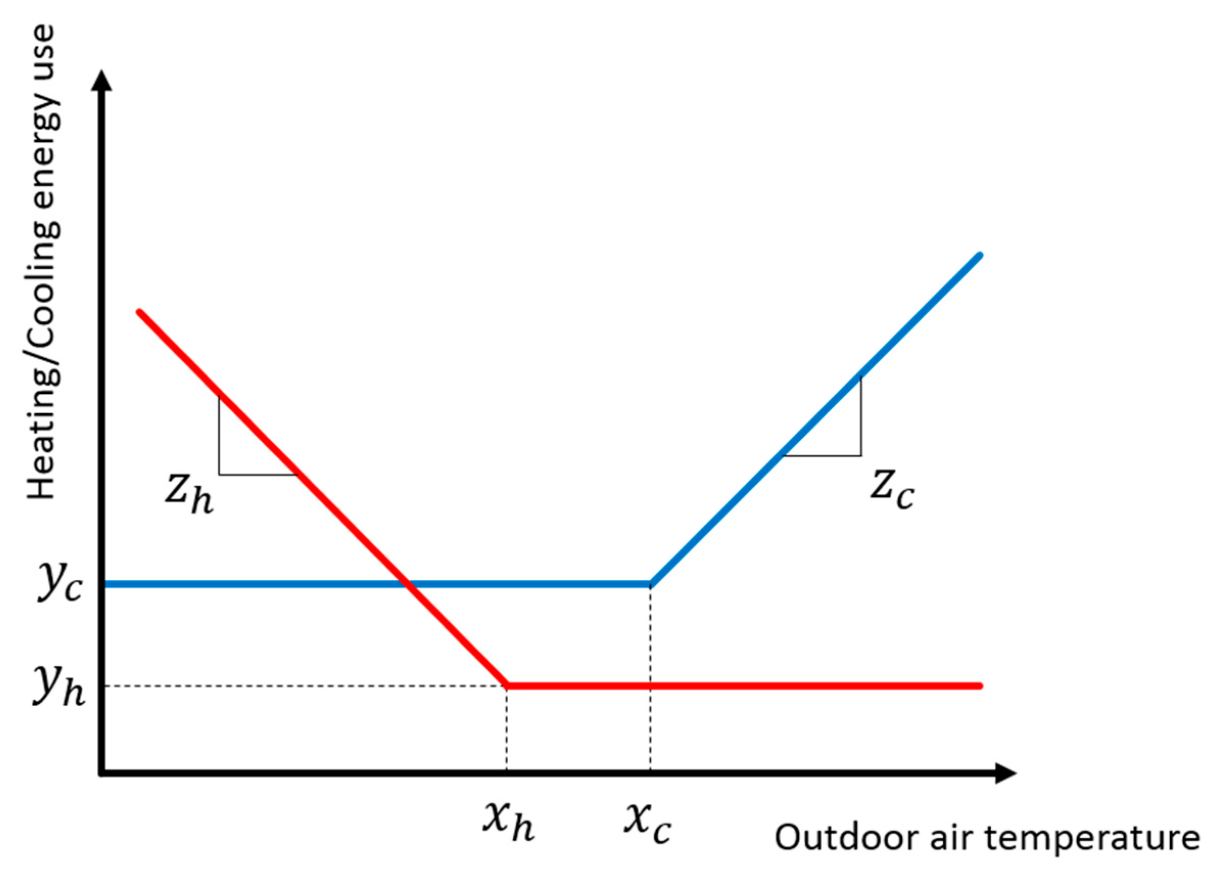
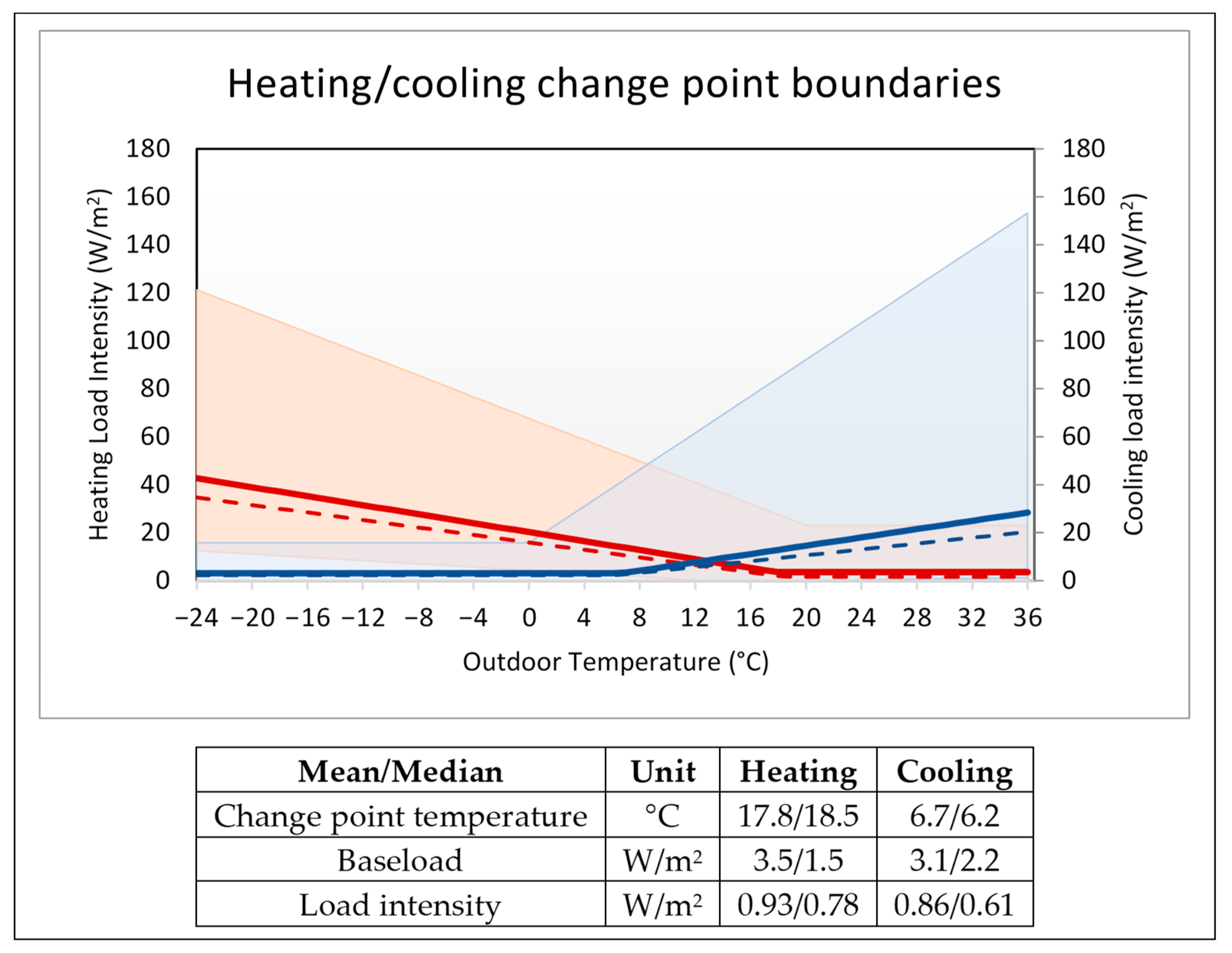
3.3. Thermal Load Change Point Analysis

Change point models, as proposed by ASHRAE in the early 2000s [32], provide a fit between heating or cooling energy use and outdoor air temperature. In this study, a modified change point model [33] is used as illustrated in Figure 3, and defined in a simple regression model in Equation (4) (heating) and Equation (5) (cooling).

$$Q_h=y_h+z_h\left(T_{out}-x_h\right)$$

(4)

$$Q_c=y_c+z_c\left(T_{out}-x_c\right)$$

(5)

Each of the heating and cooling change point models has three sets of parameters. Parameters x_h and x_c define the change point temperature for heating and cooling, respectively. This is the outdoor air temperature at which the building switches between providing only the base load (independent of outdoor temperature) and providing active heating/cooling based on the outdoor temperature. This temperature, also called the balance temperature, may also indicate the shift between off-season and on-season heating or cooling. In an ideal case, and to avoid simultaneous heating and cooling in a building, x_c should be higher than x_h. However, this condition is often violated in commercial buildings, resulting in a waste of energy. Parameters y_h and y_c indicate the y-intercept value and correspond to the base load for heating and cooling, respectively. This parameter is non-negative. In some buildings, the base loads are zero, meaning that there is no off-season heating or cooling. This is also a necessary condition to avoid simultaneous heating and cooling. However, in buildings with multiple zones that require strict following of zonal temperature setpoints (such as those with server rooms, laboratories, etc.) the base load is usually not zero. Finally, parameters z_h and z_c represent the slope of the line for the active part (for outdoor temperatures higher than the cooling change point or lower than the heating change point). This slope is a measure of heating/cooling intensity, which is how much additional energy is used for 1 degree Celsius of change in outdoor air temperature. For heating, the slope is a negative number, while for cooling it is a positive value. Note that heating and cooling loads compensate for additional heat loss through the building envelope. In other words, for two buildings of similar archetype that are located in the same climate zone, the one with a higher absolute slope has poorer envelope performance in terms of thermal insulation and/or air leakage. The parameters of the change point models are identified using a Genetic Algorithm optimization [33].

4. Results

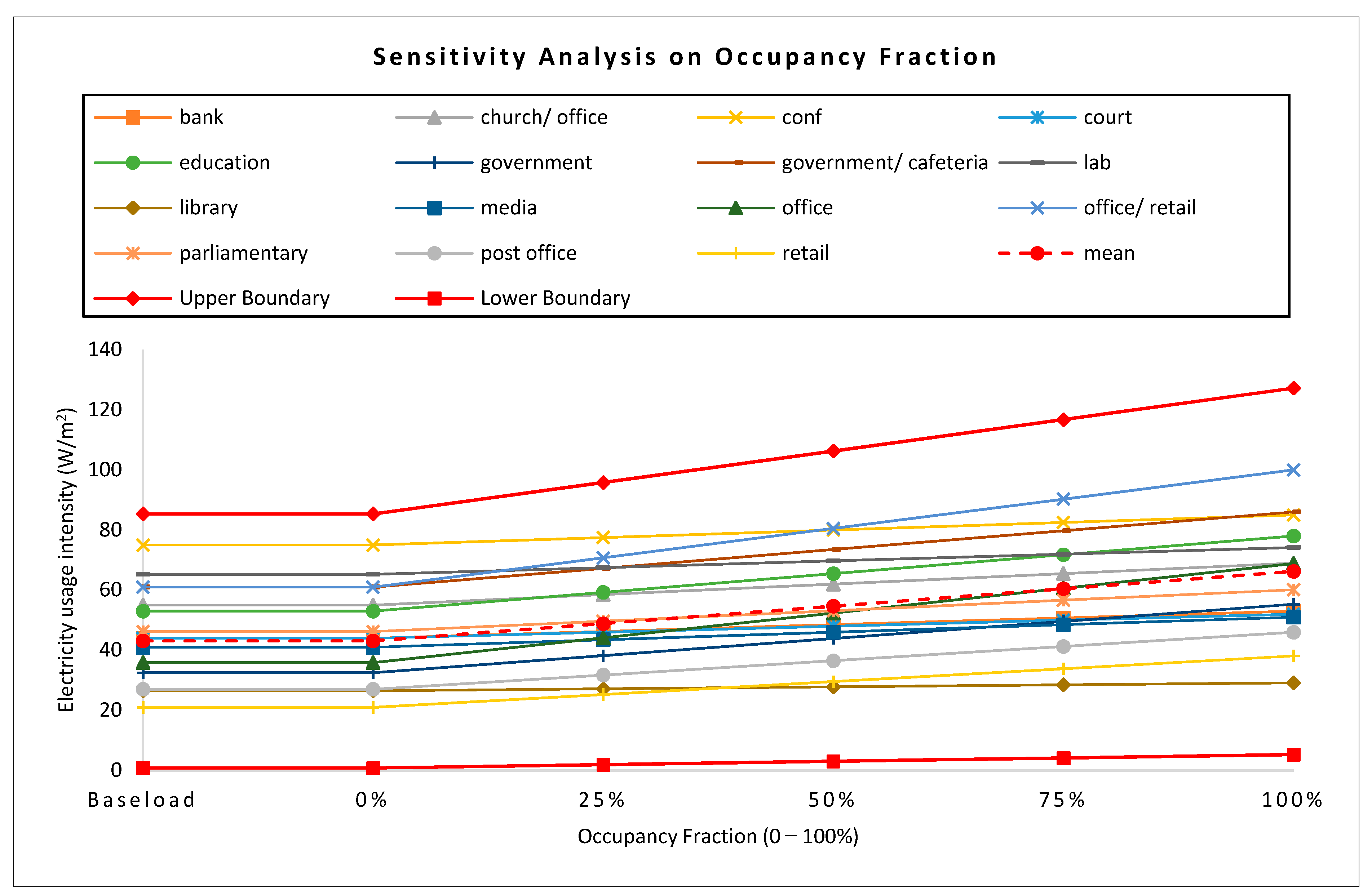
4.1. Electricity EUI Sensitivity to Occupancy (ESTO)

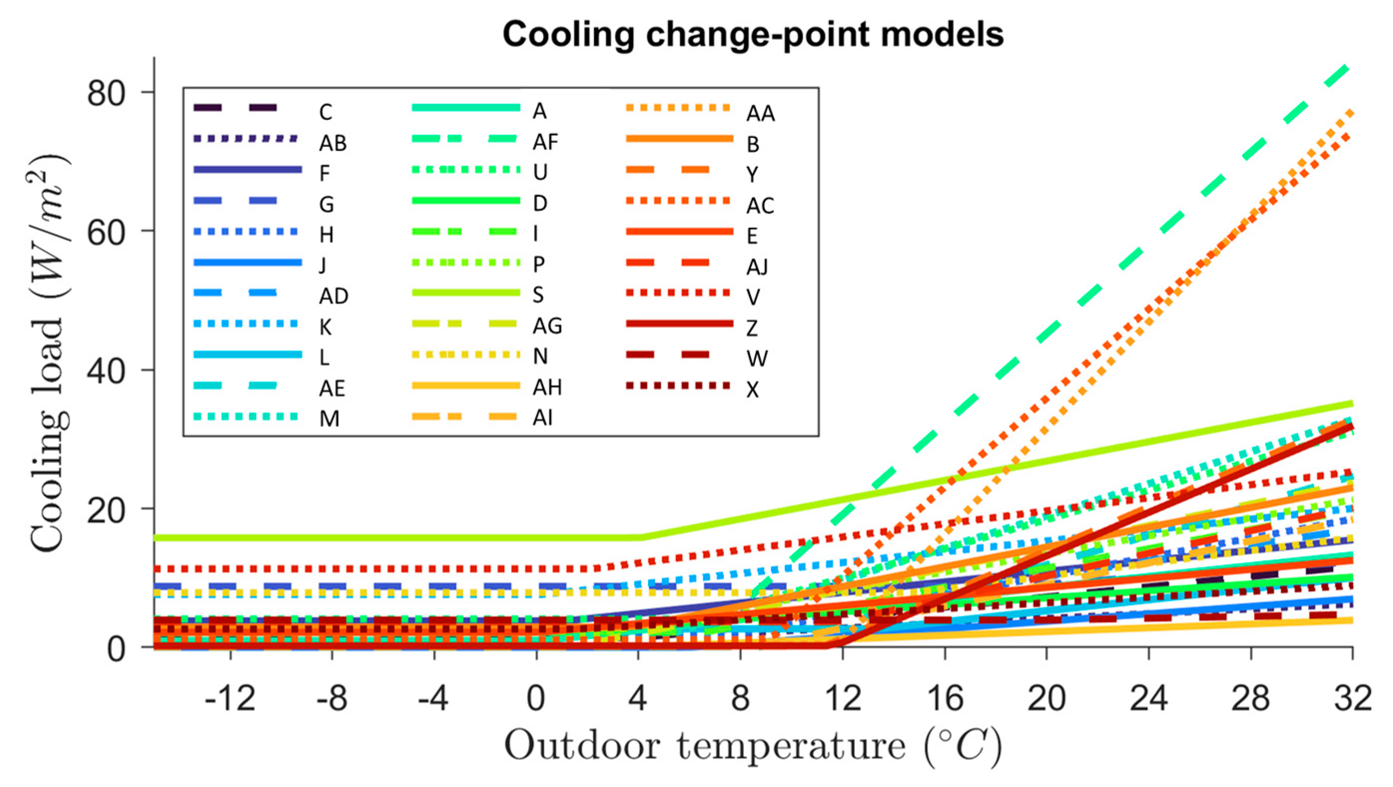
After validation [31], the ESTO model was deployed on all study buildings in which no objective occupancy data are available. It should be noted that the data set used in this current study is distinct from that used for demonstration in [31]. By knowing the base (night-time business-as-was-usual (i.e., night-time baseload pre-COVID), no-occupancy and typical full-occupancy electricity EUIs, and slope (calculated), we were able to establish a linear regression to estimate the electricity EUI for a given occupancy fraction. Figure 4 demonstrates the average per building archetype sensitivity of electricity EUI to occupancy. In other words, each line represents the average of a building archetype where the sampling size for each of the presented archetypes varies according to data availability. The mean value of all study buildings is plotted in dashed red, while the two solid red lines represent the lower and upper boundaries, calculated as “mean ± 2 standard deviations”. Values outside of the upper and lower boundary range are considered outliers. Here, the slope defines the impact of occupancy on electricity EUI on a scale between 0% (unoccupied) and 100% (typical business-as-usual occupancy). A steep slope indicates a high sensitivity to occupancy, or in other words, the more occupants, the higher electricity EUI. An obvious example is office buildings and educational facilities; where each typical occupant would turn on computing equipment and/or electronic devices. On the other hand, a flattened slope may indicate less sensitivity of the building’s electricity EUI to occupancy count, such as in the case of a library or church. The plot also shows and compares the average baseload per building archetype, where the lowest, median and highest are retail, court, and conference, respectively. A typical office building’s base load is 36 W/m², and laboratory is 65 W/m².

4.2. Cooling

Figure 5 shows change point models for cooling load. It can be seen that some of the models stand out by a higher intercept, a steeper line, or an early break point. In order to better investigate these anomalies, parameters of the change point models are listed in Table 2 for the studied buildings.

Figure 5. Change point models for cooling load. The decoding of the symbols, which denotes the investigated buildings, is given in Table 2.

Figure 5. Change point models for cooling load. The decoding of the symbols, which denotes the investigated buildings, is given in Table 2.

Table 2. Parameters of cooling change point models.

Name 1	Type	xc	yc	zc	Name	Type	xc	yc	zc	Name	Type	xc	yc	zc
A	Education	0	0.95	0.39	L	Post office	13.5	2.68	0.4	AA	Lab	11.8	0.43	3.82
B	Mixed	3.8	2.94	0.71	M	Parliamentary	4.6	1.16	1.16	AB	Office	3.6	1.32	0.17
C	Mixed	4	1.38	0.37	N	Parliamentary	14.8	7.88	0.46	AC	Lab	9.1	1.11	3.21
D	Library	0	2.12	0.25	P	Library	0.3	0.61	0.65	AD	Office	6.9	2.78	0.57
E	Bank	0.1	2.18	0.33	S	Media	4.1	15.78	0.69	AE	Government	9	0.1	1.07
F	Office	1.1	3.82	0.38	U	Mixed	6.4	4.09	1.05	AF	Lab	7.2	3.59	3.26
G	Parliamentary	18.9	8.79	0.27	V	Court	2.2	11.31	0.47	AG	Lab	1.4	0.07	0.77
H	Office	7.9	2.01	0.68	W	Parliamentary	20	3.95	0.07	AH	Office	5	0.24	0.14
I	Government	6.7	2.22	0.69	X	Parliamentary	1.7	2.65	0.21	AI	Office	8.6	0.13	0.78
J	Government	6	0.01	0.27	Y	Government	11.3	0.19	1.58	AJ	Office	11.9	3.69	0.81
K	Conf	0.3	7.65	0.39	Z	Office	11.7	0.23	1.56

¹ x_c—cooling balance temperature; y_c—cooling base load; z_c—cooling load intensity.

Table 2. Parameters of cooling change point models.

Name 1	Type	xc	yc	zc	Name	Type	xc	yc	zc	Name	Type	xc	yc	zc
A	Education	0	0.95	0.39	L	Post office	13.5	2.68	0.4	AA	Lab	11.8	0.43	3.82
B	Mixed	3.8	2.94	0.71	M	Parliamentary	4.6	1.16	1.16	AB	Office	3.6	1.32	0.17
C	Mixed	4	1.38	0.37	N	Parliamentary	14.8	7.88	0.46	AC	Lab	9.1	1.11	3.21
D	Library	0	2.12	0.25	P	Library	0.3	0.61	0.65	AD	Office	6.9	2.78	0.57
E	Bank	0.1	2.18	0.33	S	Media	4.1	15.78	0.69	AE	Government	9	0.1	1.07
F	Office	1.1	3.82	0.38	U	Mixed	6.4	4.09	1.05	AF	Lab	7.2	3.59	3.26
G	Parliamentary	18.9	8.79	0.27	V	Court	2.2	11.31	0.47	AG	Lab	1.4	0.07	0.77
H	Office	7.9	2.01	0.68	W	Parliamentary	20	3.95	0.07	AH	Office	5	0.24	0.14
I	Government	6.7	2.22	0.69	X	Parliamentary	1.7	2.65	0.21	AI	Office	8.6	0.13	0.78
J	Government	6	0.01	0.27	Y	Government	11.3	0.19	1.58	AJ	Office	11.9	3.69	0.81
K	Conf	0.3	7.65	0.39	Z	Office	11.7	0.23	1.56

¹ x_c—cooling balance temperature; y_c—cooling base load; z_c—cooling load intensity.

Variable x_c represents the cooling balance (or change point) temperature. The average balance temperature is 6.7 degrees Celsius and the standard deviation is 5.4. As a result, buildings with a balance temperature lower than −4.1 and higher than 17.5 are considered outliers. This includes buildings “G” and “W”.

Variable y_c represents the cooling base load. The average cooling base load is 3.1 Watts per square meter and the standard deviation is 3.6. As a result, buildings with a cooling base load higher than 10.3 are considered outliers. This includes buildings “S” and “V”. Variable z_c represents the cooling load intensity. The average cooling load intensity is 0.86 Watts per square meter and degree Celsius, and the standard deviation is 0.92. As a result, buildings with a cooling load intensity higher than 2.7 are considered outliers. This includes buildings “AA”, “AC”, and “AF”.

For cooling, overall, there is no single building with more than one type of abnormal change point parameter. Still, a couple of insights are found based on this analysis:

• Many buildings have a cooling balance temperature that is quite close to zero, meaning that the active cooling starts and ends in winter, rather than the shoulder seasons (keep in mind that we are using average daily temperatures). For this reason, the portfolio owner might want to check the criteria for starting up and shutting down the cooling system.
• As mentioned before, a necessary condition to avoid simultaneous heating and cooling is to have a base load equal to or close to zero. By inspecting Table 2, we see that only three buildings, “J”, “AE”, and “AG”, have a base load of 0.1 Watts per square meter or lower, hence the remaining buildings have some simultaneous heating and cooling that may need to be investigated.
• For “S” and “V” that have a high base load, the portfolio owner might want to check that there is no unwanted cooling in these buildings during the heating season.
• The load intensity is a good indication of envelope performance. As a result, for buildings “AF”, “Z”, and “AC”, envelope inspection (insulation, windows, ceiling, etc.) can be a priority point in the next audit schedule.

4.3. Heating

Similar to the cooling load, change point analyses are carried out for the heating load using the model shown in Figure 6.

Table 3. Parameters of heating change point models.

Name 1	Type	xh	yh	zh	Name	Type	xh	yh	zh	Name	Type	xh	yh	zh
A	Education	19.9	0.94	0.49	L	Post office	16.4	0.28	1.12	Z	Office	19.8	5.31	0.54
B	Mixed	16.8	3.05	0.76	M	Parliamentary	19.8	0.61	0.34	AA	Lab	17.8	6.01	1
C	Mixed	17.4	0.56	0.73	N	Parliamentary	15.4	0.02	0.78	AB	Office	18.5	1.26	0.92
D	Library	19.9	1.7	0.74	O	Retail	20	5.09	1.93	AC	Lab	16.4	14.28	2.18
E	Bank	16.1	2.47	0.83	P	Library	18.7	8.85	0.62	AD	Office	17.3	6.45	1.83
F	Office	19.8	0.44	0.59	R	Retail	19.3	0.37	2.23	AE	Government	12.5	0.17	0.78
G	Parliamentary	13.5	0.21	0.52	S	Media	19.9	1.81	0.65	AF	Lab	19.2	23.09	1.44
H	Office	19.6	3.5	0.64	U	Mixed	18.3	2.47	0.98	AG	Lab	16.8	0.57	1.12
I	Government	19.6	1.5	0.87	V	Court	19.8	4.13	1.45	AH	Office	16.2	0.2	0.48
J	Government	16.2	0.43	0.74	W	Parliamentary	19.4	0.59	0.45	AI	Office	15.6	0.31	0.54
K	Conf	19.6	12.67	0.82	Y	Government	20	0.89	0.61	AJ	Office	12.8	6.68	1.17

¹ x_c—heating balance temperature; y_c—heating base load; z_c—heating load intensity.

shows the heating change point parameters for the analyzed buildings.

Variable x_h represents the heating balance (or change point) temperature. The average balance temperature is 17.8 degrees Celsius and the standard deviation is 2.2. As a result, buildings with a balance temperature lower than 13.4 and higher than 22.2 are considered outliers. This includes buildings “AE” and “AJ”. Variable y_h represents the heating base load. The average heating base load is 3.5 Watts per square meter and the standard deviation is 5. As a result, buildings with a heating base load higher than 13.6 are considered outliers. This includes buildings “AC” and “AF”. Variable z_h represents the heating load intensity. The average heating load intensity is 0.94 Watts per square meter and degrees Celsius, and the standard deviation is 0.5. As a result, buildings with a heating load intensity higher than 1.93 are considered outliers. This includes buildings “O”, “R”, and “AC”.

For heating, overall, the only building with two abnormal change point parameters is “AC”, where there seems to be a high potential to lower steam usage. Similarly, the following insights are extracted from the analysis:

• In terms of heating balance temperature, the highest value observed is 20 degrees Celsius. For Ottawa, this average daily temperature is usually crossed in the months of May and September, meaning that the heating system is properly started and stopped in the shoulder seasons. For “AE” and “AJ” that have a low heating balance temperature, this might create a comfort problem for the occupants by delaying the start of the active heating season to a later time.
• Regarding the base load, similar arguments to the one made for cooling can be made. Only one building, “N”, has a base load close to zero. This means that almost all buildings are prone to experience simultaneous heating and cooling and waste energy, particularly for buildings “AC” and “AF”.

In terms of heating load intensity, outlier buildings, “O”, “R”, and “AC” are candidates for the investigation of air leakage and insufficient insulation.

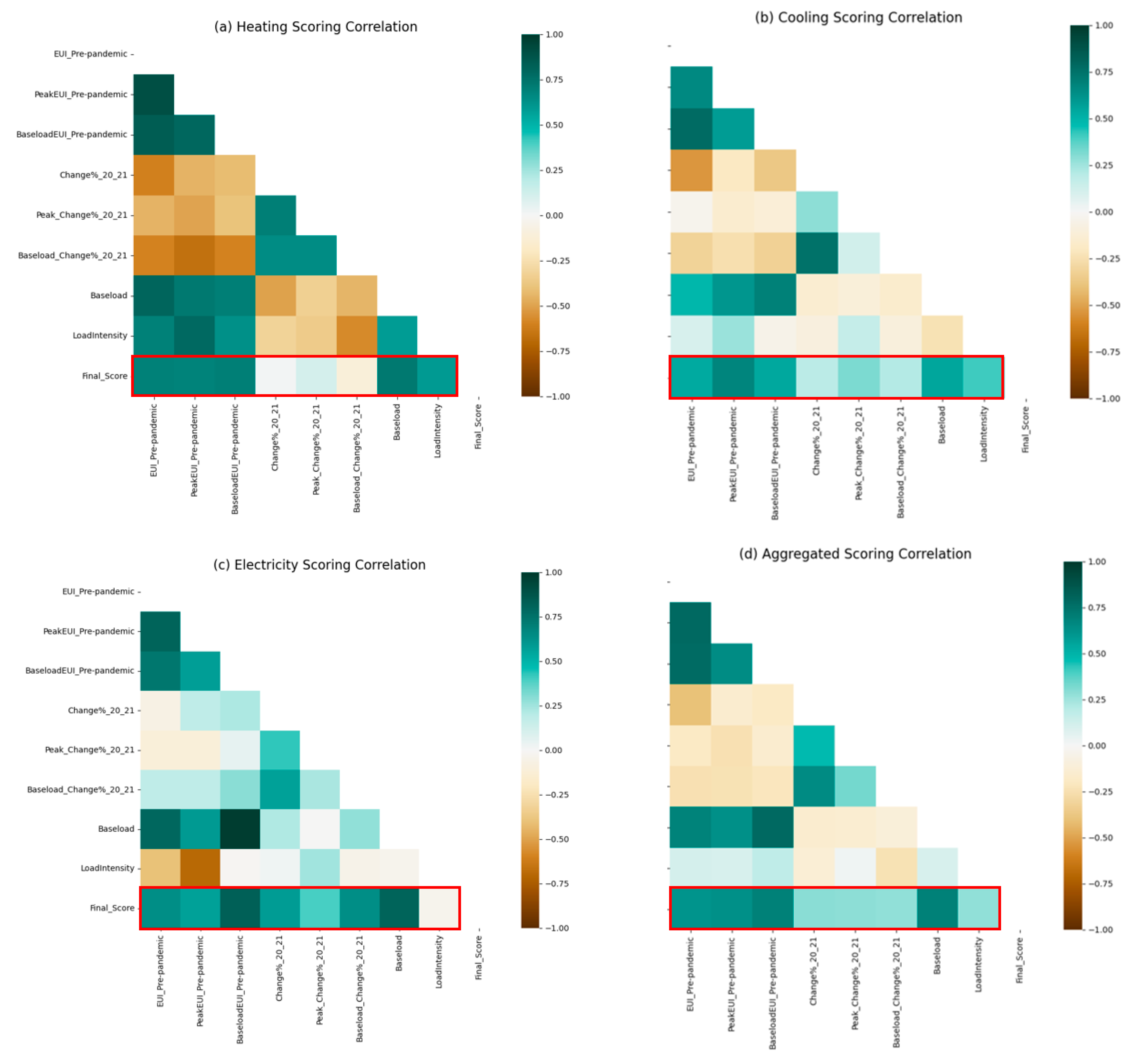
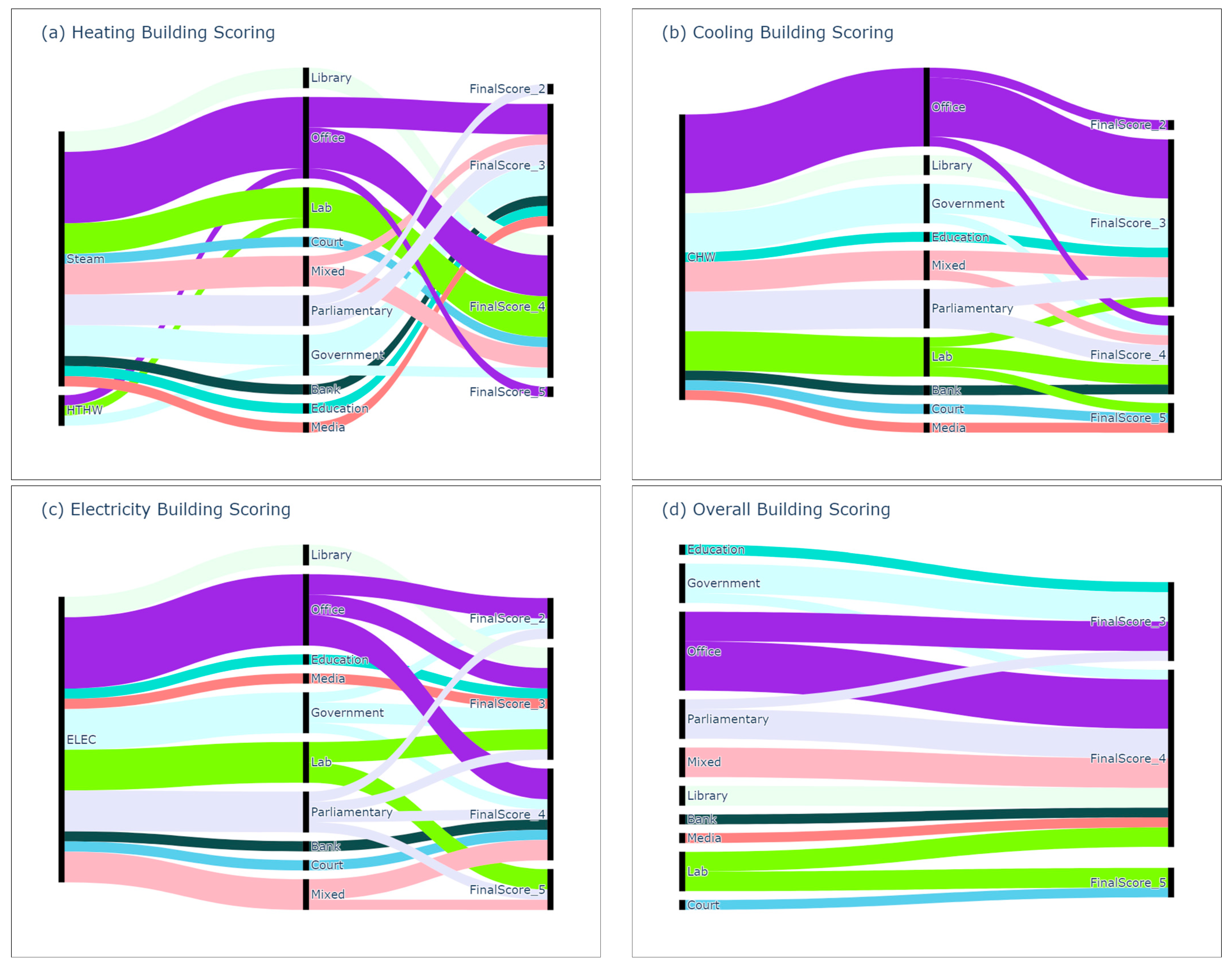
5. Performance Scorecard

In an effort to mitigate the worst impacts of climate change, the Government of Canada proposed the goal of achieving net-zero emissions by 2050 [34]. To reduce the carbon footprint from the building sector, it is necessary to reduce the energy consumption and greenhouse gas emissions from the existing building stock. The most effective impact can be obtained by targeting and prioritizing retrofits for the poorest performing buildings within a given portfolio. In this section, we aim to develop a systematic method to assess building performance based on multiple parameters, then provide a scorecard (i.e., ranking) within a building’s own portfolio. In order to collectively assess the energy performance of buildings, especially in cases where multiple energy sources are used, the most effective criteria first need to be identified. In

Table 4. Selected parameters for building energy performance scorecard calculation.

	Energy Type/Parameter	Electricity	Cooling	Heating	Ranking Order (Ap,b) 1
Baseline/Pre-pandemic	Annual EUI	Y	Y	Y	Ascending 2
	Peak EUI	Y	Y	Y
	Baseload (year-round) EUI	Y	Y	Y
Deviation in FY20_21%	Annual	Y	Y	Y
	Peak	Y	Y	Y
	Baseload (year-round)	Y	Y	Y
Change Point model	Baseload (off-season)	-	Y	Y
	Load intensity	-	Y	Y
ESTO model	Baseload	Y	-	-
	Load intensity	Y	-	-	Descending

¹ 1 is most efficient and n_id (for n_id is the dimension of the vector space) is least efficient). ² Lowest annual EUI ranks as most efficient and so on throughout the Table.

, a summary of the selected performance parameters is presented. In this study, we summarized the annual aggregated EUI per building archetype in Figure 2. Peak and baseload values for a similar (but not identical) dataset can be found in [10]. Additionally, results from the change point model (for heating and cooling) and ESTO model (for electricity) are used to assess the building energy efficiency. For all parameters (except for ESTO load intensity), we assume that the lower the usage intensity the better the building performance, given that all values are normalized per floor area and, moreover, all heating and cooling values are weather normalized for comparability. For ESTO load intensity, we assume that buildings with low sensitivity to occupancy may either lack zoning or, simply, over-consume electricity during low occupancy. On a weekday, a typical office building would have an average baseload/peak load split of 15/100 and 40/100 for lighting and plug loads, respectively; or approximately 30/100, collectively [35]. In the case of the study buildings in this study, we find an average baseload/peak load split of 60/100. In future studies, a deeper investigation of baseload/peak load breakdown components should be carried out.

Rank ordering (A_e,p,id) where A denotes the rank (between 1 and n_id where n_id is the dimension of the vector space or, in other words, number of study buildings), e denotes the energy type, p denotes the performance parameter, and id denotes the unique building id, was carried out for each parameter independently, where the lowest order for each parameter represents the best performing building (the opposite is true for ESTO load intensity). It should be noted that the ranking is based on a comparison between this specific set of buildings; hence, eliminating parts of, or extending, this set of data may incur a change in the ranking order. An integer score from 1 to 5 was assigned to each individual performance parameter for each unique building based on the ranking order, where 1 is the best performing, as follows in Equation (6):

$$Score{ }_{e,p,id}= \lceil \frac{A{ }_{e,p,id}}{n_{id}}\times 5\rceil$$

(6)

Finally, the final score Score_f,id for each individual building is calculated based on the ceiling of the equally weighted average score out of the eight selected performance parameters n_p for all energy types n_e collectively (represented in Equation (7) as n_p or number of performance parameters) in Table 4.

$$Score{ }_{f,id}= \lceil {{\displaystyle \sum }}_1^{n_p}\frac{{{\displaystyle \sum }}_1^{n_e}\frac{Score{ }_{p,id}}{n_e}}{n_p}\rceil$$

(7)

The final score for each building, summarized in

Table 5. Summary of building performance scores at the building, energy type, and performance parameter levels. “T” in last column represents the total final score.

Performance Param.		EUI_Pre-Pandemic			Peak EUI Pre-Pandemic			Baseload EUI Pre-Pandemic			Change % 20_21			Peak_Change % 20_21			Baseload_Change % 20_21			Baseload			Load Intensity			Final Score
Energy Type 1		C	E	H	C	E	H	C	E	H	C	E	H	C	E	H	C	E	H	C	E	H	C	E	H	C	E	H	T
A	Education	4	4	4	3	4	4	5	4	4	1	1	1	1	1	1	1	1	1	2	4	3	2	2	1	3	3	3	3
B	Mixed	4	4	2	4	4	2	4	4	3	1	3	5	2	1	4	1	3	4	4	4	4	4	4	3	3	4	4	4
C	Mixed	1	5	2	1	5	2	2	5	3	5	5	4	5	2	4	4	5	2	3	5	2	2	1	2	3	5	3	4
D	Library	3	1	3	2	1	3	4	3	4	2	5	5	2	5	5	2	1	4	3	3	3	1	5	3	3	3	4	4
E	Bank	3	4	4	3	3	4	3	4	2	3	2	1	5	4	1	4	4	1	3	4	4	2	5	4	4	4	3	4
F	Office	4	3	2	5	3	3	3	4	3	3	4	4	1	2	2	4	4	4	4	4	2	2	2	2	4	4	3	4
G	Parliamentary	4	1	2	4	1	1	5	3	2	2	2	4	3	4	5	2	3	5	5	2	1	1	5	1	4	3	3	4
H	Office	2	2	3	2	3	3	3	2	4	2	5	3	1	4	2	1	5	4	3	2	4	3	2	2	3	4	4	4
I	Government	3	4	2	3	5	3	3	3	1	4	5	5	2	3	4	4	5	5	3	3	3	3	1	4	4	4	4	4
J	Government	1	2	2	1	2	2	1	3	3	5	3	3	2	1	2	5	3	3	1	3	2	1	4	3	3	3	3	3
M	Parliamentary	4	1	1	3	1	1	4	2	1	1	2	2	2	2	2	2	2	3	2	2	2	5	4	1	3	2	2	3
N	Parliamentary	2	3	2	5	5	2	3	5	2	5	5	3	1	5	1	5	5	4	5	4	1	3	2	3	4	5	3	4
P	Library	3	1	3	2	1	3	2	1	4	4	5	4	3	5	4	4	5	4	2	1	5	3	5	2	3	3	4	4
S	Media	4	4	1	4	3	1	5	3	2	5	1	2	5	2	3	5	2	3	5	3	3	3	4	2	5	3	3	4
U	Mixed	5	5	4	5	4	3	5	5	5	1	2	2	1	3	2	1	4	2	5	5	4	4	2	4	4	4	4	4
V	Court	5	3	5	5	2	4	5	4	5	4	3	2	4	3	3	2	2	2	5	4	4	3	5	5	5	4	4	5
X	Parliamentary	3	4		2	3		4	4		4	3		4	3		3	3		3	4		1	4		3	4		4
Y	Government	2	1	3	2	2	2	2	2	2	4	4	2	2	2	5	5	4	5	1	2	3	5	3	2	3	3	3	3
Z	Office	1		3	1		2	1		2	5		4	5		5	5		5	1		4	5		1	3		4	4
AA	Lab	5	2	5	4	1	5	3	3	5	2	2	1	3	5	2	3	3	1	2	3	5	5	5	4	4	3	4	4
AB	Office	5	3	3	3	4	4	2	2	3	1	1	5	4	1	3	2	1	2	3	2	3	1	1	4	3	2	4	3
AC	Lab	5	5	5	5	5	5	4	5	5	3	4	1	4	5	1	3	2	1	2	5	5	5	3	5	4	5	4	5
AD	Office	2	3	5	3	3	5	3	1	5	3	2	2	3	5	3	3	2	3	4	1	5	3	1	5	3	3	5	4
AE	Government	2	2	1	2	2	2	1	1	2	2	1	4	4	3	5	3	1	2	1	1	1	5	2	3	3	2	3	3
AF	Lab	5	5	5	5	5	5	5	5	5	3	4	1	4	4	1	3	4	1	4	5	5	5	3	5	5	5	4	5
AG	Lab	1	3	3	5	4	4	1	2	4	5	3	5	3	3	4	2	2	3	1	2	2	4	2	4	3	3	4	4
AH	Office	1	1	1	1	2	1	1	1	1	4	3	4	1	3	4	5	3	5	2	1	1	1	3	1	2	3	3	3
AI	Office	1	3	1	1	4	1	1	2	1	3	1	5	5	1	5	1	1	5	1	2	1	4	1	1	3	2	3	3
AJ	Office	2	5	4	4	5	4	2	5	4	2	3	2	3	4	3	1	4	2	4	5	5	4	1	5	3	4	4	4

¹ C—cooling; H—heating; E—electricity; T—total score including all energy types.

, is used to order the building within its corresponding building portfolio ascendingly from best performing (i.e., 1) to worst performing (i.e., 5). The highest possible final score of a building (for example, 5) means that this building had multiple poor performing parameters for one or more energy types, prioritizing it for further investigation, or nominating it as a candidate for retrofit. Pearson correlation coefficient analysis amongst all the scores of each selected parameter was calculated as summarized in Figure 7, where a breakdown of (a) heating, (b) cooling, and (c) electricity is presented in Figure 7a–c, and aggregated (all energy types combined) is presented in Figure 7d. The parameter of interest in the correlation analysis is the “final score”. Here, a correlation coefficient indicates the impact of the score of each performance parameter on the final score of a building. Baseload appears to have had the strongest correlation and largest contribution to the final score, especially for heating, electricity, and aggregated energy. This means that there is a strong tie between a building’s poor performance and its high baseloads (i.e., afterhours electricity loads and off-season heating/cooling loads). For cooling energy, cooling peak load intensity appears to be the strongest contributor to the building’s final score, followed by baseload.

High cooling load intensity is associated with high steam (heating) base loads. This may indicate simultaneous heating and cooling, especially during shoulder seasons. Figure 8 presents a Sankey diagram demonstrating a breakdown of building final scores by energy type (heating, cooling, electricity, and aggregated energy), building archetype, and score, whereas the flow thickness indicates the building count. The aggregated energy score (Figure 8d) shows the average score of all three energy types, rounded up to the next highest integer. Office buildings have consistently better performance for all energy types, as compared to the other building archetypes presented in this study, especially for cooling. On the other hand, laboratories indicate a relatively poor scoring for cooling and electricity, and an average performance for heating. Mixed-use buildings (e.g., office building/retail, government/food service, office/church) are found to have had the poorest scoring for electricity usage but average scoring for both heating and cooling. Building archetypes with most variability in scoring are office buildings, laboratories, and parliamentary. The variability can be caused by user’s behavior, but also can be due to the relatively larger data sample size.

6. Discussion

6.1. ESTO

The methodology discussed in Section 3.1 allows the use of relative occupancy (i.e., hybrid work environment, shutdowns, over-occupancy) as a proxy to predict and keep track of electrical demand. As summarized in Figure 4, it is clear that base load varies widely across the different building archetypes, depending on their lighting, plug loads, and HVAC requirements. For example, office buildings with large server rooms can be highly load intensive compared to typical office buildings. Retail may have fairly low base loads outside of the hours of operation, but substantially higher loads prior to and during service hours. However, certain outliers may require the building operator’s attention, such as (1) buildings with base loads exceeding the statistically acceptable boundary range (i.e., mean ± 2 standard deviations), such as base loads above 85 W/m², and (2) also, flat horizontal lines in Figure 4 indicating a lack of sensitivity to occupancy, and therefore a lack of occupant-centric controls, especially for lighting and HVAC electric loads [36].

For the study buildings, since no information on the actual number of occupants was available (we only assumed fractions based on typical pre-pandemic occupancy), there could be multiple explanations for the slope-defining electricity usage intensity: (1) typical occupancy could be normally quite low and have less of an effect on plug loads (e.g., maintenance buildings could be electric load intensive and hence, electric loads are less sensitive to occupant behavior); (2) lack of occupant-centric controls for lighting, plug loads, and ventilation components may result in a full operation regardless of the number of occupants; (3) some buildings may have been fully or partially operated remotely (e.g., laboratories or office buildings with large server rooms). This may explain why only about a 5% reduction during the first year following the COVID-19 pandemic lockdown order was observed.

The novelty of this method as opposed to previous studies on the impact of occupancy and occupant behavior on energy use [4,36] is that this model does not require ground truth occupancy data, merely a record of energy use pre- and post- a pandemic lockdown order (or any other event incurring a sustained, and unplanned unoccupied period with normal energy service). Therefore, it can be widely applicable to the commercial buildings sector at large. On the other hand, it should be noted that this method may be associated with a larger margin of error.

6.2. Change Point Model

A change point analysis was carried out for heating and cooling loads. Three model parameters were identified using a genetic algorithm optimization in order to identify buildings with high load intensities, abnormal balance temperatures, or high base loads. The analysis concluded that some buildings are showing signs of simultaneous heating and cooling, and others potentially have a low performing envelope. The results can be used to rank buildings in terms of scheduling and envelope performance to identify the most critical buildings.

Table 2 and Table 3 can both be used to rank the buildings based on envelope performance. Additionally, by comparing the slope, change point temperature, and off-season base loads for both heating and cooling loads, insights about the building envelope can be extracted. For example, high cooling loads and low heating loads may indicate a high heat gain coefficient. Conversely, a low cooling load and high heating load may indicate a high infiltration rate. Figure 9 summarizes the heating and cooling change point model fits in terms of mean, median, maximum, and minimum values of each parameter considering all study buildings. The maximum ranges are based on the maximum value of each parameter combined (e.g., maximum base load, load intensity, and change point temperature (minimum for cooling change point temperature) combined). The maximum and minimum ranges may not represent an existing case of a building, but rather the highest/lowest possible scenarios based on the feed-in information from the studied buildings. The mean heating change point temperature is 17.8 °C, which is consistent with expectations. However, the mean cooling change point is 6.7 °C, which is relatively low, and might be tied to high internal/external heat gains. The baseload for heating and cooling are quite comparable at 3.5 W/m² and 3.1 W/m², respectively. In a heating-driven location such as the case of Ottawa, Canada, it is expected that buildings experience higher heating load intensity than the cooling counterpart, especially due to strong winds and relatively high humidity. This can be clearly interpreted through the load intensity (slope) values summarized in Figure 9. For example, a heating load intensity of 0.93 means that with each 1 °C drop in outdoor temperature, an additional 0.93 W/m² is needed to keep the indoor temperature of the building at its temperature set point.

6.3. Summary of Discussion

Findings from this study suggest that there is a potential for energy savings by reducing energy wasted during unoccupied periods (such as non-operating hours, weekends and holidays, and longer-term shutdowns), especially for occupant driven loads (such as plug loads and ventilation). Hence, this finding also applies for variable occupancy scenarios resulting from hybrid and flexible work schedules. Occupant-centric control (also referred to as demand-controlled operation) is one recommended practical solution that can support the adaptive behavior of buildings. Zoning, hoteling, and smart power strips can also reduce unoccupied building energy waste.

For thermal loads, the three-point change point model was deployed to determine the heating/cooling baseload, change point temperature, and load intensity for each of the study buildings. Buildings with lower baseload and/or load intensity indicate higher envelope efficiency given that the temperature set point is set to a reasonable indoor air quality and that human comfort is not compromised. Thus, moving forward, buildings that had relatively high baseload and/or load intensity can be identified and further investigated for their building envelope efficiency. At this point, preliminary assumptions for deficiencies such as high external heat gains, thermal bridging, high window-to-wall ratio, as well as mechanical system faults such as simultaneous heating and cooling may be made. However, further investigation may be required to validate such preliminary assumptions.

7. Conclusions and Future Work

This research aimed to (1) evaluate the post-pandemic energy performance of commercial buildings given the uncertainties pertaining to partial occupancy scenarios, novel ventilation mandates, and lack of occupancy-based controls; (2) propose a framework to assess both weather-driven (heating and cooling) and occupant-driven (electricity: lighting, plug loads, ventilation) energy performance; and (3) propose a scorecard methodology to rank buildings within a given portfolio from best to worst performing according to a set of performance criteria.

It should be noted that, like many government and commercial buildings, objective occupancy count data were not available. Instead, in order to understand the relationship between occupancy-driven energy usage and occupant behavior, we proposed a novel method to account for electricity sensitivity to occupancy (ESTO). The ESTO model was developed using “nearly” black box methods, shedding light on the impacts of occupancy on electricity usage intensity and allowing stakeholders to estimate future partial occupancy scenarios, while using very limited information. It also facilitates the identification of buildings that may need smart sensor retrofits for improved zoning moving forward. For example, motion sensors for lighting, demand-controlled ventilation, etc. The strength of the proposed method is that it is widely applicable and repeatable given easily accessible information. In this study, we took advantage of the COVID-19 pandemic lockdown period to measure electricity usage during periods when buildings are clearly unoccupied and compared it with typical full occupancy loads while subtracting baseloads from both scenarios. An alternative could be a holiday occurring on a weekday (non-weekend) when buildings are unoccupied but are also scheduled for normal weekday operation. Future studies should focus on day-ahead prediction of occupancy fraction in commercial buildings.

The three-point change point model was utilized to assess the thermal load performance of the building portfolio during the COVID-19 pandemic lockdown period, identifying three key parameters: baseload, heating/cooling load intensity, and the outdoor air temperature at which active heating/cooling starts. Compared to their own portfolio, buildings with poor performance in one or more of the key parameters can be identified for further investigation. High thermal load intensity may indicate either building envelope deficiencies (e.g., infiltration, thermal bridging, poor insulation, heat gains), or faulty HVAC operation (e.g., hard or soft faults). High off-season baseloads may indicate simultaneous heating and cooling or lack of proper scheduling. Change point temperature may be intuitive of indoor comfort levels.

The proposed performance scorecard is based on ranking the buildings within a given building portfolio from best to worst performing according to eight selected performance criteria for each energy type, where these performance criteria are equally weighted. The ranking of each building is then adjusted to a score between 1 and 5, where 1 represents best performance. One interesting finding is that baseload had the most significant influence on building scoring. In other words, buildings with relatively high baseload intensities (for one or more energy type) are most likely to have the poorest performance. For cooling loads, peak load intensity also indicated strong influence on the building score. Future work should include the following:

• Application of time-series decomposition methods to filter out noise, seasonality and residuals, and only compare the highest and lowest points on the trend [27]. It is critical to isolate weather and other possible parameters that may affect the electricity usage trends.
• It is critical to disaggregate electrical loads to user-dependent (e.g., kitchen appliances, personal devices, lighting intensity) and user-independent (e.g., security systems, lab equipment, servers, baseloads for minimum HVAC operation, especially in winter months) in order to fully capture the effects of occupancy on electricity usage intensity. The method we proposed was able to capture user-independent baseloads during the COVID-19 pandemic ad hoc lockdown period. In the future, we aim to cross validate those findings by conducting either field visits, questionnaires, or, if possible, submetering for major plug loads.
• Cross-validate the proposed method with occupancy data from one or more study buildings. Proxies for occupancy such as security access badge-in (combined with badge-out), Wi-Fi information, or CO2 concentration have proven to be useful at varying degrees of accuracy.
• Expand the model to include all-season data, not only shoulder season data.

At the time of writing, the world is in the recovery stage of the COVID-19 pandemic, where reduced building capacity is taken into consideration as one of the preventative measures to reduce airborne transmission of diseases. That said, hybrid and partial occupancy in commercial and government office buildings has become the “new normal”. Pre-pandemic typical business-as-usual occupancy schedules are about to become business-as-was-usual. The most challenging roadblocks from a building energy management viewpoint are: (1) operating the building in the most energy-efficient manner during partial occupancy; (2) while doing so, maintaining healthy indoor air quality (i.e., improving ventilation) and comfort settings; and (3) predicting occupancy ahead of time in order to make energy- and carbon-wise decisions. Future work should investigate zoning options for large multi-story office buildings, the feasibility of occupant-centric controls, improved air quality sensors, and methods to quantify the adaptability of existing buildings to such suggested solutions.

References

1. International Energy Agency. Covid-19 Impact on Electricity; IEA: Paris, France, 2020. [Google Scholar]
2. Soava, G.; Mehedintu, A.; Sterpu, M.; Grecu, E. The Impact of the COVID-19 Pandemic on Electricity Consumption and Economic Growth in Romania. Energies 2021, 14, 2394. [Google Scholar] [CrossRef]
3. United Nations. WHO Chief Declares End to COVID-19 as a Global Health Emergency. Available online: https://news.un.org/en/story/2023/05/1136367 (accessed on 18 August 2023).
4. Gunay, H.B.; Ouf, M.; Newsham, G.; O’Brien, W. Sensitivity Analysis and Optimization of Building Operations. Energy Build. 2019, 199, 164–175. [Google Scholar] [CrossRef]
5. Beyer, R.C.M.; Franco-Bedoya, S.; Galdo, V. Examining the Economic Impact of COVID-19 in India through Daily Electricity Consumption and Nighttime Light Intensity. World Dev. 2021, 140, 105287. [Google Scholar] [CrossRef] [PubMed]
6. Santiago, I.; Moreno-Munoz, A.; Quintero-Jiménez, P.; Garcia-Torres, F.; Gonzalez-Redondo, M.J. Electricity Demand during Pandemic Times: The Case of the COVID-19 in Spain. Energy Policy 2021, 148, 111964. [Google Scholar] [CrossRef] [PubMed]
7. Ding, Y.; Ivanko, D.; Cao, G.; Brattebø, H.; Nord, N. Analysis of Electricity Use and Economic Impacts for Buildings with Electric Heating under Lockdown Conditions: Examples for Educational Buildings and Residential Buildings in Norway. Sustain. Cities Soc. 2021, 74, 103253. [Google Scholar] [CrossRef]
8. Henderson, J.V.; Squires, T.; Storeygard, A.; Weil, D. The global distribution of economic activity: Nature, history, and the role of trade. Q. J. Econ. 2017, 133, 357–406. [Google Scholar] [CrossRef] [PubMed]
9. Buechler, E.; Powell, S.; Sun, T.; Astier, N.; Zanocco, C.; Bolorinos, J.; Flora, J.; Boudet, H.; Rajagopal, R. Global Changes in Electricity Consumption during COVID-19. iScience 2022, 25, 103568. [Google Scholar] [CrossRef] [PubMed]
10. Awad, H.; Ashouri, A.; Bahiraei, F. Implications of COVID-19 for Electricity Use in Commercial Smart Buildings in Canada—A Case Study. In Proceedings of the eSim 2022: 12th Conference of IBPSA, Ottawa, ON, Canada, 22–23 June 2022; International Building Performance Simulation Association (IBPSA): Ottawa, ON, Canada, 2022. [Google Scholar]
11. Leach, A.; Rivers, N.; Shaffer, B. Canadian Electricity Markets during the COVID-19 Pandemic: An Initial Assessment. Can. Public Policy 2020, 46, S145–S159. [Google Scholar] [CrossRef]
12. Burleyson, C.D.; Rahman, A.; Rice, J.S.; Smith, A.D.; Voisin, N. Multiscale Effects Masked the Impact of the COVID-19 Pandemic on Electricity Demand in the United States. Appl. Energy 2021, 304, 117711. [Google Scholar] [CrossRef]
13. Zhang, X.; Pellegrino, F.; Shen, J.; Copertaro, B.; Huang, P.; Kumar Saini, P.; Lovati, M. A Preliminary Simulation Study about the Impact of COVID-19 Crisis on Energy Demand of a Building Mix at a District in Sweden. Appl. Energy 2020, 280, 115954. [Google Scholar] [CrossRef]
14. Rouleau, J.; Gosselin, L. Impacts of the COVID-19 Lockdown on Energy Consumption in a Canadian Social Housing Building. Appl. Energy 2021, 287, 116565. [Google Scholar] [CrossRef] [PubMed]
15. Li, L.; Meinrenken, C.J.; Modi, V.; Culligan, P.J. Impacts of COVID-19 Related Stay-at-Home Restrictions on Residential Electricity Use and Implications for Future Grid Stability. Energy Build. 2021, 251, 111330. [Google Scholar] [CrossRef] [PubMed]
16. Halbrügge, S.; Schott, P.; Weibelzahl, M.; Buhl, H.U.; Fridgen, G.; Schöpf, M. How Did the German and Other European Electricity Systems React to the COVID-19 Pandemic? Appl. Energy 2021, 285, 116370. [Google Scholar] [CrossRef] [PubMed]
17. Bahmanyar, A.; Estebsari, A.; Ernst, D. The Impact of Different COVID-19 Containment Measures on Electricity Consumption in Europe. Energy Res. Soc. Sci. 2020, 68, 101683. [Google Scholar] [CrossRef] [PubMed]
18. Delgado, D.B.d.M.; de Lima, K.M.; Cancela, M.d.C.; Siqueira, C.A.d.S.; Carvalho, M.; de Souza, D.L.B. Trend Analyses of Electricity Load Changes in Brazil Due to COVID-19 Shutdowns. Electr. Power Syst. Res. 2021, 193, 107009. [Google Scholar] [CrossRef]
19. Norouzi, N.; Zarazua de Rubens, G.; Choubanpishehzafar, S.; Enevoldsen, P. When Pandemics Impact Economies and Climate Change: Exploring the Impacts of COVID-19 on Oil and Electricity Demand in China. Energy Res. Soc. Sci. 2020, 68, 101654. [Google Scholar] [CrossRef] [PubMed]
20. Kirli, D.; Parzen, M.; Kiprakis, A. Impact of the Covid-19 Lockdown on the Electricity System of Great Britain: A Study on Energy Demand, Generation, Pricing and Grid Stability. Energies 2021, 14, 635. [Google Scholar] [CrossRef]
21. Alhajeri, H.M.; Almutairi, A.; Alenezi, A.; Alshammari, F. Energy Demand in the State of Kuwait During the Covid-19 Pandemic: Technical, Economic, and Environmental Perspectives. Energies 2020, 13, 4370. [Google Scholar] [CrossRef]
22. Malec, M.; Kinelski, G.; Czarnecka, M. The Impact of Covid-19 on Electricity Demand Profiles: A Case Study of Selected Business Clients in Poland. Energies 2021, 14, 5332. [Google Scholar] [CrossRef]
23. Agdas, D.; Barooah, P. Impact of the COVID-19 Pandemic on the U.S. Electricity Demand and Supply: An Early View from Data. IEEE Access 2020, 8, 151523–151534. [Google Scholar] [CrossRef]
24. Abu-Rayash, A.; Dincer, I. Analysis of the Electricity Demand Trends amidst the COVID-19 Coronavirus Pandemic. Energy Res. Soc. Sci. 2020, 68, 101682. [Google Scholar] [CrossRef]
25. Santiago, I.; Lopez-Rodriguez, M.A.; Trillo-Montero, D.; Torriti, J.; Moreno-Munoz, A. Activities Related with Electricity Consumption in the Spanish Residential Sector: Variations between Days of the Week, Autonomous Communities and Size of Towns. Energy Build. 2014, 79, 84–97. [Google Scholar] [CrossRef]
26. López Prol, J.; Sungmin, O. Impact of COVID-19 Measures on Short-Term Electricity Consumption in the Most Affected EU Countries and USA States. iScience 2020, 23, 101639. [Google Scholar] [CrossRef] [PubMed]
27. Awad, H.; Wilton, I.; Newsham, G.R. Analyzing the Impact of the COVID-19 Pandemic on Electricity Usage in Federal Government Smart Buildings in Canada. In Proceedings of the 23rd International Conference on Building Envelopes Engineering, Vancouver, BC, Canada, 23–24 September 2021. [Google Scholar]
28. Zou, H.; Jiang, H.; Yang, J.; Xie, L.; Spanos, C.J. Non-Intrusive Occupancy Sensing in Commercial Buildings. Energy Build. 2017, 154, 633–643. [Google Scholar] [CrossRef]
29. Hobson, B.W.; Lowcay, D.; Gunay, H.B.; Ashouri, A.; Newsham, G.R. Opportunistic Occupancy-Count Estimation Using Sensor Fusion: A Case Study. Build. Environ. 2019, 159, 106154. [Google Scholar] [CrossRef]
30. Ontario Agency for Health Protection and Promotion (Public Health Ontario). Daily Epidemiological Summary: COVID-19 in Ontario—January 15, 2020 to February 25, 2022; Public Health Ontario: Toronto, ON, Canada, 2022. [Google Scholar]
31. Awad, H.; Rizvi, F.; Shillinglaw, S. Energy Performance of Commercial Buildings in Partial-to-No- Occupancy: Lessons Learned from the COVID-19 Pandemic Lockdown in Canadian Government Buildings. Accepted for Publication. In Proceedings of the 18th International IBPSA Conference and Exhibition, Shanghai, China, 4–6 September 2023. [Google Scholar]
32. Kissock, J.K.; Haberl, J.S.; Claridge, D.E. Development of a Toolkit for Calculating Linear, Change-Point Linear, and Multiple-Linear Inverse Building Energy Analysis Models 2002; Texas A&M University: College Station, TX, USA; pp. 1–32.
33. Burak Gunay, H.; Shen, W.; Newsham, G.; Ashouri, A. Detection and Interpretation of Anomalies in Building Energy Use through Inverse Modeling. Sci. Technol. Built Environ. 2019, 25, 488–503. [Google Scholar] [CrossRef]
34. Baasch, G.M.; Evins, R. Targeting Buildings for Energy Retrofit Using Recurrent Neural Networks with Multivariate Time Series. In Proceedings of the 33rd NeurIPS 2019 Workshop: Tackling Climate Change with Machine Learning, Vancouver, BC, Canada, 14 December 2019. [Google Scholar]
35. Fernandez, N.; Katipamula, S.; Wang, W.; Xie, Y.; Zhao, M.; Corbin, C. Impacts of Commercial Building Controls on Energy Savings and Peak Load Reduction; Pacific Northwest National Lab.: Richland, WA, USA, 2017. [Google Scholar]
36. Ouf, M.M.; O’Brien, W.; Gunay, B. On Quantifying Building Performance Adaptability to Variable Occupancy. Build. Environ. 2019, 155, 257–267. [Google Scholar] [CrossRef]
Figure 1. Framework for ranking building energy performance.
Buildings 13 02160 g001
Figure 2. Average annual EUI pre- and post- pandemic per building archetype for (a) electricity, (b) steam (heating), and (c) chilled water (cooling).
Buildings 13 02160 g002
Figure 3. Schematic of the proposed change point models for heating (red) and cooling (blue).
Buildings 13 02160 g003
Figure 4. Estimated electricity EUI based on occupancy fraction, averaged per building archetype.
Buildings 13 02160 g004
Figure 6. Change point models for heating load. The decoding of the symbols, which denotes the investigated buildings, is given in Table 3.
Buildings 13 02160 g006
Figure 7. Correlation between scores for each performance parameter for (a) heating, (b) cooling, (c) electricity, and (d) aggregated energy performance.
Buildings 13 02160 g007
Figure 8. Sankey diagrams demonstrating the count (flow thickness) of buildings sorted by building archetype (source on the left) and final score (target on the right), disaggregated by energy type: (a) heating, (b) cooling, (c) electricity, and (d) aggregated energy.
Buildings 13 02160 g008
Figure 9. Heating/cooling change point model fit—mean of all study buildings. Solid lines: mean; dashed lines: median.
Buildings 13 02160 g009