
Research on the Correlations between Spatial Morphological Indices and Carbon Emission during the Operational Stage of Built Environments for Old Communities in Cold Regions
Abstract
:1. Introduction
2. Study Area and Methods
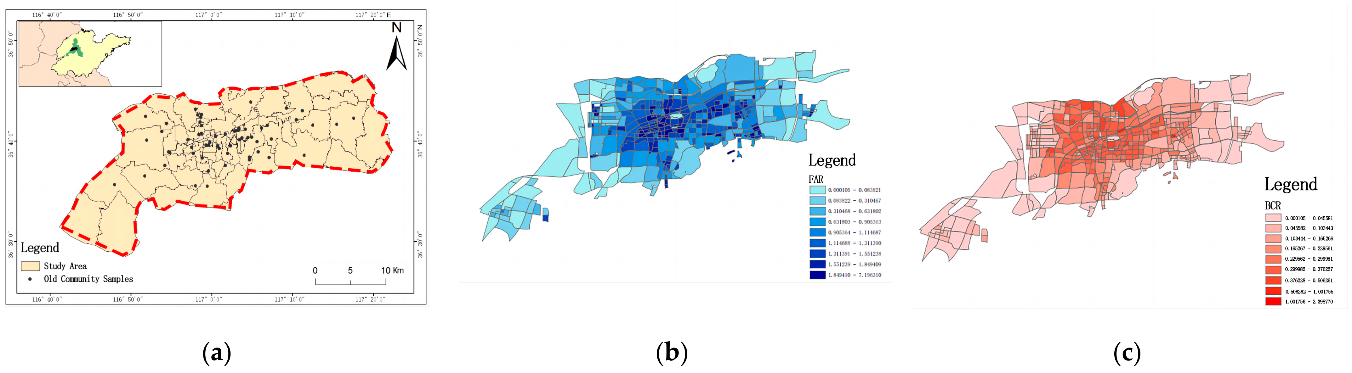
2.1. Study Area
2.2. Methods
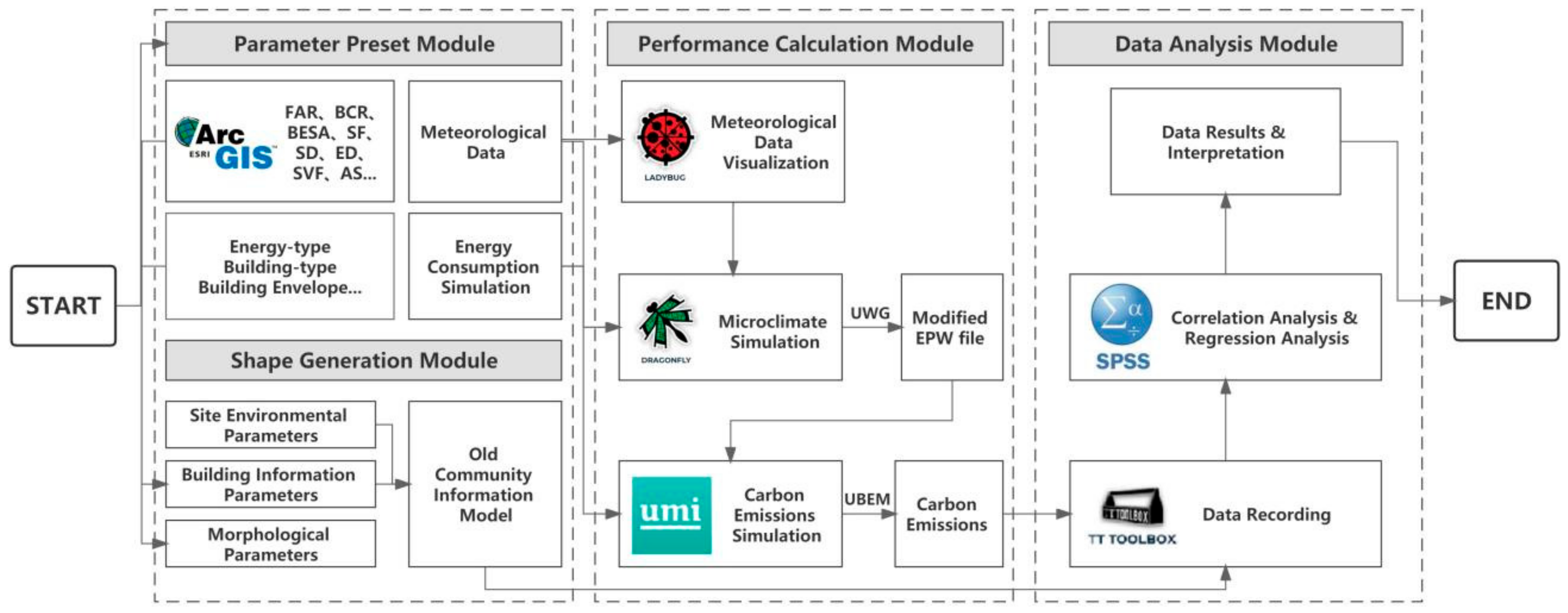
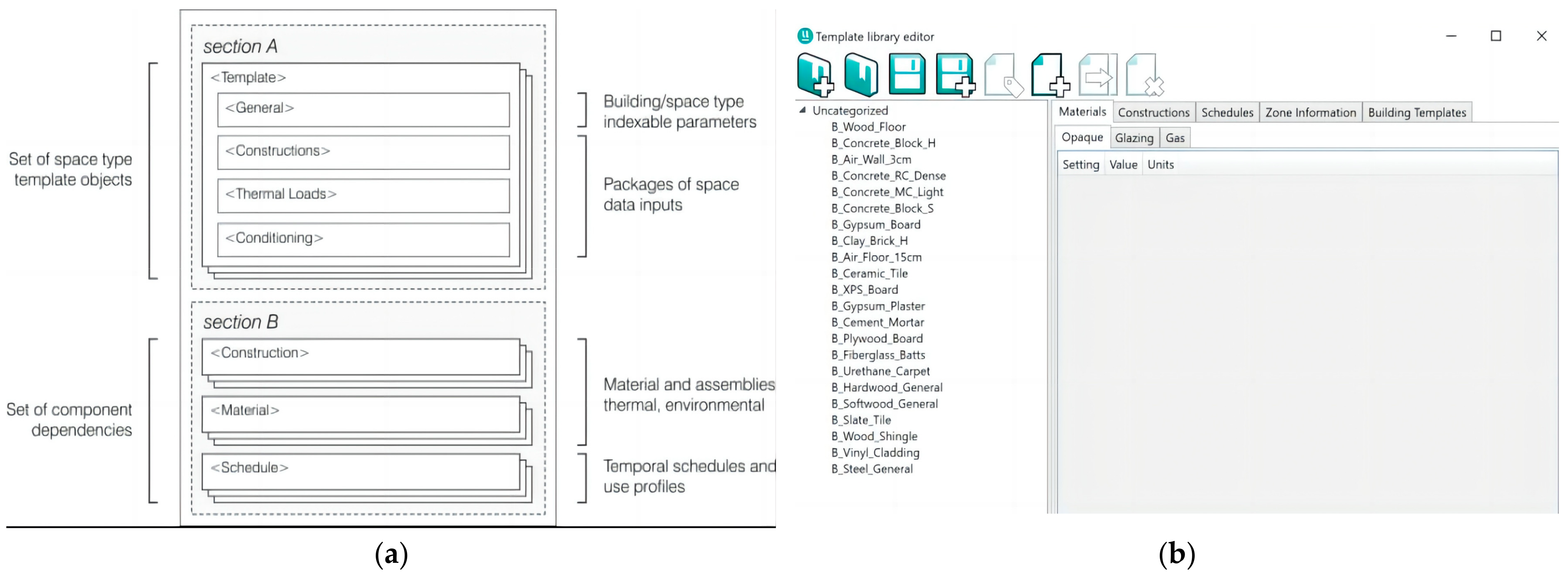
2.2.1. The Construction of Building Information Model
- Acquisition of climate parameters
- Construction of the geometric model of the old community
- Input of building non-geometric attribute information
2.2.2. Extraction and Measurement of Morphological Indices
- Extraction of the morphological indices
- Calculation of morphological indices
2.2.3. Carbon Emission Simulation
- Simulation parameter setting
- Simulation result
2.2.4. Statistical Analyses
- Correlation analysis
- Multiple linear regression analysis
3. Results
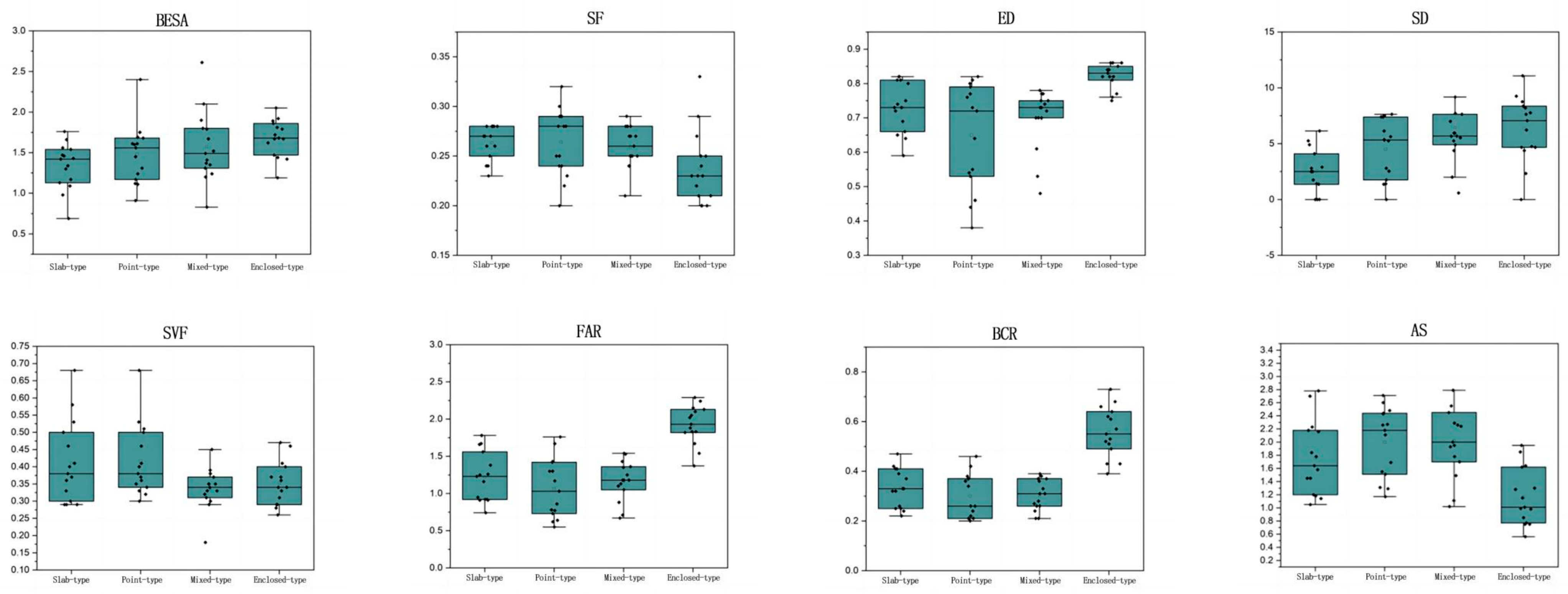
3.1. Spatial Morphological Indices
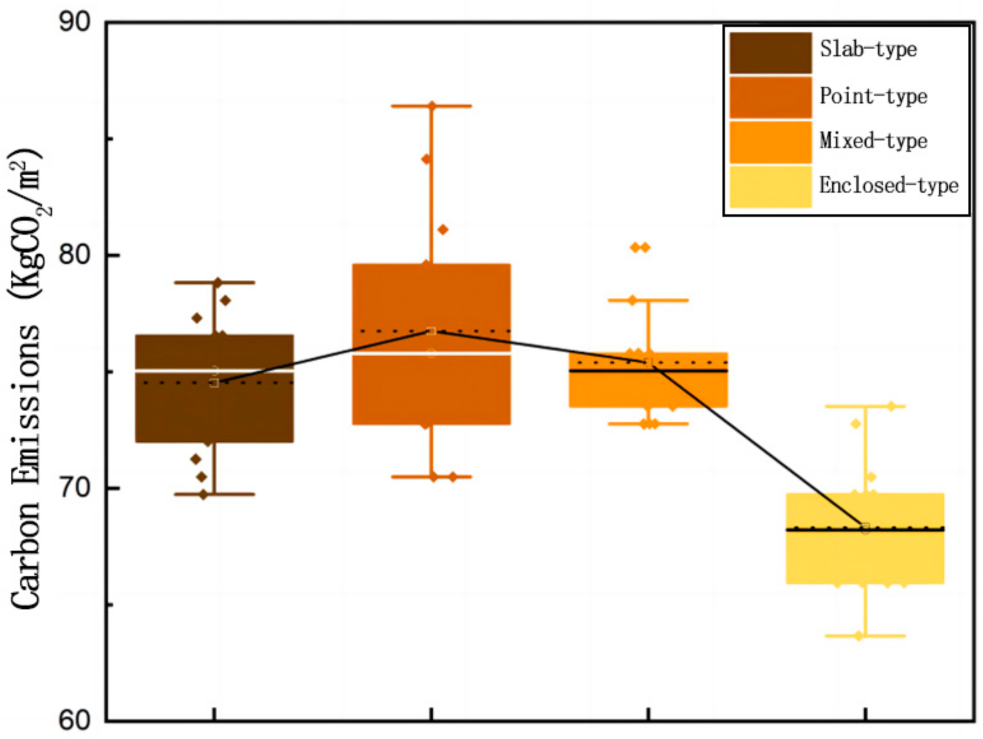
3.2. Results of the Carbon Emission Simulation
3.3. Statistical Analysis
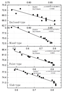
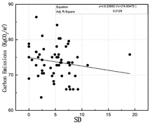
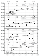
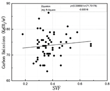
3.3.1. Correlations between Morphological Indices and Carbon Emission
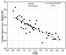
- FAR
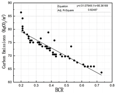
- BCR
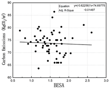
- BESA
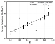
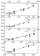
- SF
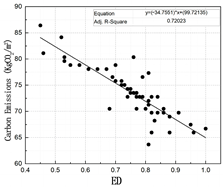
- ED
- SD
- AS
- SVF
3.3.2. Regression Analysis of the Morphological Indices and Carbon Emission
- Establishing the correlation indices
- Multiple linear regression analysis
4. Discussion
4.1. Result Analysis
4.1.1. Impact of Morphological Density Indices on Carbon Emission
4.1.2. Impact of Morphological Texture Indices on Carbon Emissions
4.1.3. Impact of Morphological Layout Type on Carbon Emissions
4.2. Perspectives
5. Conclusions
- Of the four types of building groups outlined in this research, namely point-type, slab-type, mixed-type and enclosed-type, it was found that the total carbon emissions of the point-type and mixed-type building groups were relatively high, while the carbon emissions of the slab-type building group fell in the middle. Conversely, the carbon emissions per unit area of the enclosed-type building group were relatively low;
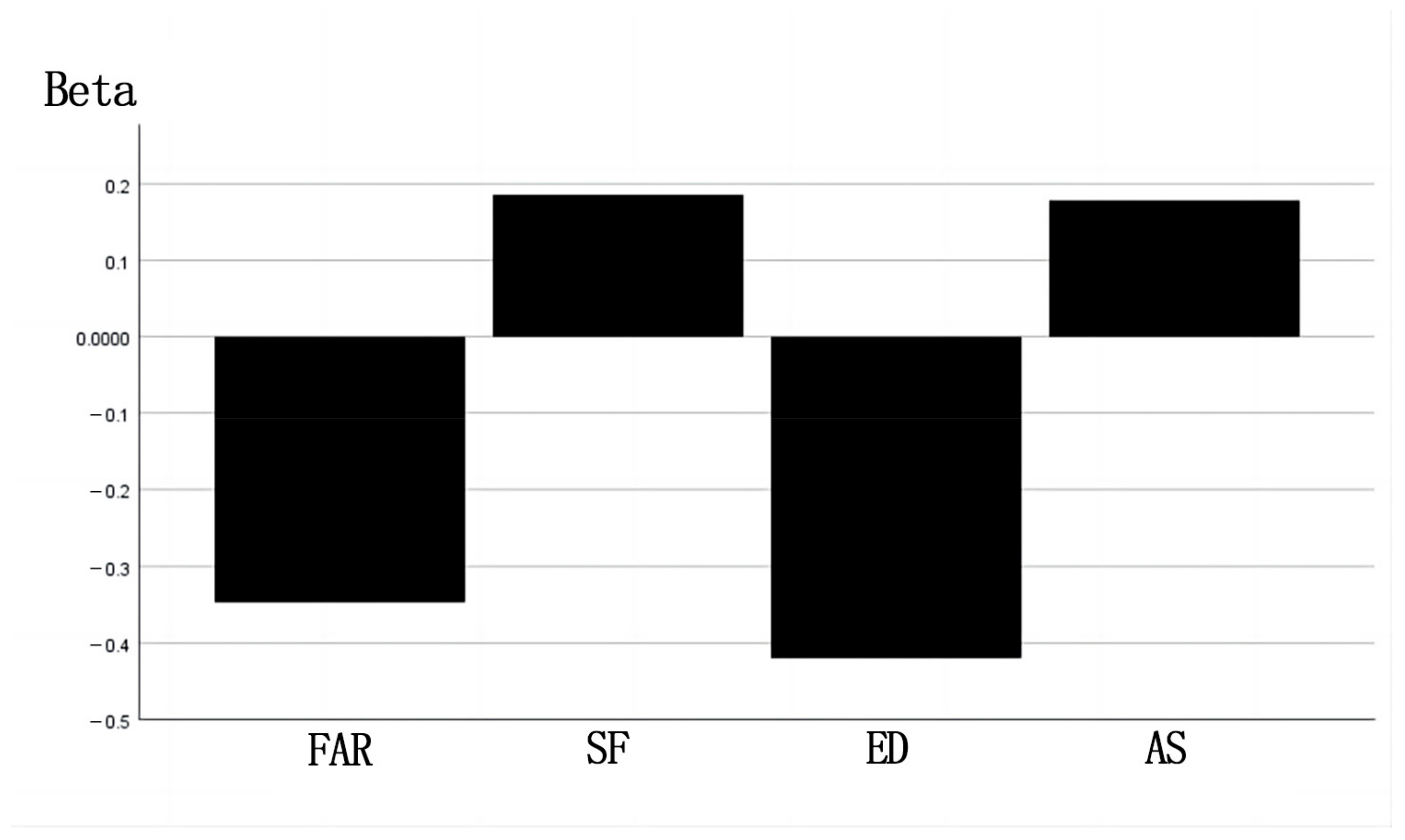
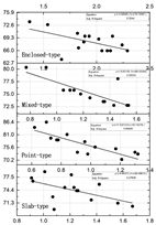
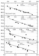
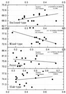
- Among the morphological density and texture indices, the FAR, BCR and ED have obvious negative correlation with the carbon emission of old communities, while the SF and AS are positively correlated with the carbon emission of old communities and have different degrees of influence on different layout types of old communities. Specifically, FAR and ED play a pivotal role in shaping point-type communities, although their influence on enclosed-type communities is minimal. BCR and SF have the greatest influence on point-type communities and the least influence on enclosed-type communities. In addition, AS only has an obvious impact on old communities with an enclosed layout. The other morphological indices have a weak impact on the carbon emissions of the old communities;
- A multiple linear regression analysis was performed to develop a statistical predictive model of carbon emissions in old communities. The fitted equation yielded an R2 value of 0.855, signifying that the variations in independent variables, such as FAR, SF, ED and AS, can account for up to 85.5% of the variance in carbon emissions per unit area of the dependent variable;
- FAR and ED are the primary indices, which significantly impact carbon emissions in old communities, with ED demonstrating the most pronounced effect. Keeping all other indices constant, each unit increase in FAR results in a 3.7% reduction in the carbon emission per unit area, while a unit increase in ED leads to an even greater reduction of 17.1%;
- In essence, enhancing the spatial morphology of built environments in cold regions is a crucial factor in bolstering the carbon reduction potential of older communities in these areas.
Author Contributions
Funding
Data Availability Statement
Acknowledgments
Conflicts of Interest
References
- Laurent Fabius, Opening Speech by Laurent Fabius—Paris Climate Conference. 2015. Available online: http://www.diplomatie.gouv.fr/en/french-foreign-policy/climate/events/ (accessed on 2 May 2023).
- ISO 14064-1:2018; Greenhouse Gases-Part 1: Specification with Guidance at the Organization Level for Quantification and Reporting of Greenhouse Gas Emissions and Removals. ES-UNE: Madrid, Spain, 2018.
- ISO 14064-2:2019; Greenhouse Gases—Part 2: Specification with Guidance at the Project Level for Quantification, Monitoring and Reporting of Greenhouse Gas Emission Reductions or Removal Enhancements. ES-UNE: Madrid, Spain, 2019.
- ISO 14064-2:2019; Greenhouse Gases—Part 3: Specification with Guidance for the Verification and Validation of Greenhouse Gas Statements. ES-UNE: Madrid, Spain, 2019.
- Cano, N.; Berrio, L.; Carvajal, E.; Arango, S. Assessing the carbon footprint of a Colombian University Campus using the UNE-ISO 14064–1 and WRI/WBCSD GHG Protocol Corporate Standard. Environ. Sci. Pollut. Res. 2023, 30, 3980–3996. [Google Scholar] [CrossRef]
- United States Environmental Protection Agency. Overview of Greenhouse Gases; United States Environmental Protection Agency: Washington, DC, USA, 2014.
- Hui, E.C.; Liang, C.; Yip, T.L. Impact of semi-obnoxious facilities and urban renewal strategy on subdivided units. Appl. Geogr. 2018, 91, 144–155. [Google Scholar] [CrossRef]
- Cubi, E.; Doluweera, G.; Bergerson, J. Incorporation of electricity GHG emissions intensity variability into building environmental assessment. Appl. Energy 2015, 159, 62–69. [Google Scholar] [CrossRef]
- Fang, C.L.; Wang, S.J.; Li, G.D. Changing urban forms and carbon dioxide emissions in China: A case study of 30 provincial capital cities. Appl. Energy 2015, 158, 519–531. [Google Scholar] [CrossRef]
- Wang, S.; Fang, C.; Wang, Y.; Huang, Y.; Ma, H. Quantifying the relationship between urban development intensity and carbon dioxide emissions using a panel data analysi. Ecol. Indic. 2015, 49, 121–131. [Google Scholar] [CrossRef]
- Ishii, S.; Tabushi, S.; Aramaki, T.; Hanaki, K. Impact of future urban form on the potential to reduce greenhouse gas emissions from residential, commercial and public buildings in Utsunomiya, Japan. Energy Policy 2010, 38, 4888–4896. [Google Scholar] [CrossRef]
- Kim, J.; Brownstone, D. The impact of residential density on vehicle usage and fuel consumption: Evidence from national samples. Energy Econ. 2013, 40, 196–206. [Google Scholar] [CrossRef]
- Burgalassi, D.; Luzzati, T. Urban spatial structure and environmental emissions: A survey of the literature and some empirical evidence for Italian NUTS 3 regions. Cities 2015, 49, 134–148. [Google Scholar] [CrossRef]
- Lee, S.; Lee, B. The influence of urban form on GHG emissions in the U.S. household sector. Energy Policy 2014, 68, 534–549. [Google Scholar] [CrossRef]
- Hachem, C. Impact of neighborhood design on energy performance and GHG emissions. Appl. Energy 2016, 177, 422–434. [Google Scholar] [CrossRef]
- Grubler, A.; Bai, X.; Buettner, T.; Dhakal, S.; Fisk, D.; Ichinose, T.; Keirstead, J.; Sammer, G.; Satterthwaite, D.; Schulz, N.; et al. Urban energy systems. In Glob Energy Assess—Toward a Sustainable Future; Cambridge University Press: Cambridge, UK, 2012. [Google Scholar]
- UNEP-DTIE Sustainable Consumption and Production Branch. In Cities and Buildings; UNEP: Nairobi, Kenya, 2016.
- IEA. Buildings-Tracking Clean Energy Progress. 2019. Available online: https://www.iea.org/tcep/buildings/ (accessed on 25 March 2019).
- Energy Consumption Statistics Committee of China Building Energy Conservation Association. Research Report on Building Energy Consumption in China; Energy Consumption Statistics Committee of China Building Energy Conservation Association: Xiamen, China, 2022. [Google Scholar]
- Roldán-Fontana, J.; Pacheco-Torres, R.; Jadraque-Gago, E.; Ordónez, J. Optimization of CO2 emissions in the design phases of urban planning, based on geometric characteristics: A case study of a low-density urban area in Spain. Sustain. Sci. 2015, 12, 65–85. [Google Scholar] [CrossRef]
- Cuéllar-Franca, R.M.; Azapagic, A. Environmental impacts of the UK residential sector: Life cycle assessment of houses. Build. Environ. 2012, 54, 86–99. [Google Scholar] [CrossRef]
- Huang, P.J.; Cui, H.; Song, J.L.; Yu, H.Y. Research on carbon emission accounting of buildings in Shanghai. J. Shanghai Univ. Sci. Technol. 2022, 44, 343–350. [Google Scholar]
- Chen, S.; Cui, D.G.; Zhang, H.J. Building carbon emission calculation method and case study. J. Beijing Polytech. 2016, 42, 594–600. [Google Scholar]
- Li, J.; Liu, Y. Carbon emission calculation model of construction project based on the whole life cycle. J. Eng. Manag. 2015, 29, 12–16. [Google Scholar]
- She, J.Q.; Zhang, Y.B.; Qi, S.J. Life-cycle carbon emission characteristics and emission reduction strategies of public buildings in hot summer and warm winter zone—A case study of Xiamen City. Build. Sci. 2014, 30, 13–18. [Google Scholar]
- Zhou, N.; McNeil, M.A.; Levine, M. Energy for 500 Million Homes: Drivers and Outlook for Residential Energy Consumption in China; Lawrence Berkeley National Laboratory: Berkeley, CA, USA, 2009.
- Madlener, R.; Sunak, Y. Impacts of urbanization on urban structures and energy demand: What can we learn for urban energy planning and urbanization management? Sustain. Cities Soc. 2011, 1, 45–53. [Google Scholar] [CrossRef]
- Chen, J.L.; Li, Z.W.; Wang, X.; Ruan, Y.J. Research on the optimization strategy of northern residential area form based on energy consumption survey. Build. Energy Effic. 2018, 46, 8–14. [Google Scholar]
- Yang, X.; Jiang, Y. Comparison of building energy consumption between China and foreign countries. Energy China 2007, 29, 21–26. [Google Scholar]
- Zhang, J.; Yang, Y.; Chen, X.; Mao, Q.Z. Study on the impact of residential built environment on household travel energy consumption in Jinan City. Urban Dev. Stud. 2013, 20, 83–89. [Google Scholar]
- Liu, Z.; Chen, X.F.; Li, S.X. Ambient Microclimate: Collaborative Evaluation Process for Outdoor Thermal Comfort in the Early Design Stage. Chin. Overseas Archit. 2023, 42–48. [Google Scholar]
- Jin, H.; Cui, P. Research on the correlation between morphological elements and temperature of Harbin Central Street commercial district. Build. Sci. 2019, 35, 11–17. [Google Scholar]
- Wei, X. Research on Reducing Carbon Consumption in Residential Community Spaces as Influenced by Microclimate Environments. J. Urban Plan. Dev. 2021, 147, 04021037. [Google Scholar] [CrossRef]
- Yang, P.R.; Quan, J.G. Eco-volume ratio (EAR): Energy consumption assessment and carbon reduction method for urban redevelopment in high-density environment. Urban Plan. Forum 2014, 3, 61–70. [Google Scholar]
- Zhu, R.; Wong, M.S.; You, L.; Santi, P.; Nichol, J.; Ho, H.C.; Lu, L.; Ratti, C. The effect of urban morphology on the solar capacity of threedimensional cities. Renew. Energy 2020, 153, 1111–1126. [Google Scholar] [CrossRef]
- Zhu, R.; You, L.; Santi, P.; Wong, M.S.; Ratti, C. Solar accessibility in developing cities: A case study in Kowloon East, Hong Kong. Sustain. Cities Soc. 2019, 51, 101738. [Google Scholar] [CrossRef]
- Vermeulen, T.; Merino, L.; Knopf-Lenoir, C.; Villon, P.; Beckers, B. Periodic urban models for optimization of passive solar irradiation. Sol. Energy 2018, 162, 67–77. [Google Scholar] [CrossRef]
- Hachem, C.; Fazio, P.; Athienitis, A. Solar optimized residential neighborhoods: Evaluation and design methodology. Sol. Energy 2013, 95, 42–64. [Google Scholar] [CrossRef]
- De Lemos Martinsa, T.A.; Adolphe, L.; Bastos, L.E.G.; de Lemos Martins, M.A. Sensitivity analysis of urban morphology factors regarding solar energypotential of buildings in a Brazilian tropical context. Sol. Energy 2016, 137, 11–24. [Google Scholar] [CrossRef]
- Krüger, E.; Pearlmutter, D.; Rasia, F. Evaluating the impact of canyon geometry and orientation on cooling loads in a high-mass building in a hot dry environment. Appl. Energy 2010, 87, 2068–2078. [Google Scholar] [CrossRef]
- Tsirigoti, D.; Bikas, D. A cross scale analysis of the relationship between energy efficiency and urban morphology in the Greek city context. Procedia Environ. Sci. 2017, 38, 682–687. [Google Scholar] [CrossRef]
- Li, C.; Song, Y.; Kaza, N. Urban form and household electricity consumption: A multilevel study. Energy Build. 2018, 158, 181–193. [Google Scholar] [CrossRef]
- Ahn, Y.J.; Sohn, D.W. The effect of neighbourhood-level urban form on residential building energy use: A GIS-based model using building energy benchmarking data in Seattle. Energy Build. 2019, 196, 124–133. [Google Scholar] [CrossRef]
- Mouzourides, P.; Kyprianou, A.; Neophytou, M.K.A.; Ching, J.; Choudhary, R. Linking the urban-scale building energy demands with city breathability and urban form characteristics. Sustain. Cities Soc. 2019, 49, 101460. [Google Scholar] [CrossRef]
- Swan, L.G.; Ugursal, V.I. Modeling of end-use energy consumption in the residential sector: A review of modeling techniques. Renew. Sustain. Energy Rev. 2009, 13, 1819–1835. [Google Scholar] [CrossRef]
- Howard, B.; Parshall, L.; Thompson, J.; Hammer, S.; Dickinson, J.; Modi, V. Spatial distribution of urban building energy consumption by end use. Energy Build. 2012, 45, 141–151. [Google Scholar] [CrossRef]
- Das, A.; Paul, S.K. CO2 emissions from household consumption in India between 1993–94 and 2006–07: A decomposition analysis. Energy Econ. 2014, 41, 90–105. [Google Scholar] [CrossRef]
- Robinson, D.; Campbell, N.; Gaiser, W.; Kabel, K.; Le-Mouel, A.; Morel, N.; Page, J.; Stankovic, S.; Stone, A. SUNtool–A new modelling paradigm for simulating and optimising urban sustainability. Sol. Energy 2007, 81, 1196–1211. [Google Scholar] [CrossRef]
- Robinson, D.; Haldi, F.; Leroux, P.; Perez, D.; Rasheed, A.; Wilke, U. CitySim: Comprehensive micro-simulation of resource flows for sustainable urban planning. In Proceedings of the Eleventh International IBPSA Conference, Glasgow, UK, 27–30 July 2009; pp. 1083–1090. [Google Scholar]
- Abbasabadi, N.; Ashayeri, M. Urban energy use modeling methods and tools: A review and an outlook. Build. Environ. 2019, 161, 106270. [Google Scholar] [CrossRef]
- Xu, X.; Taylor, J.E.; Pisello, A.L.; Culligan, P.J. The impact of place-based affiliation networks on energy conservation: An holistic model that integrates the influence of buildings, residents and the neighborhood context. Energy Build. 2012, 55, 637–646. [Google Scholar] [CrossRef]
- Letellier-Duchesne, S.; Nagpal, S.; Kummert, M.; Reinhart, C. Balancing demand and supply: Linking neighborhood-level building load calculations with detailed district energy network analysis models. Energy 2018, 150, 913–925. [Google Scholar] [CrossRef]
- Pont, M.B.; Haupt, P. The relation between urban form and density M. Berghauser Pont and P. Haupt. Urban Morphol. 2007, 11, 62–65. [Google Scholar] [CrossRef]
- Ratti, C.; Baker, N.; Steemers, K. Energy consumption and urban texture. Energy Build. 2005, 37, 762–776. [Google Scholar] [CrossRef]
- Liu, K. Energy Efficiency-Driven Urban form Optimization Strategy in Hot Summer and Cold Winter Areas: A Case Study of Residential Blocks in Jianhu County; Southeast University: Nanjing, China, 2022. [Google Scholar]
- Leng, H.; Xiao, Y.T. The influence of residential area form on residential energy consumption in cold city. J. Harbin Inst. Technol. 2020, 52, 147–156+163. [Google Scholar]
- JGJ26-2018; Design Standard for Energy Efficiency of Residential Buildings in Severe Cold and Cold Zones. China Architecture & Building Press: Beijing, China, 2018.
- GB50736-2012; Design Code for Heating Ventilation and Air Conditioning of Civil Buildings. China Architecture & Building Press: Beijing, China, 2012.
- JGJ/T449-2018; Standard for Green Performance Calculation of Civil Buildings. China Architecture & Building Press: Beijing, China, 2018.
- Dong, N. Research on Low-Carbon Renewal Strategy of Old Residential Areas in Tianjin Based on Carbon Emission Accounting; Tianjin University: Tianjin, China, 2021. [Google Scholar]
- Privitera, R.; Palermo, V.; Martinico, F.; Fichera, A.; La Rosa, D. Towards lower carbon cities: Urban morphology contribution in climate change adaptation strategies. Eur. Plan. Stud. 2018, 26, 812–837. [Google Scholar] [CrossRef]
- Yang, F.; Jiang, Z.D. Urban Building Cluster Energy Simulation (UBEM) and Environmentally Sustainable Oriented Urban Planning and Design: Methods, Tools and Paths. Build. Sci. 2019, 37, 17–24. [Google Scholar]
- Leng, H.; Chen, X.; Ma, Y.H. Research progress and enlightenment of the influence of urban form on building energy consumption. Archit. J. 2020, 617, 20–126. [Google Scholar]


| Morphological Indices | Formula | Connotation | Extraction Method | Schematic Diagram |
|---|---|---|---|---|
| Floor Area Ration (FAR) | FAR = Gross Floor Area/Site Area Reflects the spatial distribution characteristics of buildings | FAR = Gross Floor Area/Site Area Reflects the spatial distribution characteristics of buildings | UMI-Site Module |  |
| Building Coverage Ratio (BCR) | BCR = Floor Space/Site Area | Reflects the density of urban or regional buildings |  | |
| Building Exterior Surface Area (BESA) | BESA = Building Exterior Surface Area/Site Area | Reflects the ability of the outer surface of the building to absorb solar radiation | Grasshopper Module |  |
| Shape Factor (SF) | SF = Building Exterior Surface Area/Volume | Reflects the complexity of the building form and the surface area of the enclosure structure |  | |
| Enclosure Degree (ED) | ED = Building Façade Length/Building Control-Line Length | Reflects the openness and closure of a region or space | - | |
| Scattered Degree (SD) | SD = Height Max-Height Average | Reflects the degree of dispersion of buildings in an area or space | - | |
| Average Road Aspect Ratio (AS) | AS = Height Average /Road Width | Reflects the basic morphological unit formed by buildings and roads on both sides of the road in the plot |  | |
| Sky View Factor (SVF) | - | Reflects the shielding degree of building density, height and shape from the surrounding environment | ShadingMask Module |  |
| Type | Samples | ||||
|---|---|---|---|---|---|
| Slab-type |  |  |  |  | … |
| Point-type |  |  |  |  | … |
| Mixed-type |  |  |  |  | … |
| Enclosed-type |  |  |  |  | … |
| Enclosure Structure | Exterior Wall | Floor Slab | Window | Roof | Partition Wall |
|---|---|---|---|---|---|
| Heat Transfer Coefficient (W/(m2·K)) | 1.6 | 1.5 | 3.0 (SHGC = 0.6; South/North Window–Wall Ratio = 0.35; East/West Window–Wall Ratio = 0) | 1.0 | 1.0 |
| Parameter Type | Parameter Settings | ||
|---|---|---|---|
| HVAC System | Type | Domestic Split Air Conditioner | |
| Natural Gas Heating | |||
| Energy Efficiency | Refrigeration Energy Efficiency Ratio | 2.3 | |
| Heating Energy Efficiency Ratio | 1.9 | ||
| Temperature | Refrigeration | 7:00 am–8:00 pm, 20 °C 8:00 pm–7:00 am, 18 °C | |
| Heating | 7:00 am–8:00 pm, 26 °C 8:00 pm–7:00 am, 27 °C | ||
| Occupants | Density | 0.025 per/m2 | |
| Indoor Activity | 7:00 pm–8:00 am, 1 h 8:00 am–9:00 am and 6:00 pm–7:00 pm, 0.7 h 9:00 am–6:00 pm, 0.3 h | ||
| Domestic Water | Time Period | 7:00 am–12:am and 9:00 pm–11:00 pm, 1 h 12:00 am–1:00 pm, 0.6 h 6:00 pm–9:00 pm, 0.2 h | |
| Lighting System | Illuminance | 200 lux | |
| Lighting Power Density | 7 W/m2 | ||
| Illuminating Period | 7:00 am–8:00 am and 10:00 am–12:00 am and 11:00 pm–12:00 pm, 0.2 h 8:00 am–10:00 am and 7:00 pm–8:00 pm, 0.5 h 8:00 pm–12:00 pm, 0.8 h | ||
| Equipment System | Power | 5 W/m2 | |
| Time Period | 1:00 am–6:00 am, 0.2 h 7:00 am–8:00 am and 6:00 pm and 11:00 pm–12:00 pm, 0.6 h 9:00 pm–11:00 pm, 0.8 h 7:00 pm–9:00 pm, 1 h | ||
| Energy Consumption Unit | Factor | Source | Carbon Emission Units | |
|---|---|---|---|---|
| Electrical Energy | kWh/month | 0.758 | Ministry of Science and Technology of China | KgCO2/kWh |
| Combustion Gas | m3/month | 0.232 | Ministry of Science and Technology of China | KgCO2/kWh |
| Domestic Water | t/month | 2.77 | The China Energy Management Network | KgCO2/m3 |
| BESA | SF | ED | SD | SVF | FAR | BCR | AS | |
|---|---|---|---|---|---|---|---|---|
| A-1 | 0.98 | 0.26 | 0.74 | 2.50 | 0.29 | 1.25 | 0.32 | 1.45 |
| A-2 | 1.30 | 0.25 | 0.81 | 4.10 | 0.40 | 1.36 | 0.39 | 1.2 |
| A-3 | 1.46 | 0.24 | 0.8 | 2.50 | 0.38 | 1.67 | 0.41 | 1.84 |
| A-4 | 1.43 | 0.28 | 0.82 | 2.90 | 0.29 | 1.07 | 0.37 | 1.14 |
| A-5 | 1.42 | 0.27 | 0.72 | 4.90 | 0.29 | 1.42 | 0.42 | 1.43 |
| A-6 | 0.69 | 0.28 | 0.7 | 0 | 0.58 | 1.01 | 0.22 | 1.88 |
| A-7 | 1.66 | 0.27 | 0.73 | 0 | 0.30 | 1.16 | 0.26 | 1.64 |
| A-8 | 1.47 | 0.24 | 0.81 | 2.50 | 0.33 | 1.56 | 0.41 | 1.15 |
| A-9 | 1.34 | 0.28 | 0.69 | 1.4 | 0.37 | 0.92 | 0.25 | 1.18 |
| A-10 | 1.54 | 0.26 | 0.67 | 0 | 0.41 | 1.21 | 0.24 | 1.82 |
| A-11 | 1.56 | 0.28 | 0.81 | 2.8 | 0.36 | 0.91 | 0.25 | 1.05 |
| A-12 | 1.13 | 0.27 | 0.73 | 5.25 | 0.5 | 1.23 | 0.32 | 1.45 |
| A-13 | 1.09 | 0.28 | 0.79 | 1.36 | 0.53 | 0.92 | 0.33 | 1.58 |
| A-14 | 1.17 | 0.26 | 0.75 | 6.13 | 0.68 | 1.26 | 0.33 | 1.71 |
| A-15 | 1.76 | 0.23 | 0.82 | 0 | 0.46 | 1.08 | 0.47 | 1.62 |
| B-1 | 1.61 | 0.29 | 0.45 | 1.40 | 0.37 | 0.70 | 0.20 | 2.18 |
| B-2 | 1.24 | 0.29 | 0.55 | 0 | 0.41 | 0.77 | 0.22 | 1.51 |
| B-3 | 1.11 | 0.24 | 0.81 | 2.80 | 0.36 | 1.21 | 0.42 | 1.49 |
| B-4 | 1.75 | 0.28 | 0.64 | 5.25 | 0.50 | 0.96 | 0.24 | 2.13 |
| B-5 | 1.12 | 0.24 | 0.8 | 1.36 | 0.53 | 1.32 | 0.37 | 2.26 |
| B-6 | 0.91 | 0.25 | 0.77 | 6.13 | 0.68 | 1.3 | 0.34 | 1.05 |
| B-7 | 1.69 | 0.32 | 0.73 | 1.75 | 0.46 | 1.17 | 0.26 | 1.17 |
| B-8 | 2.40 | 0.22 | 0.46 | 2.53 | 0.51 | 0.84 | 0.21 | 2.27 |
| B-9 | 1.68 | 0.23 | 0.68 | 7.63 | 0.34 | 1.21 | 0.46 | 1.69 |
| B-10 | 1.56 | 0.29 | 0.52 | 5.32 | 0.3 | 0.62 | 0.21 | 2.44 |
| B-11 | 1.61 | 0.25 | 0.76 | 7.4 | 0.35 | 0.91 | 0.36 | 1.31 |
| B-12 | 1.45 | 0.20 | 0.79 | 5.36 | 0.4 | 0.98 | 0.37 | 2.43 |
| B-13 | 1.6 | 0.28 | 0.58 | 7.39 | 0.38 | 0.78 | 0.38 | 1.55 |
| B-14 | 1.31 | 0.28 | 0.72 | 5.62 | 0.32 | 1.03 | 0.26 | 1.14 |
| B-15 | 1.17 | 0.30 | 0.53 | 7.53 | 0.33 | 0.73 | 0.21 | 1.24 |
| C-1 | 1.31 | 0.24 | 0.78 | 5.25 | 0.35 | 1.43 | 0.37 | 1.28 |
| C-2 | 0.83 | 0.28 | 0.7 | 4.90 | 0.38 | 1.05 | 0.26 | 1.36 |
| C-3 | 1.35 | 0.26 | 0.74 | 0.58 | 0.37 | 1.25 | 0.33 | 2.26 |
| C-4 | 2.61 | 0.28 | 0.61 | 7.00 | 0.18 | 1.46 | 0.24 | 1.02 |
| C-5 | 1.49 | 0.27 | 0.73 | 4.38 | 0.35 | 1.18 | 0.28 | 2.79 |
| C-6 | 1.90 | 0.21 | 0.7 | 19.04 | 0.32 | 1.1 | 0.27 | 2.45 |
| C-7 | 2.10 | 0.28 | 0.7 | 2.00 | 0.33 | 1.13 | 0.26 | 2.55 |
| C-8 | 1.37 | 0.25 | 0.75 | 5.95 | 0.34 | 1.35 | 0.36 | 1.11 |
| C-9 | 1.8 | 0.29 | 0.53 | 5.67 | 0.31 | 0.77 | 0.21 | 1.93 |
| C-10 | 1.79 | 0.27 | 0.73 | 9.17 | 0.39 | 1.18 | 0.31 | 1.95 |
| C-11 | 1.67 | 0.25 | 0.77 | 5.68 | 0.45 | 1.53 | 0.38 | 1.49 |
| C-12 | 1.2 | 0.24 | 0.76 | 5.94 | 0.29 | 0.92 | 0.21 | 2.79 |
| C-13 | 1.52 | 0.25 | 0.75 | 7.63 | 0.33 | 1.36 | 0.37 | 2.24 |
| C-14 | 1.24 | 0.27 | 0.72 | 5.53 | 0.35 | 1.18 | 0.31 | 1.7 |
| C-15 | 1.41 | 0.25 | 0.77 | 7.71 | 0.3 | 1.54 | 0.39 | 1.78 |
| D-1 | 1.19 | 0.24 | 0.81 | 2.33 | 0.37 | 1.67 | 0.73 | 0.75 |
| D-2 | 1.86 | 0.27 | 0.83 | 4.67 | 0.29 | 1.88 | 0.55 | 0.99 |
| D-3 | 1.89 | 0.22 | 0.88 | 0.00 | 0.28 | 2.02 | 0.52 | 1.85 |
| D-4 | 2.05 | 0.33 | 0.91 | 4.38 | 0.31 | 2.15 | 0.51 | 0.85 |
| D-5 | 1.92 | 0.20 | 0.86 | 6.22 | 0.33 | 1.89 | 0.49 | 1.64 |
| D-6 | 1.47 | 0.23 | 0.84 | 8.75 | 0.29 | 1.93 | 0.43 | 1.95 |
| D-7 | 1.42 | 0.21 | 0.86 | 4.67 | 0.46 | 1.82 | 0.43 | 1.3 |
| D-8 | 1.67 | 0.29 | 0.84 | 11.08 | 0.26 | 1.54 | 0.39 | 1.62 |
| D-9 | 1.81 | 0.25 | 0.75 | 8.2 | 0.47 | 1.37 | 0.53 | 1.01 |
| D-10 | 1.79 | 0.25 | 0.96 | 7.77 | 0.4 | 2.05 | 0.68 | 0.62 |
| D-11 | 1.62 | 0.23 | 0.82 | 9.25 | 0.37 | 2.13 | 0.66 | 0.76 |
| D-12 | 1.68 | 0.23 | 0.82 | 7.06 | 0.41 | 2.29 | 0.64 | 0.77 |
| D-13 | 1.72 | 0.21 | 0.88 | 8.36 | 0.34 | 2.1 | 0.62 | 0.54 |
| D-14 | 1.44 | 0.20 | 1 | 7.63 | 0.36 | 1.83 | 0.61 | 0.56 |
| D-15 | 1.67 | 0.20 | 0.95 | 4.74 | 0.34 | 2.24 | 0.57 | 0.62 |
| Carbon Emissions (KgCO2/m2) | Carbon Emissions (KgCO2/m2) | Carbon Emissions (KgCO2/m2) | Carbon Emissions (KgCO2/m2) | ||||
|---|---|---|---|---|---|---|---|
| A-1 | 74.28 | B-1 | 86.41 | C-1 | 72.77 | D-1 | 63.67 |
| A-2 | 72.01 | B-2 | 78.83 | C-2 | 75.80 | D-2 | 68.22 |
| A-3 | 70.49 | B-3 | 70.49 | C-3 | 74.28 | D-3 | 68.98 |
| A-4 | 72.77 | B-4 | 78.07 | C-4 | 78.07 | D-4 | 69.74 |
| A-5 | 75.80 | B-5 | 72.77 | C-5 | 75.04 | D-5 | 69.74 |
| A-6 | 78.83 | B-6 | 73.53 | C-6 | 75.80 | D-6 | 69.74 |
| A-7 | 75.04 | B-7 | 75.04 | C-7 | 75.80 | D-7 | 70.49 |
| A-8 | 71.25 | B-8 | 81.11 | C-8 | 73.53 | D-8 | 72.77 |
| A-9 | 76.55 | B-9 | 70.49 | C-9 | 80.35 | D-9 | 73.53 |
| A-10 | 78.07 | B-10 | 84.14 | C-10 | 75.04 | D-10 | 65.95 |
| A-11 | 77.32 | B-11 | 73.53 | C-11 | 72.77 | D-11 | 65.95 |
| A-12 | 75.04 | B-12 | 72.77 | C-12 | 80.35 | D-12 | 65.95 |
| A-13 | 76.56 | B-13 | 78.83 | C-13 | 73.53 | D-13 | 65.95 |
| A-14 | 74.28 | B-14 | 75.80 | C-14 | 75.04 | D-14 | 66.70 |
| A-15 | 69.74 | B-15 | 79.59 | C-15 | 72.77 | D-15 | 67.46 |
| Impact on Carbon Emissions | The Degree of Influence on Four Types of Old Communities | Impact on Carbon Emissions | The Degree of Influence on Four Types of Old Communities |
|---|---|---|---|
 |  |  |  |
 |  |  |  |
 |  |  |  |
 |  |  |  |
| BESA | SF | ED | SD | SVF | FAR | BCR | AS | Carbon Emission | ||
|---|---|---|---|---|---|---|---|---|---|---|
| BESA | Correlation Coefficient | 1 | −0.075 | −0.052 | 0.232 | −0.371 ** | 0.231 | 0.13 | 0.01 | −0.047 |
| Significance | 0.571 | 0.69 | 0.074 | 0.004 | 0.076 | 0.322 | 0.94 | 0.72 | ||
| Numbers | 60 | 60 | 60 | 60 | 60 | 60 | 60 | 60 | 60 | |
| SF | Correlation Coefficient | −0.075 | 1 | −0.453 ** | −0.254 | −0.042 | −0.461 ** | −0.517 ** | 0.044 | 0.547 ** |
| Significance | 0.571 | 0 | 0.05 | 0.751 | 0 | 0 | 0.74 | 0 | ||
| Numbers | 60 | 60 | 60 | 60 | 60 | 60 | 60 | 60 | 60 | |
| ED | Correlation Coefficient | −0.052 | −0.453 ** | 1 | 0.128 | −0.057 | 0.772 ** | 0.736 ** | −0.477 ** | −0.851 ** |
| Significance | 0.69 | 0 | 0.329 | 0.664 | 0 | 0 | 0 | 0 | ||
| Numbers | 60 | 60 | 60 | 60 | 60 | 60 | 60 | 60 | 60 | |
| SD | Correlation Coefficient | 0.232 | −0.254 | 0.128 | 1 | −0.197 | 0.201 | 0.212 | −0.068 | −0.172 |
| Significance | 0.074 | 0.05 | 0.329 | 0.132 | 0.123 | 0.104 | 0.608 | 0.188 | ||
| Numbers | 60 | 60 | 60 | 60 | 60 | 60 | 60 | 60 | 60 | |
| SVF | Correlation Coefficient | −0.371 ** | −0.042 | −0.057 | −0.197 | 1 | −0.16 | −0.076 | 0.025 | 0.064 |
| Significance | 0.004 | 0.751 | 0.664 | 0.132 | 0.221 | 0.565 | 0.852 | 0.629 | ||
| Numbers | 60 | 60 | 60 | 60 | 60 | 60 | 60 | 60 | 60 | |
| FAR | Correlation Coefficient | 0.231 | −0.461 ** | 0.772 ** | 0.201 | −0.16 | 1 | 0.830 ** | −0.525 ** | −0.848 ** |
| Significance | 0.076 | 0 | 0 | 0.123 | 0.221 | 0 | 0 | 0 | ||
| Numbers | 60 | 60 | 60 | 60 | 60 | 60 | 60 | 60 | 60 | |
| BCR | Correlation Coefficient | 0.13 | −0.517 ** | 0.736 ** | 0.212 | −0.076 | 0.830 ** | 1 | −0.600 ** | −0.910 ** |
| Significance | 0.322 | 0 | 0 | 0.104 | 0.565 | 0 | 0 | 0 | ||
| Numbers | 60 | 60 | 60 | 60 | 60 | 60 | 60 | 60 | 60 | |
| AS | Correlation Coefficient | 0.01 | 0.044 | −0.477 ** | −0.068 | 0.025 | −0.525 ** | −0.600 ** | 1 | 0.563 ** |
| Significance | 0.94 | 0.74 | 0 | 0.608 | 0.852 | 0 | 0 | 0 | ||
| Numbers | 60 | 60 | 60 | 60 | 60 | 60 | 60 | 60 | 60 | |
| Carbon Emission | Correlation Coefficient | −0.047 | 0.547 ** | −0.851 ** | −0.172 | 0.064 | −0.848 ** | −0.910 ** | 0.563 ** | 1 |
| Significance | 0.72 | 0 | 0 | 0.188 | 0.629 | 0 | 0 | 0 | ||
| Numbers | 60 | 60 | 60 | 60 | 60 | 60 | 60 | 60 | 60 | |
| Model | R | R2 | Adjusted R2 | Standard Error of Estimate | Durbin–Watson |
|---|---|---|---|---|---|
| 1 | 0.925 | 0.855 | 0.845 | 1.813167 | 1.971 |
| Model | Partial Regression Coefficient | Standardized Regression Coefficient | t | Statistical Significance | Collinearity | |||
|---|---|---|---|---|---|---|---|---|
| B | Standard Error | Beta | Tolerance | VIF | ||||
| 1 | (constant) | 81.927 | 4.21 | 19.458 | 0 | |||
| FAR | − 3.731 | 0.936 | − 0.347 | − 3.987 | 0 | 0.348 | 2.877 | |
| SF | 28.76 | 9.527 | 0.186 | 3.019 | 0.004 | 0.696 | 1.437 | |
| ED | − 17.078 | 3.358 | − 0.42 | − 5.086 | 0 | 0.386 | 2.59 | |
| AS | 1.44 | 0.513 | 0.178 | 2.808 | 0.007 | 0.655 | 1.527 | |
| No. | Layout Type | FAR | SF | ED | AS | Measured Value of Carbon Emission (KgCO2/m2) | Prediction of Carbon Emission (KgCO2/m2) | |
|---|---|---|---|---|---|---|---|---|
| A01 |  | Slab-type | 1.91 | 0.26 | 0.74 | 1.45 | 78.58 | 80.95 |
| A02 |  | Enclosed-type | 1.33 | 0.25 | 0.81 | 1.20 | 75.56 | 77.33 |
| A03 |  | Enclosed-type | 1.51 | 0.24 | 0.82 | 1.84 | 74.49 | 78.05 |
| A04 |  | Slab-type | 1.38 | 0.28 | 0.80 | 1.14 | 71.77 | 78.15 |
| A05 |  | Slab-type | 1.29 | 0.27 | 0.72 | 2.18 | 79.80 | 80.96 |
| A06 |  | Slab-type | 1.30 | 0.25 | 0.77 | 2.71 | 76.43 | 79.96 |
| A07 |  | Slab-type | 1.87 | 0.27 | 0.73 | 1.64 | 80.04 | 81.50 |
| A08 |  | Enclosed-type | 1.36 | 0.24 | 0.81 | 2.70 | 71.25 | 78.91 |
| A09 |  | Point-type | 1.75 | 0.28 | 0.69 | 1.18 | 76.64 | 81.88 |
| A10 |  | Enclosed-type | 1.58 | 0.20 | 0.86 | 1.54 | 73.14 | 76.18 |
| A11 |  | Slab-type | 1.67 | 0.24 | 0.81 | 2.11 | 79.39 | 78.99 |
| A12 |  | Point-type | 1.23 | 0.27 | 0.73 | 1.45 | 75.04 | 79.74 |
| A13 |  | Point-type | 1.09 | 0.28 | 0.66 | 1.58 | 76.56 | 81.50 |
| A14 |  | Slab-type | 1.65 | 0.26 | 0.75 | 2.78 | 78.48 | 81.56 |
| A15 |  | Enclosed-type | 1.78 | 0.23 | 0.82 | 2.23 | 77.74 | 78.97 |
Disclaimer/Publisher’s Note: The statements, opinions and data contained in all publications are solely those of the individual author(s) and contributor(s) and not of MDPI and/or the editor(s). MDPI and/or the editor(s) disclaim responsibility for any injury to people or property resulting from any ideas, methods, instructions or products referred to in the content. |
© 2023 by the authors. Licensee MDPI, Basel, Switzerland. This article is an open access article distributed under the terms and conditions of the Creative Commons Attribution (CC BY) license (https://creativecommons.org/licenses/by/4.0/).
Share and Cite
Zheng, F.; Wang, Y.; Shen, Z.; Wang, Y. Research on the Correlations between Spatial Morphological Indices and Carbon Emission during the Operational Stage of Built Environments for Old Communities in Cold Regions. Buildings 2023, 13, 2222. https://doi.org/10.3390/buildings13092222
Zheng F, Wang Y, Shen Z, Wang Y. Research on the Correlations between Spatial Morphological Indices and Carbon Emission during the Operational Stage of Built Environments for Old Communities in Cold Regions. Buildings. 2023; 13(9):2222. https://doi.org/10.3390/buildings13092222
Chicago/Turabian StyleZheng, Fei, Yuqing Wang, Zhicheng Shen, and Yuetao Wang. 2023. "Research on the Correlations between Spatial Morphological Indices and Carbon Emission during the Operational Stage of Built Environments for Old Communities in Cold Regions" Buildings 13, no. 9: 2222. https://doi.org/10.3390/buildings13092222