Minimum Cost Design for Rectangular Isolated Footings Taking into Account That the Column Is Located in Any Part of the Footing

Abstract

This work presents a new model for obtaining the cheapest design for a rectangular isolated footing, taking into account that the column is located in any part of the footing. The methodology is developed by integration to obtain the moments, bending shear and punching shear according to the American Concrete Institute ACI 318-14. This document presents the simplified and precise equations of the four moments, four bending shears and one punching shear acting on the footing. Some designs have been developed by the trial and error method to determine the footing dimensions, and later the thickness and steel area of the footing are obtained. Some authors present the minimum cost design for a rectangular isolated footing taking into account that the column is located in the center of gravity of the footing, and other authors present very complex algorithms. Numerical examples are presented to obtain the minimum cost design of rectangular isolated footings under biaxial bending, and some results are compared with those of other authors considering the same conditions. The new model presents a smaller contact area with the soil and a lower design cost than those presented by other authors.

1. Introduction

Footing or foundation is the structural member (sub-structure) that transfers the loads of the superstructure to the soil. Footings are used in various types of construction in structural engineering, such as buildings and bridges. The main object of geotechnical and structural engineers is to obtain the smallest area and the minimum cost of the footing to support the loads imposed by the superstructure.

Optimization techniques have been successfully used in various foundation problems, such as in the following: Hannan et al. [1] showed a strategy to obtain minimum volume for reinforced concrete footing that supports a wind load on the superstructure. Basudhar et al. [2,3] investigated the optimal cost design for a rigid raft foundation and circular isolated footings, taking into account the cost of concrete, cost of excavations, cost of backfilling works and cost of steel reinforcement based in the mathematical programming problem using Powell’s conjugate direction search method. Al-Douri [4] proposed an optimal model for the design of trapezoidal combined footings, taking into account the cost of concrete, cost of excavations, cost of backfilling works and cost of steel reinforcement. Wang and Kulhawy [5] proposed the minimum construction cost as the objective function of a foundation considering the serviceability limit state (SLS), ultimate limit state (ULS), and economics. Rizwan et al. [6] developed an optimal design of reinforced concrete combined footings using computational procedure, and the objective function included the cost of excavation, filling, concrete and reinforcement for the footings. Jelušič and Žlender [7,8] developed an optimal design for reinforced pad and strip foundations based on optimizations via multiparametric, mixed-integer, and nonlinear programming (MINLP). Velázquez-Santillán et al. [9] presented a design for reinforced rectangular concrete to obtain the minimum cost design, as well as the optimal radius, thickness, and reinforced steel areas in both directions. López-Chavarría et al. [10] designed a model for circular isolated footings to obtain the minimum cost design, as well as the optimal radius, thickness, and reinforced steel areas in both directions. Khajuria and Singh [11] proposed a metaheuristic optimization for the design of reinforced concrete footings supporting a column based of the gravitational search algorithm (GSA). Al-Ansari and Afzal [12] presented a simplified analysis for the design of irregularly shaped reinforced concrete footings with an eccentric load subject to biaxial bending that supports a square column; the shapes of the footings studied were square, triangular, circular, and trapezoidal. Kashani et al. [13] studied the optimal design of reinforced concrete combined footings according to the American Concrete Institute ACI 318-05, using the five swarm intelligence algorithms of particle swarm optimization (PSO), accelerated particle swarm optimization (APSO), whale optimization algorithm (WOA), ant lion optimizer (ALO), and moth flame optimization (MFO). Nigdeli and Bekdas [14] investigated the orientation of a column mounted on footings using the optimal design-based harmony search algorithm. Kamal et al. [15] presented a study on the optimal design of footing systems applied in the prefabricated industrial buildings, with the concrete bracket system uses as the connection type in the reinforced concrete frames.

The main contributions of the optimization techniques in the design of rectangular isolated footings are as follows: Camp and Assadollahi [16] presented the optimal design of reinforced concrete footings according to the American Concrete Institute ACI 318-11 subjected to vertical load using a hybrid Big Bang–Big Crunch (BB-BC) algorithm. Luévanos-Rojas et al. [17] developed an optimal model for the design of rectangular isolated footings using computation to solve various integrals according to the American Concrete Institute ACI 318-13. Galvis and Smith-Pardo [18] presented design aids and simplified closed-form equations to obtain the coupled axial load and biaxial moment capacity of hollow and solid circular and rectangular shallow foundations. Rawat and Mittal and Rawat et al. [19,20] developed a simplified approach for the design of reinforced concrete rectangular isolated footings with eccentric load according to the American Concrete Institute ACI 318-14. Solorzano and Plevris [21] studied genetic algorithms (GA) with a selection technique applied to the optimal design of reinforced concrete rectangular isolated footings according to the American Concrete Institute ACI 318-19. Chaudhuri and Maity [22] investigated the optimal design of reinforced concrete isolated footings according to the Indian Standard (IS) 456:2000 [23], using the two swarm intelligence algorithms of genetic algorithms (GA) and unified particle swarm optimization (UPSO). Also, metaheuristic optimization has been enthusiastically applied in the design of reinforced concrete rectangular isolated footings as a practical tool in parametric research using different algorithms, such as Harmony Search (HS), the Teaching Learning Based Optimization (TLBO) algorithm and Flower Pollination Algorithm (FPA) [24], as well as the Evolutionary Algorithm (EA) and the Genetic Algorithm (GA) [25].

This study shows a new model for obtaining the minimum cost design for a rectangular isolated footing subjected to biaxial bending by the application of the load and moments of the column, wherein the column is located in any part of the footing. The cheapest design is achieved in two stages. First stage: the objective function is the minimum area of contact with the soil; the known or constant parameters (independent variables) are σ_max, P, e_x. e_y, M_x and M_y; the unknown or decision variables (dependent variables) are A_min, h_x and h_y. Second stage: the objective function is the minimum cost; the known or constant parameters (independent variables) are σ_max, P_u, M_ux and M_uy, h_x and h_y; the unknown or decision variables (dependent variables) are C_min, d, A_sx and A_sy. Numerical examples are shown to find the minimum cost design of rectangular isolated footings subjected to biaxial bending for four examples.

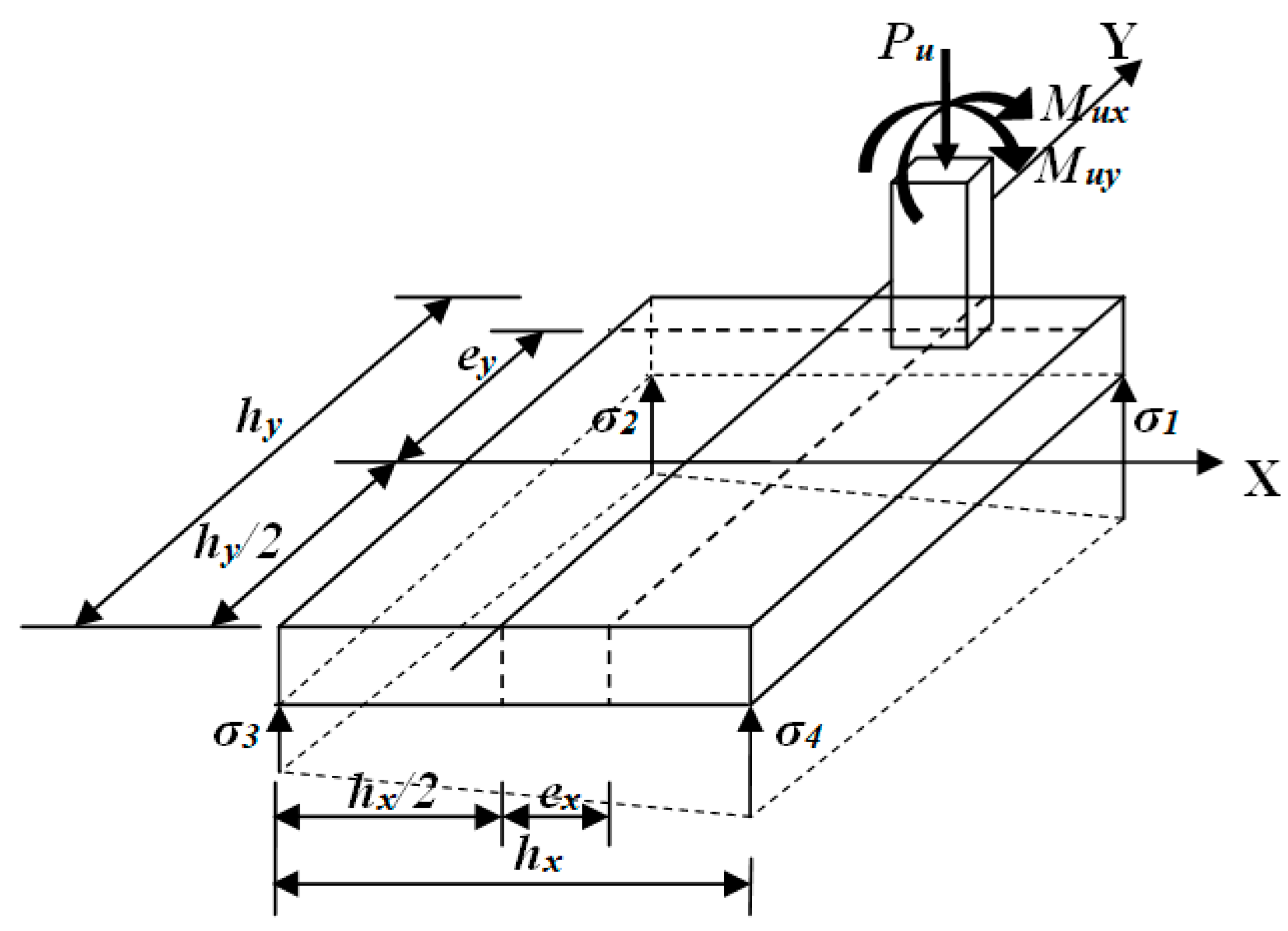
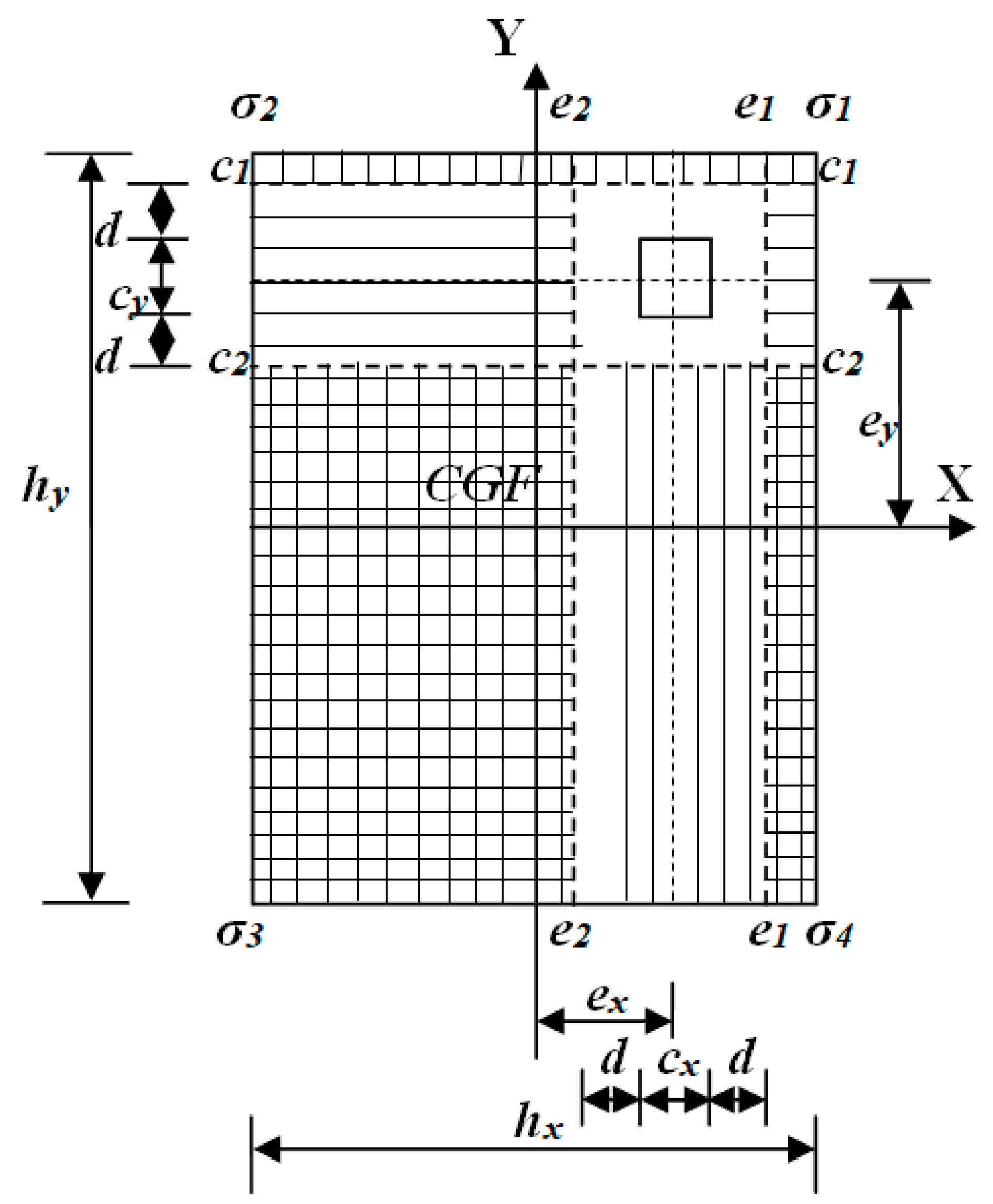
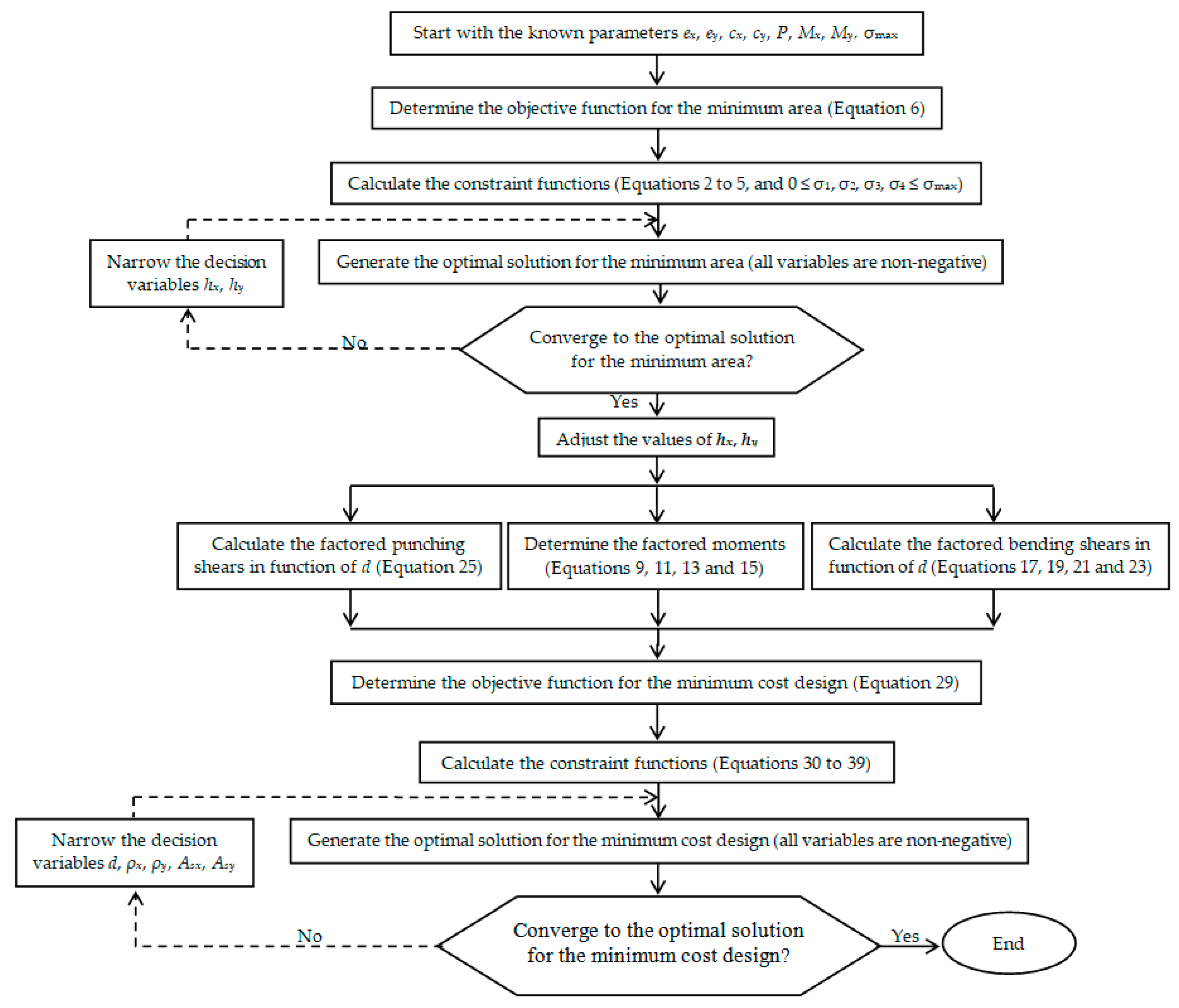
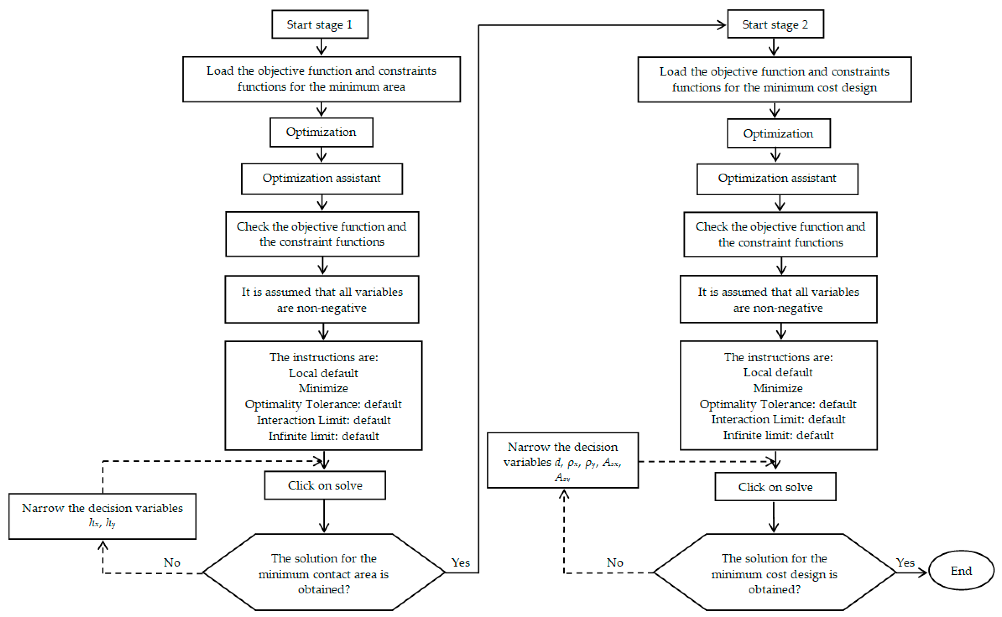
2. Formulation of the Model

The loads and moments are obtained from a structural analysis, whereby the analysis of the structural framework can be undertaken via any of the known methods (stiffness method, slope-deflection method and Hardy Cross method) that include dead, live, wind, and earthquake loads.

Figure 1 shows a rectangular isolated footing subjected to biaxial bending and the column located in any part of the footing on elastic soils, assuming a linear distribution of soil pressure.

General equation for any type of footing subjected to biaxial bending:

$$\sigma =\frac{P}{A}+\frac{M_{xT}y}{I_x}+\frac{M_{yT}x}{I_y},$$

(1)

where σ is the pressure of the soil in any part of the footing, P is the axial load, M_xT and M_yT are the total moments on the X and Y axes, A is the area or surface of contact of the footing with the soil, I_x and I_y are the moments of inertia of the footing on the X and Y axes, and x and y are the coordinates where it is desired to find the soil pressure on the footing.

Equation (1) assumes that the contact area of the footing with the soil works totally under compression.

Now, substituting A = h_xh_y, I_x = h_xh_y³/12, I_y = h_yh_x³/12, M_xT = M_x + Pe_y, M_yT = M_y + Pe_x, and the corresponding coordinates at each corner of the rectangular isolated footing, the pressures are obtained as:

$${\sigma }_1=\frac{P}{h_x{h}_y}+\frac{6\left(M_x+P{e}_y\right)}{h_x{h_y}^2}+\frac{6\left(M_y+P{e}_x\right)}{{h_x}^2{h}_y},$$

(2)

$${\sigma }_2=\frac{P}{h_x{h}_y}+\frac{6\left(M_x+P{e}_y\right)}{h_x{h_y}^2}-\frac{6\left(M_y+P{e}_x\right)}{{h_x}^2{h}_y},$$

(3)

$${\sigma }_3=\frac{P}{h_x{h}_y}-\frac{6\left(M_x+P{e}_y\right)}{h_x{h_y}^2}-\frac{6\left(M_y+P{e}_x\right)}{{h_x}^2{h}_y},$$

(4)

$${\sigma }_4=\frac{P}{h_x{h}_y}-\frac{6\left(M_x+P{e}_y\right)}{h_x{h_y}^2}+\frac{6\left(M_y+P{e}_x\right)}{{h_x}^2{h}_y},$$

(5)

where h_x and h_y are the sides of the footing in the directions X and Y.

2.1. Optimal Area for Rectangular Isolated Footing

The objective function for the minimum area “A_min” is obtained via:

$$A_{min}=h_x{h}_y,$$

(6)

The constraint functions are the Equations (2) to (5), where 0 ≤ σ₁, σ₂, σ₃, σ₄ ≤ σ_max (allowable bearing capacity of the soil).

Note that the base area of the footing will be determined in relation to the unfactored load P, and the unfactored moments M_x and M_y transmitted by footing to the soil.

2.2. Optimal Cost for Rectangular Isolated Footing

We substitute A = h_xh_y, I_x = h_xh_y³/12, I_y = h_yh_x³/12, M_xT = M_ux + P_ue_y, M_yT = M_uy + P_ue_x into Equation (1) to obtain the pressure in function of the coordinates for a rectangular isolated footing. The pressure equation is:

$${\sigma }_u\left(x,y\right)=\frac{P_u}{h_x{h}_y}+\frac{12\left(M_{ux}+P_u{e}_y\right)y}{h_x{h_y}^3}+\frac{12\left(M_{uy}+P_u{e}_x\right)x}{h_y{h_x}^3}.$$

(7)

where P_u is the factored load and M_ux and M_uy are the factored moments on the X and Y axes.

2.2.1. Equations for Moments

Figure 2 shows the critical sections for moments of a rectangular isolated footing subjected to biaxial bending and the column located in any part of the footing. The critical sections for moments are presented on the faces of the columns.

The general equation for the moment on the a₁ axis “M_ua1” is obtained as follows:

$$M_{ua1}=-{\int }_{e_y+\frac{c_y}{2}}^{\frac{h_y}{2}}{\int }_{-\frac{h_x}{2}}^{\frac{h_x}{2}}{\sigma }_u\left(x,y\right)\left(y-e_y-\frac{c_y}{2}\right)dxdy.$$

(8)

By substituting Equation (7) into Equation (8), M_ua1 is obtained:

$$M_{ua1}=-\frac{\left\{P_u{h_y}^2\left[{\left(h_y-c_y\right)}^2-4e_y\left(h_y-e_y-c_y\right)\right]+2\left(P_u{e}_y+M_{ux}\right)\left[2{h_y}^3-3{h_y}^2\left(2e_y+c_y\right)+{\left(2e_y+c_y\right)}^3\right]\right\}}{8{h_y}^3}.$$

(9)

where c_x and c_y are the sides of the column in the directions X and Y.

The general equation for the moment on the a₂ axis “M_ua2” is obtained as follows:

$$M_{ua2}=\frac{P_u{c}_y}{2}+M_{ux}-{\int }_{e_y-\frac{c_y}{2}}^{\frac{h_y}{2}}{\int }_{-\frac{h_x}{2}}^{\frac{h_x}{2}}{\sigma }_u\left(x,y\right)\left(y-e_y+\frac{c_y}{2}\right)dxdy.$$

(10)

By substituting the Equation (7) into Equation (10), M_ua2 is obtained:

$$M_{ua2}=-\frac{\left\{P_u{h_y}^2\left[{\left(h_y-c_y\right)}^2+4e_y\left(h_y+e_y-c_y\right)\right]-2\left(P_u{e}_y+M_{ux}\right)\left[2{h_y}^3+3{h_y}^2\left(2e_y-c_y\right)-{\left(2e_y-c_y\right)}^3\right]\right\}}{8{h_y}^3}.$$

(11)

Using the general equation for the moment on the b₁ axis, “M_ub1” is obtained as follows:

$$M_{ub1}=-{\int }_{-\frac{h_y}{2}}^{\frac{h_y}{2}}{\int }_{e_x+\frac{c_x}{2}}^{\frac{h_x}{2}}{\sigma }_u\left(x,y\right)\left(x-e_x-\frac{c_x}{2}\right)dxdy.$$

(12)

By substituting Equation (7) into Equation (12), M_ub1 is obtained:

$$M_{ub1}=-\frac{\left\{P_u{h_x}^2\left[{\left(h_x-c_x\right)}^2-4e_x\left(h_x-e_x-c_x\right)\right]+2\left(P_u{e}_x+M_{uy}\right)\left[2{h_x}^3-3{h_x}^2\left(2e_x+c_x\right)+{\left(2e_x+c_x\right)}^3\right]\right\}}{8{h_x}^3}.$$

(13)

Using the general equation for the moment on the b₂ axis, “M_ub2” is obtained as follows:

$$M_{ub2}=\frac{P_u{c}_x}{2}+M_{uy}-{\int }_{-\frac{h_y}{2}}^{\frac{h_y}{2}}{\int }_{e_x-\frac{c_x}{2}}^{\frac{h_x}{2}}{\sigma }_u\left(x,y\right)\left(x-e_x+\frac{c_x}{2}\right)dxdy.$$

(14)

By substituting Equation (7) into Equation (14), M_ub2 is obtained:

$$M_{ub2}=-\frac{\left\{P_u{h_x}^2\left[{\left(h_x-c_x\right)}^2-4e_x\left(h_x-e_x-c_x\right)\right]+2\left(P_u{e}_x+M_{uy}\right)\left[2{h_x}^3-3{h_x}^2\left(2e_x+c_x\right)+{\left(2e_x+c_x\right)}^3\right]\right\}}{8{h_x}^3}.$$

(15)

2.2.2. Equations for Bending Shear

Figure 3 shows the critical sections for the bending shear of a rectangular isolated footing subjected to biaxial bending and the column located in any part of the footing. The critical sections for bending shear occur at a distance d (effective depth of footing) from the column faces.

Using the general equation for the bending shear on the c₁ axis, “V_ufc1” is obtained as follows:

$$V_{ufc1}=-{\int }_{e_y+\frac{c_y}{2}+d}^{\frac{h_y}{2}}{\int }_{-\frac{h_x}{2}}^{\frac{h_x}{2}}{\sigma }_u\left(x,y\right)dxdy.$$

(16)

By substituting Equation (7) into Equation (16), V_ufc1 is obtained:

$$V_{ufc1}=-\frac{\left\{P_u{h_y}^2\left[h_y-c_y-2\left(e_y+d\right)\right]+3\left(P_u{e}_y+M_{ux}\right)\left[{h_y}^2-{\left(2e_y+c_y+2d\right)}^2\right]\right\}}{2{h_y}^3}.$$

(17)

Using the general equation for the bending shear on the c₂ axis, “V_ufc2” is obtained as follows:

$$V_{ufc2}=P_u-{\int }_{e_y-\frac{c_y}{2}-d}^{\frac{h_y}{2}}{\int }_{-\frac{h_x}{2}}^{\frac{h_x}{2}}{\sigma }_u\left(x,y\right)dxdy.$$

(18)

By substituting Equation (7) into Equation (18), V_ufc2 is obtained:

$$V_{ufc2}=\frac{\left\{P_u{h_y}^2\left[h_y-c_y+2\left(e_y-d\right)\right]-3\left(P_u{e}_y+M_{ux}\right)\left[{h_y}^2-{\left(2e_y-c_y-2d\right)}^2\right]\right\}}{2{h_y}^3}.$$

(19)

Using the general equation for the bending shear on the e₁ axis, “V_ufe1” is obtained as follows:

$$V_{ufe1}=-{\int }_{-\frac{h_y}{2}}^{\frac{h_y}{2}}{\int }_{e_x+\frac{c_x}{2}+d}^{\frac{h_x}{2}}{\sigma }_u\left(x,y\right)dxdy.$$

(20)

By substituting the Equation (7) into Equation (20), V_ufe1 is obtained:

$$V_{ufe1}=-\frac{\left\{P_u{h_x}^2\left[h_x-c_x-2\left(e_x+d\right)\right]+3\left(P_u{e}_x+M_{uy}\right)\left[{h_x}^2-{\left(2e_x+c_x+2d\right)}^2\right]\right\}}{2{h_x}^3}.$$

(21)

Using the general equation for the bending shear on the e₂ axis, “V_ufe2” is obtained as follows:

$$V_{ufe2}=P_u-{\int }_{-\frac{h_y}{2}}^{\frac{h_y}{2}}{\int }_{e_x-\frac{c_x}{2}-d}^{\frac{h_x}{2}}{\sigma }_u\left(x,y\right)dxdy.$$

(22)

By substituting Equation (7) into Equation (22), V_ufe2 is obtained:

$$V_{ufe2}=\frac{\left\{P_u{h_x}^2\left[h_x-c_x+2\left(e_x-d\right)\right]-3\left(P_u{e}_x+M_{uy}\right)\left[{h_x}^2-{\left(2e_x-c_x-2d\right)}^2\right]\right\}}{2{h_x}^3}.$$

(23)

2.2.3. Equations for Punching Shear

Figure 4 shows the critical section for punching shear of a rectangular isolated footing subjected to biaxial bending and the column located in any part of the footing. The critical section for punching shear arises at a perimeter formed at a distance d/2 from the column faces in two directions.

Using the general equation for the punching shear, “V_up” is obtained as follows:

$$V_{up}=P_u-{\int }_{y_2}^{y_1}{\int }_{x_2}^{x_1}{\sigma }_u\left(x,y\right)dxdy.$$

(24)

By substituting Equation (7) into Equation (24), V_up is obtained:

$$V_{up}=\frac{P_u{h_x}^3{h_y}^3-\left(x_1-x_2\right)\left(y_1-y_2\right)\left\{P_u{h_x}^2{h_y}^2-6\left[\left(P_u{e}_y+M_{ux}\right){h_x}^2\left(y_1+y_2\right)+\left(P_u{e}_x+M_{uy}\right){h_y}^2\left(x_1+x_2\right)\right]\right\}}{{h_x}^3{h_y}^3}.$$

(25)

where x₁, x₂, y₁ and y₂ are the coordinates of the corners of the critical perimeter in the directions X and Y.

2.2.4. Objective Function to Minimize the Cost

The minimum cost “C_min” is equal to the difference between the steel cost and the concrete cost (the cost includes materials and manpower). The minimum cost of a rectangular isolated footing is:

$$C_{min}=V_c{C}_c+{V_s\gamma }_s{C}_s,$$

(26)

where C_min = minimum cost in USD, C_c = ready mix concrete cost in USD/m³, C_s = steel cost in USD/kN, V_c = concrete volume in m³, V_s = steel volume in m³, γ_c = concrete density is 24 kN/m³, γ_s = steel density is 78 kN/m³. Note: the cost of concrete is quoted in m³ and the cost of steel is quoted in kN.

The volumes for a rectangular isolated footing are:

$$V_s=A_{sx}{h}_x+A_{sy}{h}_y,$$

(27)

$$V_c=h_x{h}_y\left(d+r\right),$$

(28)

where r is concrete cover.

By substituting γ_sC_s = αC_c (where α = γ_sC_s/C_c) and Equations (27) and (28) into Equation (26), we can find “C_min”. The following equation is thus obtained:

$$C_{min}=C_c\left[h_x{h}_y\left(d+r\right)+\left(\alpha -1\right)\left(A_{sx}{h}_x+A_{sy}{h}_y\right)\right]$$

(29)

2.2.5. Constraint Functions

The equations for the design of a rectangular isolated footing are shown in Ref. [26].

The equations for the moments are:

$$\left|M_{ua1}\right|,\left|M_{ua2}\right|\le {Ø}_f{f}_{y}d{A}_{sy}\left(1-\frac{A_{sy}{f}_y}{1.7h_{x}d{f^{\prime }}_c}\right),$$

(30)

$$\left|M_{ub1}\right|,\left|M_{ub2}\right|\le {Ø}_f{f}_{y}d{A}_{sx}\left(1-\frac{A_{sx}{f}_y}{1.7h_{y}d{f^{\prime }}_c}\right),$$

(31)

where f_y = specified yield strength of reinforcement of steel (MPa), f′_c = specified compressive strength of the concrete at 28 days (MPa) A_sy = steel area in the Y direction, A_sx = steel area in the X direction, Ø_f = bending strength reduction factor (0.90).

Equations for the bending shear are:

$$\left|V_{ufc1}\right|,\left|V_{ufc2}\right|\le 0.17{Ø}_v\sqrt{{f\prime }_c}{h}_{x}d,$$

(32)

$$\left|V_{ufe1}\right|,\left|V_{ufe2}\right|\le 0.17{Ø}_v\sqrt{{f^{\prime }}_c}{h}_{y}d.$$

(33)

where Ø_v = shear strength reduction factor (0.85).

The equation for the punching shear is:

$$\left|V_{up}\right|\le \left\{\begin{array}{c}0.17{Ø}_v\left(1+\frac{2}{{\beta }_c}\right)\sqrt{{f^{\prime }}_c}{b}_{0}d\\ 0.083{Ø}_v\left(\frac{{\alpha }_{s}d}{b_0}+2\right)\sqrt{{f^{\prime }}_c}{b}_{0}d\\ 0.33{Ø}_v\sqrt{{f^{\prime }}_c}{b}_{0}d\end{array}\right.,$$

(34)

where β_c = relationship of the long side between the short sides of the column; b₀ = perimeter of the punching shear (m); α_s = 20 for corner columns, α_s = 30 for edge columns, and α_s = 40 for interior columns.

The equations for the percentage of reinforcing steel are:

$${\rho }_x,{\rho }_y\le 0.75\left[\frac{0.85{\beta }_1{f^{\prime }}_c}{f_y}\left(\frac{600}{600+f_y}\right)\right],$$

(35)

$${\rho }_x,{\rho }_y\ge \left\{\begin{array}{c}\frac{0.25\sqrt{{f^{\prime }}_c}}{f_y}\\ \frac{1.4}{f_y}\end{array}\right.,$$

(36)

$$0.65\le {\beta }_1=\left(1.05-\frac{{f^{\prime }}_c}{140}\right)\le 0.85,$$

(37)

where ρ_x and ρ_y = percentage of reinforcing steel in the X and Y directions, where β₁ is the factor relating the depth of the equivalent rectangular compressive stress block to neutral axis depth.

The equations for the reinforcing steel are:

$$A_{sy}={\rho }_y{h}_{x}d,$$

(38)

$$A_{sx}={\rho }_x{h}_{y}d.$$

(39)

Figure 5 shows the flowchart of the algorithm for the optimal design procedure of reinforced concrete rectangular isolated footing.

Figure 6 shows the flowchart for the use of Maple software 15 for the optimal design of reinforced concrete rectangular isolated footing.

3. Numerical Problems

Table 1, Table 2, Table 3, Table 4, Table 5, Table 6, Table 7 and Table 8 present the four examples used to obtain the optimal design of rectangular isolated footing subjected to biaxial bending (an axial load, a moment on the X axis and a moment on the Y axis). Example 1: When the column is located at the center of gravity of the footing. Example 2: When the column is located at the limit of the footing in the Y direction. Example 3: When the column is located at the limit of the footing in the X direction. Example 4: When the column is located at the limit of the footing in the X and Y directions or at a corner. The general data for all footings are c_x = c_y = 0.40 m, r = 0.08 m, σ_max = 180 kN/m², f′_c = 21 MPa, f_y = 420 MPa and α = 90.

Table 1 and Table 2 show Example 1 with the conditions of P_D = 500 kN and P_L = 500 kN (Example 1.1), P_D = 400 kN and P_L = 450 kN (Example 1.2), P_D = 500 kN and P_L = 250 kN (Example 1.3), and P_D = 400 kN and P_L = 200 kN (Example 1.4), where M_xD = 150 kN-m, M_xL = 75 kN-m, M_yD = 100 kN-m, M_yL = 50 kN-m, e_x = 0, and e_y = 0 (the column is located at the center of gravity of the footing). Table 1 shows the input values of Example 1 (unfactored loads and moments). Table 2 shows the results of Example 1.

Table 1. Input values of example 1 (unfactored loads and moments).

Example	P (kN)	MX (kN-m)	My (kN-m)
1.1	1000	225	150
1.2	850	225	150
1.3	750	225	150
1.4	600	225	150

Table 1. Input values of example 1 (unfactored loads and moments).

Example	P (kN)	MX (kN-m)	My (kN-m)
1.1	1000	225	150
1.2	850	225	150
1.3	750	225	150
1.4	600	225	150

Table 2. Optimal cost design of rectangular isolated footing (e_x = 0 and e_y = 0).

Example	hx (m)	hy (m)	σ1 (kN/m2)	σ2 (kN/m2)	σ3 (kN/m2)	σ4 (kN/m2)	Amin (m2)	Pu (kN)	Mux (kN-m)	Muy (kN-m)	Asx (cm2)	Asy (cm2)	d (m)	ρx	ρy	Cmin (USD)
1.1	2.55	3.80	176.29	103.44	30.11	102.96	9.69	1400	300	200	45.19	52.36	0.36	0.00333	0.00575	7.03Cc
1.2	2.45	3.65	177.49	95.33	12.61	94.77	8.94	1200	300	200	41.90	45.88	0.34	0.00333	0.00543	6.20Cc
1.3	2.40	3.60	173.61	86.81	0	86.81	8.64	1000	300	200	35.94	45.86	0.30	0.00333	0.00637	5.52Cc
1.4	3.00	4.50	88.89	44.44	0	44.44	13.50	800	300	200	35.51	62.77	0.24	0.00333	0.00883	7.74Cc

Where h_x and h_y are the fitted sides; σ₁, σ₂, σ₃ and σ₄ are the pressures at each corner of the footing due to the fitted sides; A_min is the minimum area; P_u, M_ux and M_uy are the factored load and moments; A_sx and A_sy are the steel areas in the X and Y directions; d is the effective depth of footing; ρ_x and ρ_y are the percentages of reinforcing steel in the X and Y directions; C_min is the minimum cost.

Table 2. Optimal cost design of rectangular isolated footing (e_x = 0 and e_y = 0).

Example	hx (m)	hy (m)	σ1 (kN/m2)	σ2 (kN/m2)	σ3 (kN/m2)	σ4 (kN/m2)	Amin (m2)	Pu (kN)	Mux (kN-m)	Muy (kN-m)	Asx (cm2)	Asy (cm2)	d (m)	ρx	ρy	Cmin (USD)
1.1	2.55	3.80	176.29	103.44	30.11	102.96	9.69	1400	300	200	45.19	52.36	0.36	0.00333	0.00575	7.03Cc
1.2	2.45	3.65	177.49	95.33	12.61	94.77	8.94	1200	300	200	41.90	45.88	0.34	0.00333	0.00543	6.20Cc
1.3	2.40	3.60	173.61	86.81	0	86.81	8.64	1000	300	200	35.94	45.86	0.30	0.00333	0.00637	5.52Cc
1.4	3.00	4.50	88.89	44.44	0	44.44	13.50	800	300	200	35.51	62.77	0.24	0.00333	0.00883	7.74Cc

Where h_x and h_y are the fitted sides; σ₁, σ₂, σ₃ and σ₄ are the pressures at each corner of the footing due to the fitted sides; A_min is the minimum area; P_u, M_ux and M_uy are the factored load and moments; A_sx and A_sy are the steel areas in the X and Y directions; d is the effective depth of footing; ρ_x and ρ_y are the percentages of reinforcing steel in the X and Y directions; C_min is the minimum cost.

Table 3 and Table 4 show the results of Example 2 under the conditions of P_D = 600 kN and P_L = 425 kN (Example 2.1), P_D = 520 kN and P_L = 360 kN (Example 2.2), P_D = 500 kN and P_L = 250 kN (Example 2.3), and P_D = 400 kN and P_L = 200 kN (Example 2.4), where M_xD = −150 kN-m, M_xL = −75 kN-m, M_yD = 100 kN-m, M_yL = 50 kN-m, e_x = 0, and e_y = h_y/2 − c_y/2 (the column is located at the limit of the footing in the Y direction). Table 3 shows the input values of Example 2 (unfactored loads and moments). Table 4 shows the results of Example 2.

Table 3. Input values of example 2 (unfactored loads and moments).

Example	P (kN)	MX (kN-m)	My (kN-m)
2.1	1025	−225	150
2.2	880	−225	150
2.3	750	−225	150
2.4	600	−225	150

Table 3. Input values of example 2 (unfactored loads and moments).

Example	P (kN)	MX (kN-m)	My (kN-m)
2.1	1025	−225	150
2.2	880	−225	150
2.3	750	−225	150
2.4	600	−225	150

Table 4. Optimal cost design of rectangular isolated footing (e_x = 0 and e_y = h_y/2 − c_y/2).

Example	hx (m)	hy (m)	σ1 (kN/m2)	σ2 (kN/m2)	σ3 (kN/m2)	σ4 (kN/m2)	Amin (m2)	Pu (kN)	Mux (kN-m)	Muy (kN-m)	Asx (cm2)	Asy (cm2)	d (m)	ρx	ρy	Cmin (USD)
2.1	9.05	1.00	178.94	156.97	47.57	69.55	9.05	1400	−300	200	51.12	258.39	0.86	0.00596	0.00333	14.90Cc
2.2	6.95	1.00	178.92	141.66	74.32	111.58	6.95	1200	−300	200	39.66	167.88	0.73	0.00547	0.00333	9.54Cc
2.3	5.15	1.00	179.56	111.70	111.70	179.56	5.15	1000	−300	200	29.79	102.89	0.60	0.00496	0.00333	5.78Cc
2.4	4.00	1.15	179.35	81.52	81.52	179.35	4.60	800	−300	200	25.90	59.18	0.44	0.00507	0.00333	3.94Cc

Table 4. Optimal cost design of rectangular isolated footing (e_x = 0 and e_y = h_y/2 − c_y/2).

Example	hx (m)	hy (m)	σ1 (kN/m2)	σ2 (kN/m2)	σ3 (kN/m2)	σ4 (kN/m2)	Amin (m2)	Pu (kN)	Mux (kN-m)	Muy (kN-m)	Asx (cm2)	Asy (cm2)	d (m)	ρx	ρy	Cmin (USD)
2.1	9.05	1.00	178.94	156.97	47.57	69.55	9.05	1400	−300	200	51.12	258.39	0.86	0.00596	0.00333	14.90Cc
2.2	6.95	1.00	178.92	141.66	74.32	111.58	6.95	1200	−300	200	39.66	167.88	0.73	0.00547	0.00333	9.54Cc
2.3	5.15	1.00	179.56	111.70	111.70	179.56	5.15	1000	−300	200	29.79	102.89	0.60	0.00496	0.00333	5.78Cc
2.4	4.00	1.15	179.35	81.52	81.52	179.35	4.60	800	−300	200	25.90	59.18	0.44	0.00507	0.00333	3.94Cc

Table 5 and Table 6 show the results of Example 3 with the conditions of P_D = 600 kN and P_L = 425 kN (Example 3.1), P_D = 520 kN and P_L = 360 kN (Example 3.2), P_D = 500 kN and P_L = 250 kN (Example 3.3), and P_D = 400 kN and P_L = 200 kN (Example 3.4), where M_xD = 100 kN-m, M_xL = 50 kN-m, M_yD = −150 kN-m, M_yL = −75 kN-m, e_x = h_x/2 − c_x/2, and e_y = 0 (the column is located at the limit of the footing in the X direction). Table 5 shows the input values of Example 3 (unfactored loads and moments). Table 6 shows the results of Example 3.

Table 5. Input values of Example 3 (unfactored loads and moments).

Example	P (kN)	MX (kN-m)	My (kN-m)
3.1	1025	150	−225
3.2	880	150	−225
3.3	750	150	−225
3.4	600	150	−225

Table 5. Input values of Example 3 (unfactored loads and moments).

Example	P (kN)	MX (kN-m)	My (kN-m)
3.1	1025	150	−225
3.2	880	150	−225
3.3	750	150	−225
3.4	600	150	−225

Table 6. Optimal cost design of rectangular isolated footing (e_x = h_x/2 − c_x/2, e_y = 0).

Example	hx (m)	hy (m)	σ1 (kN/m2)	σ2 (kN/m2)	σ3 (kN/m2)	σ4 (kN/m2)	Amin (m2)	Pu (kN)	Mux (kN-m)	Muy (kN-m)	Asx (cm2)	Asy (cm2)	d (m)	ρx	ρy	Cmin (USD)
3.1	1.00	9.05	178.94	69.55	47.57	156.97	9.05	1400	200	−300	258.39	51.12	0.86	0.00333	0.00596	14.90Cc
3.2	1.00	6.95	178.92	111.58	74.32	141.66	6.95	1200	200	−300	167.88	39.66	0.73	0.00333	0.00547	9.54Cc
3.3	1.00	5.15	179.56	179.56	111.70	111.70	5.15	1000	200	−300	102.89	29.79	0.60	0.00333	0.00496	5.78Cc
3.4	1.15	4.00	179.35	179.35	81.52	81.52	4.60	800	200	−300	59.18	25.90	0.44	0.00333	0.00507	3.94Cc

Table 6. Optimal cost design of rectangular isolated footing (e_x = h_x/2 − c_x/2, e_y = 0).

Example	hx (m)	hy (m)	σ1 (kN/m2)	σ2 (kN/m2)	σ3 (kN/m2)	σ4 (kN/m2)	Amin (m2)	Pu (kN)	Mux (kN-m)	Muy (kN-m)	Asx (cm2)	Asy (cm2)	d (m)	ρx	ρy	Cmin (USD)
3.1	1.00	9.05	178.94	69.55	47.57	156.97	9.05	1400	200	−300	258.39	51.12	0.86	0.00333	0.00596	14.90Cc
3.2	1.00	6.95	178.92	111.58	74.32	141.66	6.95	1200	200	−300	167.88	39.66	0.73	0.00333	0.00547	9.54Cc
3.3	1.00	5.15	179.56	179.56	111.70	111.70	5.15	1000	200	−300	102.89	29.79	0.60	0.00333	0.00496	5.78Cc
3.4	1.15	4.00	179.35	179.35	81.52	81.52	4.60	800	200	−300	59.18	25.90	0.44	0.00333	0.00507	3.94Cc

Table 7 and Table 8 show the results of Example 4 under the conditions of P_D = 500 kN and P_L = 250 kN (Example 4.1), P_D = 420 kN and P_L = 185 kN (Example 4.2), P_D = 300 kN and P_L = 150 kN (Example 4.3), and P_D = 200 kN and P_L = 100 kN (Example 4.4), where M_xD = −500 kN-m, M_xL = −250 kN-m, M_yD = −400 kN-m, M_yL = −200 kN-m, e_x = h_x/2 − c_x/2, and e_y = h_y/2 − c_y/2 (the column is located at the limit of the footing in the X and Y directions or at a corner). Table 7 shows the input values for Example 4 (unfactored loads and moments). Table 8 shows the results of Example 4.

Table 7. Input values of Example 4 (unfactored loads and moments).

Example	P (kN)	MX (kN-m)	My (kN-m)
4.1	750	−750	−600
4.2	605	−750	−600
4.3	450	−750	−600
4.4	300	−750	−600

Table 7. Input values of Example 4 (unfactored loads and moments).

Example	P (kN)	MX (kN-m)	My (kN-m)
4.1	750	−750	−600
4.2	605	−750	−600
4.3	450	−750	−600
4.4	300	−750	−600

Table 8. Optimal cost design of rectangular isolated footing (e_x = h_x/2 − c_x/2, e_y = h_y/2 − c_y/2).

Example	hx (m)	hy (m)	σ1 (kN/m2)	σ2 (kN/m2)	σ3 (kN/m2)	σ4 (kN/m2)	Amin (m2)	Pu (kN)	Mux (kN-m)	Muy (kN-m)	Asx (cm2)	Asy (cm2)	d (m)	ρx	ρy	Cmin (USD)
4.1	2.00	2.35	149.39	149.39	169.76	169.76	4.70	1000	−1000	−800	41.60	43.51	0.53	0.00333	0.00409	4.53Cc
4.2	2.15	2.60	38.09	108.60	178.37	107.85	5.59	800	−1000	−800	40.86	51.08	0.47	0.00333	0.00503	5.05Cc
4.3	2.65	3.20	1.50	51.56	104.63	54.57	8.48	600	−1000	−800	48.17	63.75	0.40	0.00379	0.00606	7.00Cc
4.4	3.80	4.65	0.72	16.80	33.24	17.15	17.67	400	−1000	−800	59.40	77.92	0.34	0.00378	0.00607	12.62Cc

Table 8. Optimal cost design of rectangular isolated footing (e_x = h_x/2 − c_x/2, e_y = h_y/2 − c_y/2).

Example	hx (m)	hy (m)	σ1 (kN/m2)	σ2 (kN/m2)	σ3 (kN/m2)	σ4 (kN/m2)	Amin (m2)	Pu (kN)	Mux (kN-m)	Muy (kN-m)	Asx (cm2)	Asy (cm2)	d (m)	ρx	ρy	Cmin (USD)
4.1	2.00	2.35	149.39	149.39	169.76	169.76	4.70	1000	−1000	−800	41.60	43.51	0.53	0.00333	0.00409	4.53Cc
4.2	2.15	2.60	38.09	108.60	178.37	107.85	5.59	800	−1000	−800	40.86	51.08	0.47	0.00333	0.00503	5.05Cc
4.3	2.65	3.20	1.50	51.56	104.63	54.57	8.48	600	−1000	−800	48.17	63.75	0.40	0.00379	0.00606	7.00Cc
4.4	3.80	4.65	0.72	16.80	33.24	17.15	17.67	400	−1000	−800	59.40	77.92	0.34	0.00378	0.00607	12.62Cc

4. Results

The verification of the new model is described below.

• For moments:
  • When the column is located at the end of the footing in the positive Y direction and on the Y axis, then e_x = 0 and e_y = h_y/2 − c_y/2 are substituted into Equation (9) and M_ua1 = 0 is obtained;
  • When the column is located at the end of the footing in the negative Y direction and on the Y axis, then e_x = 0 and e_y = − h_y/2 + c_y/2 are substituted into Equation (11) and M_ua2 = 0 is obtained;
  • When the column is located in the center of the footing, then e_x = 0 and e_y = 0 are substituted into Equation (9) and $M_{ua1}=-\left[P_u{h_y}^2+2M_{ux}\left(2h_y+c_y\right)\right]{\left(h_y-c_y\right)}^2/8{h_y}^2$ is obtained. When the column is located in the center of the footing, then e_x = 0 and e_y = 0 are substituted into Equation (11) and $M_{ua2}=-\left[P_u{h_y}^2-2M_{ux}\left(2h_y-c_y\right)\right]{\left(h_y-c_y\right)}^2/8{h_y}^2$ is obtained. Now, if c_y = 0 is substituted and M_ua1 − M_ua2 is performed, −M_ux is obtained. This means that it is in equilibrium;
  • When the column is located at the end of the footing in the positive X direction and on the X axis, then e_x = h_x/2 − c_x/2 and e_y = 0 are substituted into Equation (13) and M_ub1 = 0 is obtained;
  • When the column is located at the end of the footing in the negative X direction and on the X axis, then e_x = −h_x/2 + c_x/2 and e_y = 0 are substituted into Equation (15) and M_ub2 = 0 is obtained;
  • When the column is located in the center of the footing, then e_x = 0 and e_y = 0 are substituted into Equation (13) and $M_{ub1}=-\left[P_u{h_x}^2+2M_{uy}\left(2h_x+c_x\right)\right]{\left(h_x-c_x\right)}^2/8{h_x}^2$ is obtained. When the column is located in the center of the footing, then e_x = 0 and e_y = 0 are substituted into Equation (15) and $M_{ub2}=-\left[P_u{h_x}^2-2M_{uy}\left(2h_x-c_x\right)\right]{\left(h_x-c_x\right)}^2/8{h_x}^2$ is obtained. Now, if c_x = 0 is substituted and M_ub1 − M_ub2 is performed, −M_uy is obtained. This means that it is in equilibrium.
• For bending shear:
  • When the column is located at a distance h_y/2 − c_y/2 − d from the center of the footing in the positive Y direction and on the Y axis, then e_x = 0 and e_y = h_y/2 − c_y/2 − d are substituted into Equation (17) and V_ufc1 = 0 is obtained;
  • When the column is located at a distance −h_y/2 + c_y/2 + d from the center of the footing in the negative Y direction and on the Y axis, then e_x = 0 and e_y = −h_y/2 + c_y/2 + d are substituted into Equation (19) and V_ufc2 = 0 is obtained;
  • When the column is located in the center of the footing, then e_x = 0 and e_y = 0 are substituted into Equation (15) and $V_{ufc1}=-\left[P_u{h_y}^2+3M_{ux}\left(h_y+c_y+2d\right)\right]\left(h_y-c_y-2d\right)/2{h_y}^3$ is obtained. When the column is located in the center of the footing, then e_x = 0 and e_y = 0 are substituted into Equation (11) and $V_{ufc2}=\left[P_u{h_y}^2-3M_{ux}\left(h_y+c_y+2d\right)\right]\left(h_y-c_y-2d\right)/2{h_y}^2$ is obtained. Now, if c_y = 0 and d = 0 are substituted and V_ufc1 − V_ufc2 is performed, −P is obtained. This means that it is in equilibrium;
  • When the column is located at a distance h_x/2 − c_x/2 − d from the center of the footing in the positive X direction and on the X axis, then e_x = h_x/2 − c_x/2 − d and e_y = 0 are substituted into Equation (21) and V_ufe1 = 0 is obtained;
  • When the column is located at a distance −h_x/2 + c_x/2 + d from the center of the footing in the negative X direction and on the X axis, then e_x = −h_x/2 + c_x/2 + d and e_y = 0 are substituted into Equation (23) and V_ufe2 = 0 is obtained;
  • When the column is located in the center of the footing, then e_x = 0 and e_y = 0 are substituted into Equation (21) and $V_{ufe1}=-\left[P_u{h_x}^2+3M_{uy}\left(h_x+c_x+2d\right)\right]\left(h_x-c_x-2d\right)/2{h_x}^3$ is obtained. When the column is located in the center of the footing, then e_x = 0 and e_y = 0 are substituted into Equation (23) and $V_{ufe2}=\left[P_u{h_x}^2-3M_{uy}\left(h_x+c_x+2d\right)\right]\left(h_x-c_x-2d\right)/2{h_x}^2$ is obtained. Now, if c_x = 0 and d = 0 are substituted and V_ufe1 − V_ufe2 is performed, −P is obtained. This means that it is in equilibrium.
• For punching shear:
  • When the column is located in the center of the footing, then x₁ = c_x/2 + d/2, x₂ = −c_x/2 − d/2, y₁ = c_y/2 + d/2, and y₂ = −c_y/2 − d/2 are substituted into Equation (25) and $V_{up}=\left[P_u{h}_x{h}_y-\left(c_x+d\right)\left(c_y+d\right)\right]/h_x{h}_y$.

Table 1, Table 2, Table 3, Table 4, Table 5, Table 6, Table 7 and Table 8 show the minimum cost design for the rectangular isolated footings subjected to an axial load and two bending moments in the X and Y directions.

Table 2 presents the following: when the axial load P decreases; d and A_sx decrease for all the examples; A_min, A_sy and C_min decrease until P_u = 1000 kN and then increases; ρ_x is the same for all the examples; ρ_y decreases until P_u = 1200 kN and then increases.

Table 4 shows the following: when the axial load P decreases; d, A_sx, A_min, A_sy and C_min decrease for all the examples; ρ_x decreases until P_u = 1000 kN and then increases; ρ_y is the same for all the examples.

Table 6 presents the following: when the axial load P decreases; d, A_sx, A_min, A_sy and C_min decrease for all the examples; ρ_x is the same for all the examples; ρ_y decreases until P_u = 1000 kN and then increases.

Table 8 shows the following: when the axial load P decreases; A_min, A_sy, ρ_y and C_min increase for all the examples; d decreases; ρ_x is the same until P_u = 800 kN; A_sx decreases until P_u = 800 kN and then increases.

Also, a comparison is made with the results of Solorzano and Plevris (2022) to show the advantages of the new model according to the American Concrete Institute ACI 318-19 [27].

Table 9 shows the results for Example 1 derived by Solorzano and Plevris (2022) for P_D = 1500 kN, P_L = 850 kN, e_x = 0.20 m, e_y = 0 m, c_x = c_y = 0.50 m, r = 0.05 m, σ_max = 400 kN/m², f′_c = 35 MPa, f_y = 410 MPa and C_s = 15C_c. Here, the unfactored loads and moments are P = 2350 kN, M_x = 0 kN-m and M_y = 470 kN-m.

Table 10 shows the results for Example 2 derived by Solorzano and Plevris (2022) for P_D = 1600 kN, P_L = 900 kN, e_x = 0 m, e_y = 0 m, c_x = 0.50 m, c_y = 0.80 m, r = 0.05 m, σ_max = 400 kN/m², f´_c = 35 MPa, f_y = 410 MPa and C_s = 15C_c. Here, the unfactored loads and moments are P = 2500 kN, M_x = 0 kN-m and M_y = 0 kN-m.

Table 9. Comparison of the model proposed by Solorzano and Plevris (Example 1) against the new model.

Model	hx (m)	hy (m)	σ1 (kN/m2)	σ2 (kN/m2)	σ3 (kN/m2)	σ4 (kN/m2)	Amin (m2)	Pu (kN)	Mux (kN-m)	Muy (kN-m)	Asx (cm2)	Asy (cm2)	d (m)	t (m)	ρx	ρy	Cmin (USD)
Solorzano and Plevris	3.49	2.34	400.00	201.72	201.72	400.00	8.16	3160	0	632	153.20	122.90	0.48	0.53	0.01364	0.00734	5.55Cc
New model	1.00	7.12	400.00	288.97	288.97	400.00	7.12	3160	0	632	159.47	17.21	0.48	0.53	0.00470	0.00361	4.17Cc

Where t is the total thickness of the footing.

Table 9. Comparison of the model proposed by Solorzano and Plevris (Example 1) against the new model.

Model	hx (m)	hy (m)	σ1 (kN/m2)	σ2 (kN/m2)	σ3 (kN/m2)	σ4 (kN/m2)	Amin (m2)	Pu (kN)	Mux (kN-m)	Muy (kN-m)	Asx (cm2)	Asy (cm2)	d (m)	t (m)	ρx	ρy	Cmin (USD)
Solorzano and Plevris	3.49	2.34	400.00	201.72	201.72	400.00	8.16	3160	0	632	153.20	122.90	0.48	0.53	0.01364	0.00734	5.55Cc
New model	1.00	7.12	400.00	288.97	288.97	400.00	7.12	3160	0	632	159.47	17.21	0.48	0.53	0.00470	0.00361	4.17Cc

Where t is the total thickness of the footing.

Table 10. Comparison of the model proposed by Solorzano and Plevris (Example 2) against the new model.

Model	hx (m)	hy (m)	σ1 (kN/m2)	σ2 (kN/m2)	σ3 (kN/m2)	σ4 (kN/m2)	Amin (m2)	Pu (kN)	Mux (kN-m)	Muy (kN-m)	Asx (cm2)	Asy (cm2)	d (m)	t (m)	ρx	ρy	Cmin (USD)
Solorzano and Plevris	2.14	3.02	399.29	399.29	399.29	399.29	6.46	3360	0	632	106.10	103.40	0.44	0.49	0.00798	0.01098	3.98Cc
New model	2.54	2.54	399.93	399.93	399.93	399.93	6.45	3360	0	632	44.14	39.83	0.43	0.48	0.00400	0.00361	3.45Cc

Table 10. Comparison of the model proposed by Solorzano and Plevris (Example 2) against the new model.

Model	hx (m)	hy (m)	σ1 (kN/m2)	σ2 (kN/m2)	σ3 (kN/m2)	σ4 (kN/m2)	Amin (m2)	Pu (kN)	Mux (kN-m)	Muy (kN-m)	Asx (cm2)	Asy (cm2)	d (m)	t (m)	ρx	ρy	Cmin (USD)
Solorzano and Plevris	2.14	3.02	399.29	399.29	399.29	399.29	6.46	3360	0	632	106.10	103.40	0.44	0.49	0.00798	0.01098	3.98Cc
New model	2.54	2.54	399.93	399.93	399.93	399.93	6.45	3360	0	632	44.14	39.83	0.43	0.48	0.00400	0.00361	3.45Cc

Table 9 presents the following: A_min, ρ_x, ρ_y, A_sy and C_min are smaller, and A_sx is greater, in the new model compared to the one presented by Solorzano and Plevris, and d is the same for both models. The new model shows a saving of 12.75% in the contact area with soil and of 24.86% in cost with respect to the model proposed by Solorzano and Plevris.

Table 10 shows the following: d, ρ_x, ρ_y, A_sx, A_sy and C_min are smaller, and A_min is greater, in the new model compared to the one presented by Solorzano and Plevris. The new model shows a saving of 0.15% in the contact area with soil and of 13.32% in the cost with respect to the model proposed by Solorzano and Plevris.

It must be noted that, in the new model, the footing dimensions in Table 9 and Table 10 were not adjusted to observe the differences between the two models.

5. Conclusions

In this paper, a mathematical model is presented to determine the cheapest design of a rectangular isolated footing subjected to an axial load and two moments due to a column located in any part of the footing on elastic soils, assuming a linear distribution of soil pressure.

The new model comprises two stages. The first stage is to obtain the minimum area, and the second is to find the cheesiest design once the dimensions of the footing are known. The first stage (minimum area), the known or constant parameters (independent variables), are σ_max, P, M_x and M_y, and the unknown or decision variables (dependent variables) are A_min, h_x, h_y. In the second stage (minimum cost design), the known or constant parameters (independent variables) are h_x, h_y, P_u, M_ux and M_uy, and the unknown or decision variables (dependent variables) are d, ρ_x, ρ_y, A_sx, A_sy and C_min.

The main contributions of this paper are:

• Some engineers use the trial and error method to determine the dimensions for rectangular isolated footings subjected to biaxial bending, and the design is then obtained by considering the maximum and uniform pressure along the underside of the footing;
• Other authors present the cheapest design for rectangular isolated footings subjected to biaxial bending when resting on elastic soils, but only consider a column located at the center of gravity of the footing;
• Some authors present very complex algorithms to obtain the cheapest design for rectangular isolated footings subjected to biaxial bending resting on elastic soils;
• The new model presents a significant reduction in design costs for rectangular isolated footings (see Table 9 and Table 10);
• Equations for moments, bending shear and punching shear are verified by the establishment of equilibrium (see Section 4);
• The new model can be used for any other building code, taking into account the equations that resist the moments, the bending shear and the punching shear. Also, equations for determining the reinforcing steel areas can be proposed for any other building code.

The main advantage of this work over other works is that the moment, bending shear and punching shear equations are presented in detail, as are the optimization algorithm and its equations.

Future works may include the determination of the cheapest design of a rectangular isolated footing subjected to an axial load and two moments due to a column located in any part of the footing, assuming that the contact area of the footing with the soil is partially subjected to compression.

References

1. Hannan, M.R.; Johnson, G.E.; Hammond, C.R. A General Strategy for the Optimal Design of Reinforced Concrete Footings to Support Wind Loaded Structures. J. Mech. Des. 1993, 115, 751–756. [Google Scholar] [CrossRef]
2. Basudhar, P.K.; Das, A.; Das, S.K.; Dey, A.; Deb, K.; De, S. Optimal cost design of rigid raft foundation. In Proceedings of the 10th East Asia-Pacific Conference on Structural Engineering and Construction (EASEC-10), Bangkok, Thailand, 3–5 August 2006; pp. 39–44. [Google Scholar]
3. Basudhar, P.K.; Dey, A.; Mondal, A.S. Optimal Cost-Analysis and Design of Circular Footings. Int. J. Eng. Technol. Innov. 2012, 2, 243–264. [Google Scholar]
4. Al-Douri, E.M.F. Optimum design of trapezoidal combined footings. Tikrit J. Eng. Sci. 2007, 14, 85–115. [Google Scholar] [CrossRef]
5. Wang, Y.; Kulhawy, F.H. Economic design optimization of foundations. J. Geotech. Geoenviron. Eng. 2008, 134, 1097–1105. [Google Scholar] [CrossRef]
6. Rizwan, M.; Alam, B.; Rehman, F.U.; Masud, N.; Shahzada, K.; Masud, T. Cost Optimization of Combined Footings Using Modified Complex Method of Box. Int. J. Adv. Struct. Geotech. Eng. 2012, 1, 24–28. [Google Scholar]
7. Jelušič, P.; Žlender, B. Optimal Design of Reinforced Pad Foundation and Strip Foundation. Int. J. Geomech. 2018, 18, 04018105. [Google Scholar] [CrossRef]
8. Jelušič, P.; Žlender, B. Optimal design of pad footing based on MINLP optimization. Soils Found. 2018, 58, 277–289. [Google Scholar] [CrossRef]
9. Velázquez-Santillán, F.; Luévanos-Rojas, A.; López-Chavarría, S.; Medina-Elizondo, M.; Sandoval-Rivas, R. Numerical experimentation for the optimal design for reinforced concrete rectangular combined footings. Adv. Comput. Des. 2018, 3, 49–69. [Google Scholar] [CrossRef]
10. López-Chavarría, S.; Luévanos-Rojas, A.; Medina-Elizondo, M.; Sandoval-Rivas, R.; Velázquez-Santillán, F. Optimal design for the reinforced concrete circular isolated footings. Adv. Comput. Des. 2019, 4, 273–294. [Google Scholar] [CrossRef]
11. Khajuria, K.; Singh, E.B.; Sandeep Singla, S. Design Optimization of RC Column Footings under Axial Load of Beam and Rooftop Surfaces. Int. J. Sci. Technol. Res. 2020, 9, 5683–5688. [Google Scholar]
12. Al-Ansari, M.S.; Afzal, M.S. Structural analysis and design of irregular shaped footings subjected to eccentric loading. Eng. Rep. 2021, 3, e12283. [Google Scholar] [CrossRef]
13. Kashani, A.R.; Camp, C.V.; Akhani, M.; Ebrahimi, S. Optimum design of combined footings using swarm intelligence-based algorithms. Adv. Eng. Soft. 2022, 169, 103140. [Google Scholar] [CrossRef]
14. Nigdeli, S.M.; Bekdas, G. The Investigation of Optimization of Eccentricity in Reinforced Concrete Footings. In Lecture Notes on Data Engineering and Communications Technologies, Proceedings of 7th International Conference on Harmony Search, Soft Computing and Applications; Springer: Singapore, 2022; Volume 140, pp. 207–215. [Google Scholar]
15. Kamal, M.; Mortazavi, A.; Cakici, Z. Optimal Design of RC Bracket and Footing Systems of Precast Industrial Buildings Using Fuzzy Differential Evolution Incorporated Virtual Mutant. Arab. J. Sci. Eng. 2023. [Google Scholar] [CrossRef]
16. Camp, C.V.; Assadollahi, A. CO2 and cost optimization of reinforced concrete footings using a hybrid big bang-big crunch algorithm. Struct. Multidiscip. Optim. 2013, 48, 411–426. [Google Scholar] [CrossRef]
17. Luévanos-Rojas, A.; López-Chavarría, S.; Medina-Elizondo, M. Optimal design for rectangular isolated footings using the real soil pressure. Ing. Investig. 2017, 37, 25–33. [Google Scholar] [CrossRef]
18. Galvis, F.A.; Smith-Pardo, P.J. Axial load biaxial moment interaction (PMM) diagrams for shallow foundations: Design aids, experimental verification, and examples. Eng. Struct. 2020, 213, 110582. [Google Scholar] [CrossRef]
19. Rawat, S.; Mittal, R.K. Optimization of eccentrically loaded reinforced-concrete isolated footings. Pract. Period. Struct. Des. Constr. 2018, 23, 06018002. [Google Scholar] [CrossRef]
20. Rawat, S.; Mittal, R.K.; Muthukumar, G. Isolated Rectangular Footings under Biaxial Bending: A Critical Appraisal and Simplified Analysis Methodology. Pract. Period. Struct. Des. Constr. 2020, 25, 04020011. [Google Scholar] [CrossRef]
21. Solorzano, G.; Plevris, V. Optimum Design of RC Footings with Genetic Algorithms According to ACI 318-19. Buildings 2022, 10, 110. [Google Scholar] [CrossRef]
22. Chaudhuri, P.; Maity, D. Cost optimization of rectangular RC footing using GA and UPSO. Soft Comput. 2020, 24, 709–721. [Google Scholar] [CrossRef]
23. IS 456 (2000); Practice for plain and reinforced concrete or general building construction. Bureau of Indian Standards: New Delhi, Indian, 2000.
24. Nigdeli, S.M.; Bekdaş, G.; Yang, X.-S. Metaheuristic Optimization of Reinforced Concrete Footings. KSCE J. Civ. Eng. 2018, 22, 4555–4563. [Google Scholar] [CrossRef]
25. Waheed, J.; Azam, R.; Riaz, M.R.; Shakeel, M.; Mohamed, A.; Ali, E. Metaheuristic-Based Practical Tool for Optimal Design of Reinforced Concrete Isolated Footings: Development and Application for Parametric Investigation. Buildings 2022, 12, 471. [Google Scholar] [CrossRef]
26. ACI 318-14; Building Code Requirements for Structural Concrete and Commentary. American Concrete Institute: Farmington Hills, MI, USA, 2014.
27. ACI 318-19; Building Code Requirements for Structural Concrete and Commentary. American Concrete Institute: Farmington Hills, MI, USA, 2019.
Figure 1. Rectangular isolated footing subjected to biaxial bending. ex and ey are the location coordinates of the column.
Buildings 13 02269 g001
Figure 2. Critical sections for moments.
Buildings 13 02269 g002
Figure 3. Critical sections for bending shear.
Buildings 13 02269 g003
Figure 4. Critical sections for punching shear.
Buildings 13 02269 g004
Figure 5. Flowchart for the procedure of rectangular isolated footing optimal design.
Buildings 13 02269 g005
Figure 6. Flowchart for the use of Maple software 15 for the optimal design of rectangular isolated footing.
Buildings 13 02269 g006
Disclaimer/Publisher’s Note: The statements, opinions and data contained in all publications are solely those of the individual author(s) and contributor(s) and not of MDPI and/or the editor(s). MDPI and/or the editor(s) disclaim responsibility for any injury to people or property resulting from any ideas, methods, instructions or products referred to in the content.