1. Introduction
Transportation plays a vital role in urban development, and in our country, the rail transportation system has experienced significant advancements, making the subway a crucial mode of transportation. The subway is the preferred method of daily commuting due to its numerous benefits, which include fast transit without traffic congestion, high speed, minimal disruption, and low pollution. Subway stations have evolved into expansive underground public spaces due to the growing number of subway commuters, resulting in increased passenger capacity and frequency. Air-conditioning systems with high power consumption, long working times, and high-power operation characteristics have been developed to ensure optimal passenger comfort in these stations. In addition, our nation’s transportation networks are becoming increasingly complex, which has significantly increased the operational demands placed on subway stations. Among metropolitan public amenities, the subway system has emerged as the top power user.
Subway ventilation and air-conditioning system equipment capacity and control modes are designed based on the long-term operation conditions of the subway, taking into account the estimated maximum load. Subway traffic peaks in the morning and evening during rush hours. The dynamic adjustment is useful in reducing the energy consumption of the air-conditioning system by adapting to changes in traffic (load) on the system. The subway will consume a significant amount of energy if it operates according to a predetermined mode to meet peak traffic demand.
The optimization and improvement of the current subway air-conditioning system mainly result from the application of frequency conversion technology. Many domestic subway air-conditioning systems are equipped with frequency conversion devices. However, due to inadequate debugging, they are primarily operating under fixed conditions, resulting in high energy consumption for the ventilation and air-conditioning system [
1]. Zhao Zhengkai summarized the fundamental principles of control theory and energy-saving theory and technology for the environmental control system of a subway station. He proposed an energy-saving scheme for the environmental control system based on the BAS (Building Automation System). He also designed various ventilation modes for the large-scale environmental control system and implemented a closed-loop control system to meet the environmental control requirements for different seasons. It was concluded that energy-saving control measures, such as variable frequency speed control for large systems and variable supply air temperature control for small systems, could reduce air volume by approximately 25% and save energy by about 35%. The energy-saving effect is significant [
2]. Lin-Xin Zhang et al. conducted a three-dimensional numerical simulation study on the air distribution of subway platforms using Computational Fluid Dynamics (CFD) theory. They obtained the flow field and temperature field of platforms under different environmental conditions to quantitatively analyze the energy savings of air conditioning in subway stations. The functional relationship between user comfort and platform boundary conditions was discovered using the multiple linear regression fitting approach. Suggestions for improving air conditioning efficiency in subway stations were provided [
3]. Yang et al. analyzed the early, middle, and long-term passenger flow, air-conditioning load, and air-conditioning conditions of subway stations by combining thermodynamic analysis and CFD simulation. The results showed that adopting frequency conversion technology for refrigerated pumps, air-conditioning units, and fan ends was necessary. Furthermore, the introduction of frequency conversion technology could effectively reduce the total energy consumption of the system and ensure that the temperature and wind speed on the platform are kept within a comfortable range [
4]. Based on field measurement data, Yin, H. et al. examined the fluctuation patterns of ventilation and air-conditioning systems in subway stations from three perspectives: energy consumption, load, and temperature. Three broad models and seven energy-saving strategies were proposed, and their potential for energy savings was evaluated. This provides valuable data for theoretical research on the thermal environment of subways and the development of environmental control systems [
5]. Zhang Rong conducted an investigation on the present state of the ventilation system and the characteristics of passenger flow at subway stations. Addressing the issues of subpar air quality and excessive energy consumption associated with constant air volume control systems, the author presented a novel approach that involves dynamically adjusting the opening of the fresh air valve. This adjustment was based on the estimation of personnel density, with the ultimate goal of achieving energy efficiency. Compared to the conventional approach, this method offers the dual benefits of enhancing the comfort of subway station environments and significantly reducing energy consumption in subway ventilation systems [
6]. The energy consumption of the air-conditioning system was calculated using the TRNSYS 18 software. Haiquan Bi et al. employed neural network and fuzzy control techniques to forecast and regulate the load of the air-conditioning system in subway stations. The findings of the study demonstrated that the utilization of neural network technology is capable of accurately forecasting the air-conditioning system load within subway station areas. Additionally, the implementation of predictive fuzzy control can partially compensate for the delay in adjusting the control variables of the air-conditioning system, thereby mitigating temperature fluctuations within the subway station. Compared to the conventional temperature control method, the implementation of predictive fuzzy control results in reduced temperature fluctuations in the station hall and platform. In the summer season, the overall energy consumption of the air-conditioning system experiences a decrease [
7]. In their study, Wang Jingcheng et al. developed a dynamic spatiotemporal hypergraph neural network to forecast passenger flow. This network was designed to simulate and analyze the complex interaction between stations and passenger travel modes. The authors optimized the graph convolutional neural networks (GCN) to enhance the accuracy of their predictions. According to the research, this forecasting method has the potential to aid the subway system in mitigating excessive energy consumption by predicting short-term passenger flow [
8]. In their study, Susan et al. introduced a data-driven optimization approach for the efficient functioning of the air-conditioning water system in subway stations. The prediction model was constructed utilizing the artificial neural network (ANN) model in order to evaluate the system’s load, performance, and energy consumption. The achievement of response performance in the adjustment action was facilitated by the utilization of dynamic data. The optimal feedforward control technique was subsequently selected based on the desired parameters and the system’s response time. According to a study, it was projected that energy consumption could be decreased by approximately 9.5% throughout the entire cooling season [
9]. By employing three distinct air supply schemes, namely mixed ventilation, layered ventilation, and curtain ventilation, Liu and A. conducted an analysis of air dispersion on subway station platforms. The authors also proposed dimensionless velocity values for different air supply speeds. The subsequent analysis focused on the simulation results pertaining to the wind speed, air temperature, and relative heat index (RWI) components. These findings were further scrutinized and verified for accuracy. The results of the study suggest that the implementation of air curtain ventilation at the appropriate speed and temperature distribution can contribute to creating a healthier and more comfortable atmosphere [
10]. Kong et al. conducted an analysis on the theory of ventilation and heat transfer in the subway environmental control system. They also developed a subway line network model to calculate the air volume and heat load of the subway line. Furthermore, they summarized the air distribution in various areas of the subway station under different ventilation conditions and identified the factors that influence the thermal environment of the subway. Additionally, they optimized the operation plan of the subway environmental control system for different periods and seasons [
11]. By employing a combination of field measurements and a questionnaire survey, Jenkins et al. conducted an investigation into the thermal environment of a subway station in Tokyo. The findings suggest that the thermal environment of the station hall varies in response to external weather variables. In contrast to the interior of the station, the temperature in the vicinity of the ground entrance was noticeably elevated. In order to optimize the thermal environment within a station, it is crucial to consider the changes in outdoor meteorological characteristics and the spatial distribution [
12]. Pradip, Aryala et al. conducted a Computational Fluid Dynamics (CFD) simulation to investigate the impact of altering supply air parameters and the position of the return air inlet on indoor thermal comfort and energy consumption. Their findings demonstrated that these modifications not only enhanced thermal comfort but also resulted in reduced energy consumption [
13]. Based on a comprehensive literature review, it has been established that accurate estimation of subway passenger flow patterns and pre-control of the air-conditioning system are essential for achieving energy-saving optimization in subway stations.
Subway passenger flow forecasting is a strategic and necessary demand in intelligent transportation systems to alleviate traffic pressure, coordinate operation schedules, and plan future construction. The utilization of the GM (1,1) passenger flow forecasting model has become prevalent in addressing traffic flow forecasting issues. However, it is important to acknowledge that this model does have certain limitations. In order to improve the prediction ability of the GM (1,1) model for different data types, many scholars have conducted research on the gray prediction model. Due to the complex structure of the GM (1,n) model and the large simulation and prediction errors of the model, Li, Chuan et al. proposed a new GM (1,n) model, which introduced linear correction terms and gray action terms into the traditional GM (1,n) model to improve the performance of the traditional GM (1,n) model. Then, the validity of the model was verified by experiments. The results indicated that the modeling process of the enhanced prediction model is characterized by greater reasonability and structural stability [
14]. Liu et al. proposed a GM (1,1) prediction model and optimized the initial and background values. According to the principle of prioritizing new information, the background analysis incorporated a linear function to minimize errors resulting from the background value. Through numerical verification, the simulation and prediction accuracy of the improved prediction model were significantly improved [
15]. Ma, Z.L. et al. proposed an interactive multi-model hybrid model approach for predicting short-term passenger demand. The authors also analyzed historical passenger data and observed their interactions in real time. The model could dynamically predict the time series of the next period, integrate different time series models, and output the final demand forecast. The results showed that this model is superior to other models in terms of forecasting accuracy and model complexity [
16]. In order to examine the passenger movement at Beijing Metro’s Dongzhimen Station, Yang, X. et al. devised a Wave-LSTM model based on wavelets and long short-term memory networks. The outcomes demonstrated that this model performs more effectively in terms of prediction accuracy than the current methods [
17]. Ding, S. et al. proposed a dynamic weighting coefficient method to determine the initial conditions and adopted a particle swarm optimization algorithm to optimize the power generation parameters according to different characteristics of the input data, overcoming the shortcomings of fixed initial conditions and poor adaptability to changes in the original data. The optimized forecast model was used to forecast China’s total electricity consumption and industrial electricity consumption from 2012 to 2014. The results showed that the new dynamic weighted initial conditions were more suitable for the characteristics of electricity consumption data than the previous dynamic weighted initial conditions [
18]. Liu D.Q. et al. proposed a time-series prediction model based on deep recurrent neural networks that can capture dynamic information from time series, further learn the “trend” between data at different moments, and thus predict the output at the next moment more accurately. Compared to conventional forecasting techniques, this forecasting model demonstrates superior accuracy in predicting passenger flow. It not only analyzes passenger flow data in a typical traffic network but also provides precise predictions for short-term passenger flow. These predictions serve as a valuable reference for the operation and management of metro traffic systems [
19]. Wang, H. et al. introduced a forecasting model for China’s railway passenger volume during the period of 2014–2018. The model utilized a first-order univariate GM (1,1) approach, which was further enhanced by incorporating a seasonal index to account for the seasonal variations in the data. The verification of the model’s prediction effectiveness was conducted using the experimental data of railway passenger volume in 2019. The study subsequently predicted the projected number of rail passengers from 2020 to 2022. The findings indicate that the quarterly data of national railway passenger volume exhibits a clear cyclical fluctuation pattern and demonstrates a consistent upward trend over the years [
20]. Using a representative subway station in Beijing as a case study, Xuesong Feng et al. proposed a random coefficient model to forecast the occasional abrupt surge in short-term passenger influx into urban rail transit stations. Hierarchical Bayesian methods were applied iteratively to short-term traffic flow predictions, and the estimates in each iteration of calibration were improved by sequential Bayesian updates. It has been demonstrated in previous studies that the estimator exhibits efficient convergence to rational results with a satisfactory level of accuracy [
21]. Xie Xiaoru et al. employed a combined prediction method, namely the gray model-linear regression, to forecast the passenger volume of Wuchang Railway Station over a one-year period. The combined model exhibits a higher level of operability and takes into account a broader range of influencing factors in comparison to the single model. The integration of forecast data with both internal and external factors enhances its reliability, making it a suitable foundation for decision-making and judgment [
22]. Based on the GM (1,1|(k-τ) p, sin (k-τ) p) prediction method, it is postulated that the model and the traffic flow exhibit two similar characteristics: delay and fluctuation. MaoS et al. conducted a study on the prediction of short-term traffic flow in a single section. They examined the impact of parameter p in the model and introduced a particle swarm optimization algorithm to determine the optimal value of parameter p that yields the highest prediction accuracy. Finally, an example showed that this method was effective for short-term traffic flow prediction [
23]. The fact that the time series in actual production and life are frequently nonlinear and that the majority of earlier studies on passenger flow concentrated on the units of year, season, month, or week also provides the opportunity for development in the forecasting model for passenger flow. Consequently, it proves challenging to adequately meet the existing requirements utilizing the present GM (1,1) model. Therefore, it is imperative to consistently enhance and optimize the predictive capability of the model.
In conclusion, previous researchers have conducted comprehensive studies on optimizing energy-saving techniques for air-conditioning systems in subway stations. They have demonstrated the feasibility of implementing frequency conversion operation in these systems through theoretical calculations and empirical data analysis. It has been established that the energy consumption of subway air-conditioning systems is influenced by dynamic variations in the passenger flow and outdoor air parameters. However, previous studies have not specifically investigated the impact of changes in passenger flow and outdoor parameters on the station load. Furthermore, previous studies have shown that the GM (1,1) model is not suitable for fluctuating passenger flow data. Therefore, this paper aims to investigate energy-saving optimization in subway systems by integrating theoretical analysis with numerical simulation research, building upon previous studies in the field. First, a network time division method is proposed to improve the GM (1,1) model. The running time is divided in a refined manner to mitigate the impact of fluctuations in morning peak, evening peak, and weekend passenger flow on the prediction model. The present study aims to develop a preliminary hourly passenger flow prediction model for subway stations, which will be utilized for short-term predictions of passenger flow in the future. Second, this study examines the rules governing changes in hourly passenger flow. It calculates the impact of changes in hourly passenger flow on the hourly personnel load and combines this with other loads to determine the pattern of change in the total operating load of subway stations on weekdays and weekends. Finally, the air-conditioning system is dynamically adjusted based on the change pattern of the total operating load, providing a reference for energy-saving optimization of subway stations.
2. GM (1,1) Prediction Model of Network Format
2.1. GM (1,1) Prediction Model
The gray system is theoretically a model for predicting systems that contain both known and unknown or uncertain information. Gray prediction models can make effective predictions for a small number of data series. They use differential equations to fully explore the nature of the data, which require less information for modeling and have higher accuracy, are simple to operate, easy to test, and do not need to consider distribution patterns or variation trends, etc. There are many gray prediction models, among which the GM (1,1) model is the most widely used.
The GM (1,1) model is based on the theoretical idea of a gray system, continuous discrete variables, replacing the difference equation with a differential equation, and forming a new time series after accumulating over time. The presented law can be approximated by the solution of the first-order linear differential equation, and the original time series is replaced by the generated data series, which weakens the randomness of the original time series, so that the variation process can be described for a longer period of time; finally, a model in the form of differential equation can be established [
24].
2.2. A Division Way of Time Segments in Grid Format
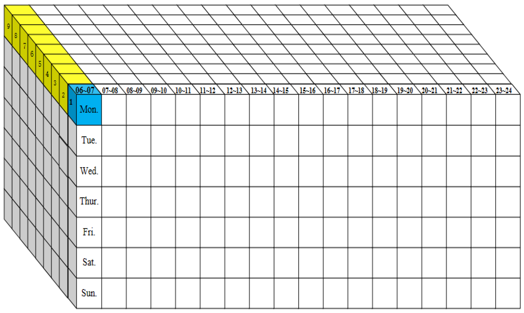
Since the GM (1,1) model has good prediction effect on the data with gentle variation, compared with the flat peak period, the passenger flow in the morning peak and the evening peak will increase. Compared with the passenger flow in the working day, the weekend passenger flow will decrease, so the daily passenger flow data does not vary gently. In order to reduce the impact of morning peak, evening peak and weekend passenger flow on the accuracy of the prediction model, a division of time segments in grid format of the subway station operation time was proposed to study the recent historical passenger flow of subway stations, and the hour-by-hour passenger flow GM (1,1) prediction model was established for different time periods.
Selecting the 9-week passenger flow data of a subway station in Chengdu as an example, the daily passenger transport time of the subway station from 06:00 to 24:00 was divided into 18 time periods with 1 h as the time interval. As shown in
Figure 1, each block could correspond to a specific time period. Among them, the blue block represented the corresponding passenger flow of the first Monday from 06:00 to 07:00, and the yellow block represented the corresponding passenger flow of every Monday from 06:00 to 07:00 for 9 weeks. They constituted a group of the original data of the GM (1,1) model. By analogy, the passenger flow prediction model corresponding to each time period was constructed. The hour-by-hour passenger flow GM (1,1) prediction model of 9 weeks could be obtained by integrating all the prediction values. Then, the hour-by-hour passenger flow and variation law in the future short-term (taking the 10th week as an example) could be predicted using the prediction model.
2.3. Establishment of Prediction Model
The GM (1,1) model represents a first-order linear dynamic model with a single variable. It is a first-order differential equation of single variable
x to time:
The passenger flow on the same day of the week during the same hour was used as the original data to build the GM (1,1) model. The predicted values were integrated to obtain the weekly hour-by-hour passenger flow variation law. Taking the passenger flow data of subway stations from 06:00 to 07:00 every Monday as an example, a passenger flow GM (1,1) model was established as follows:
For
X(0), the sequence
X(1) was generated by a one-time accumulation:
The prediction model was established for the first-order cumulatively generated sequence
X(1):
where
a, u are the parameters to be estimated, representing the development gray number and endogenous control gray number.
Expanding Formula (4) discretely, we can obtain:
Therefore,
a = −0.0129, u = 288.99,
X(0)(1) = 222, = −22,327.82,
X(0)(1) − = −22,549.82,
The passenger flow GM (1,1) model was as follows:
After analyzing the above results, we were able to draw the following conclusion:
By comparing the predicted passenger flow with the actual passenger flow, as shown in
Figure 2, it can be observed that the predicted value and the actual value have a good fit and consistent trend. This preliminary analysis suggests that the passenger flow GM (1,1) model can be utilized to predict variations in passenger flow during each period.
2.4. Model Checking
The test method of the gray prediction model is related to the joint degree test, residual test, and posterior difference test. Not all tests exhibit flawless accuracy, yet they generally fall within acceptable thresholds. In this paper, a posterior difference test method was used to test the passenger flow prediction model. The posterior difference ratio “C” was used to evaluate the model’s accuracy. Generally speaking, the smaller the value is, the better the model’s accuracy is. The accuracy levels of specific models are compared and presented in
Table 1. The following section outlines the step-by-step calculation process in detail.
The original sequence was:
The prediction sequence of gray model was:
The residual could be calculated as:
The mean and variance of X
(0)(k) were calculated as follows:
The mean and variance of
were calculated as follows:
and
are called the small error probability and posterior error ratio. The accuracy grade of the gray prediction is shown in
Table 1.
Table 1.
Gray prediction accuracy grade.
Table 1.
Gray prediction accuracy grade.
| p | C | Prediction Accuracy Level |
|---|
| ≥0.95 | <0.35 | Good |
| ≥0.80 | <0.50 | Qualified |
| ≥0.70 | <0.65 | Barely qualified |
| ≤0.70 | ≥0.65 | Unqualified |
According to the calculation results of the posterior error ratio (C = 0.24) and the small error probability (p = 1.00), it can be observed that the accuracy of the gray prediction model, specifically the GM (1,1) model, was evaluated using a grade table. The results indicated that the model exhibited good prediction accuracy, making it suitable for predicting the variation in passenger flow on an hourly basis at subway stations. By employing an analogy, the GM (1,1) model was developed to analyze the passenger flow for each period. This model allowed for the prediction of hourly passenger flow values at a subway station over the course of one week.
2.5. Prediction Results
Combing the actual passenger flow data of 9 weeks and the division way of time segments in grid format of the subway station operation time, the hour-by-hour passenger flow GM (1,1) prediction model was established, and 1134 predicted values were obtained by repeating the above prediction process. The variation law of hour-by-hour passenger flow over 9 weeks was obtained by sorting out the prediction results, as shown in
Figure 3. Since the GM (1,1) prediction model was essentially based on the exponential fitting of the least-squares method, the first point of the original sequence was eliminated, the actual value and the predicted value of the passenger flow shown in
Figure 3a were completely consistent.
As depicted in
Figure 3, the comparison between the 9-week passenger flow forecast and the actual passenger flow data revealed a minimal overall error. This finding highlights the advantage of using the GM (1,1) model, as it is capable of accurately predicting passenger flow even in cases where the data exhibit gradual changes. The average relative error evaluation index was employed to compute the error magnitude of the entire forecasting procedure. As indicated in
Table 2, the analysis revealed that the average relative error (a) for the 9-week hourly passenger flow prediction results was 5.67%. The maximum relative error observed was 15%, and all relative errors fell within the acceptable range of 20%. Therefore, it can be concluded that the prediction errors meet the specified requirements.
If the relative error of the passenger flow GM (1,1) prediction model was less than 20%, this indicated that it met the requirements, and if it was less than 10%, this indicated that it met the higher requirements. The results show that the subway stations that use the grid format to segment operation time and passenger flow have a relatively small error at 1 h interval, which can be avoided by limiting the general (1, 1) model to only apply to the data with mild changes.
Based on the established 9-week hour-by-hour passenger flow GM (1,1) prediction model, the future short-term passenger flow (taking the 10th week as an example) was predicted, and the prediction results of the 10th week were compared with the actual passenger flow. As shown in
Figure 4, it could be seen that the predicted value and the actual value were well fitted. The maximum relative error was 14.97%, less than 20%, indicating that the improved passenger flow GM (1,1) prediction model was relatively accurate and could be used to predict the future short-term passenger flow of subway stations. Overall, it reduced the prediction error caused by the large fluctuation of passenger flow, effectively avoided the limits of the GM (1,1) model, and further provided theoretical support for the study of dynamic load of air-conditioning system in subway stations.
3. Dynamic Load Variation Law
A subway ventilation and air-conditioning system includes a tunnel ventilation system, public area ventilation and air-conditioning system (large air conditioning), and equipment management room ventilation and air-conditioning system (small system). This paper took an air-conditioning system in a public area as the research object and studied the dynamic load variation caused by the variation of hour-by-hour passenger flow.
This paper takes the air-conditioning system in the public area of a subway station in Chengdu as the research object to explore the dynamic load change rule caused by hourly passenger flow change, mainly including the station hall and platform, to provide passengers with a comfortable and hygienic transitional environment in the passenger activity area. The dimensions of the station hall are 180.6 m × 20.6 m × 3 m, with a working area temperature of tn = 29 °C, supply air temperature difference of 10 °C, supply air temperature to = 19 °C; platform: 140 m × 10 m × 3 m, working area temperature tn = 27 °C, supply air temperature difference of 8 °C, and supply air temperature to = 19 °C.
According to the study, the subway station in the screen door system mode could be regarded as a relatively closed underground box-shaped building. In general, the cooling load of subway station environmental control system Q
l included lighting load Q
z, equipment load Q
s, envelope heat transfer load Q
w, personnel load Q
p, fresh air load Q
x, and air infiltration load Q
t caused by the entrance/exit infiltration wind. Among them, the personnel load would fluctuate greatly with the variation of passenger flow, and the fresh air load would be affected by the outdoor air enthalpy value, which belonged to the dynamic load. Therefore, from the perspective of reducing operation energy consumption and cost saving, the hour-by-hour calculation parameters of outdoor air could be calculated according to the variation law of short-term passenger flow in the future, and the dynamic load distribution could be obtained by summarizing various sub-loads [
25]. The air supply parameters of the air-conditioning system of the subway station could be adjusted in time to alleviate the energy waste caused by the operation of the subway station to a certain extent.
3.1. Calculation Method of Each Sub-Load
- (1)
Lighting load Qz: This value was calculated in accordance with the unit area index of 20 W/m2. According to the actual size model of the subway station, the station hall length was 140 m, the width was 20.6 m, the area was 2884 m2, and station platform length was 180.6 m, the width was 10 m (passenger holding area between the screen doors on both sides), and the area was 1806 m2.
- (2)
Equipment load Qs: The total equipment load of the subway station was calculated according to the heat dissipation of single equipment and the number of each equipment in public area.
- (3)
Envelope load Qw: At present, most subway stations are equipped with screen door systems; therefore, the proportion of the envelope load to the ventilation and air-conditioning load of the subway station was relatively small and could basically be ignored.
- (4)
Entrance/exit air infiltration load Q
t: The area index was used for estimation. the area thermal index of entrance/exit infiltration heat exchange was 200 W/m
2 [
26], the area of the entrance/exit could determine the infiltration heat exchange of the entrance. The subway station had four entrances; the width and height of each entrance was 6.5 m × 2.5 m. In addition, when the screen door was opened, part of the load was released to the platform, which could be estimated at 10 kW/side [
27].
- (5)
Personnel load Qp: According to the hour-by-hour entering and leaving passenger flow and the time passengers stayed in the public area, the simultaneous passenger flow in the station was calculated, and the hour-by-hour personnel load in the station hall and platform was further calculated by combining with the total heat dissipation of passengers. One of the special features of the personnel load in subway stations is the short detention time of passengers, and the behavior of passengers in stations can be characterized by “short stay”.
The relationship among the number of subway stations at the same time in an hour and the number of passengers entering and leaving the station and the residence time was calculated as follows using Equations (14) and (15) [
28].
where
Nc—number of people in the station hall at the same time, people;
Np—number of people in the station platform at the same time, people;
A1—number of people entering the station hour by hour, people/h;
A2—number of people leaving the station hour by hour, people/h;
a1—time for passengers to enter the station and stay in the station hall, taking 2 min;
a2—time for passengers to enter the station and stay in the station platform, taking 2 min;
b1—time for passengers to leave the station and staying in the station hall, taking 1.5 min;
b2—time for passengers to leave the station and staying in the station platform, taking 1.5 min;
Qc—station hall personnel load, kW;
Qp—station platform personnel load, kW;
qc—total heat dissipation of station hall passengers, taking 183 W/person;
qp—total heat dissipation of station platform passengers, taking 181 W/person;
Wc—station hall personnel wet load, kg/h;
Wp—station platform personnel wet load, kg/h;
dc—the amount of moisture dissipation per passenger in the station hall, taking 212 g/(h-people);
dp—the amount of moisture dissipation per passenger in the station platform, taking 203 g/(h-people).
3.2. Calculation Results of Each Cooling Load
The calculation results of lighting load, equipment load, and entrance/exit infiltration load, as well as the hourly personnel load calculated according to the synchronous passenger flow of subway stations, are shown in
Table 3.
3.3. Air Supply Volume of the Air-Conditioning System
According to the calculated cooling load value of the station hall and station platform and the primary return air treatment process of the large subway station system, the hourly air supply and fresh air volume were calculated. The air treatment process is shown in
Figure 5. ‘W’ was the outdoor air state point. ‘N
1’ and ‘N
2’ were the air state points in the station hall and station platform. Respectively, the return air from the station hall and station platform was mixed to state point ‘N’, which was mixed with outdoor state point ‘W’ to state point ‘C’ after cooling and dehumidifying to air dew point ‘L’ with a relative humidity of 95; then, equal wet heating to the air supply state point ‘O’ occurred.
The Subway Design Code stipulates that when an air-conditioning system is used in the subway station, the calculated air temperature in the station hall should be 2 °C~3 °C below the calculated outdoor air dry bulb temperature and below 30 °C. The calculated air temperature in the station platform should be 1~2 °C below the calculated temperature in the station hall, and the relative humidity should be controlled at 40~70%. According to the design requirements, the dry bulb temperature of the station hall N1 was 29 °C, and the relative humidity was 51.9%. The dry bulb temperature of the station platform N2 was 27 °C, and the relative humidity was 57.6%. The enthalpy value of each state point could be obtained by checking the enthalpy and humidity diagram. The temperature difference of air supply to the station hall was 10 °C, and the temperature difference of air supply to the station platform was 8 °C, that was, the air supply state point O was 19 °C.
The air supply volume of station hall and platform hour-by-hour were calculated according to Formula (20), and the calculation results are shown in
Figure 6.
where:
V—air supply volume of the air-conditioning system, m3/h;
Q—air-conditioning system cooling load, kW;
—enthalpy of the indoor state point, kJ/kg;
—enthalpy of the air supply point, kJ/kg;
Figure 6.
Summary of the hour-by-hour air supply to the station hall and platform.
Figure 6.
Summary of the hour-by-hour air supply to the station hall and platform.
3.4. Air-Conditioning System Fresh Air Volume and Fresh Air Load Calculation
The fresh air volume of the air-conditioning season in public areas of subway stations was taken as the greater of the following two values [
29]:
- (1)
According to the Health Code for Centralized Air Conditioning Ventilation Systems in Public Places (WS 3942012), the fresh air volume for personnel in public areas of stations was unified at 20 m3/h/person for the whole line.
- (2)
The fresh air volume was not less than 10% of the total air supply volume of the system.
The fresh air load was derived from the outdoor air-conditioning hour-by-hour parameters in the summer. The outdoor air calculation parameters in the summer of Chengdu are shown in
Table 4, and the outdoor hour-by-hour air parameters in the summer were calculated according to Formulas (21), (23), and (27).
- (1)
Outdoor air hour-by-hour dry bulb temperature
—outdoor calculated hour-by-hour temperature, °C;
—calculated average daily temperature outside the air conditioner in summer, °C;
—the hour-by-hour coefficient of variation of outdoor temperature, as shown in
Table 5;
—the average daily difference was calculated outdoors in summer, °C;
—summer air conditioning outdoor calculated dry bulb temperature, °C;
Table 5.
Hour-by-hour variation coefficients of outdoor temperature.
Table 5.
Hour-by-hour variation coefficients of outdoor temperature.
| Time | 1 | 2 | 3 | 4 | 5 | 6 |
|---|
| β | −0.35 | −0.38 | −0.42 | −0.45 | −0.47 | −0.41 |
| time | 7 | 8 | 9 | 10 | 11 | 12 |
| β | −0.28 | −0.12 | 0.03 | 0.16 | 0.29 | 0.40 |
| time | 13 | 14 | 15 | 16 | 17 | 18 |
| β | 0.48 | 0.52 | 0.51 | 0.43 | 0.39 | 0.28 |
| time | 19 | 20 | 21 | 22 | 23 | 24 |
| β | 0.14 | 0.00 | −0.10 | −0.17 | −0.23 | −0.26 |
- (2)
Outdoor air hour-by-hour wet bulb temperature
—outdoor air wet bulb temperature in summertime, °C;
ts—calculated outdoor wet bulb temperature for air conditioning in summer, °C;
—standard atmospheric pressure, 101.325 kPa;
B′—local atmospheric pressure in summer, 94.8 kPa;
tw—calculated outdoor dry bulb temperature for air conditioning in summer, °C;
tp—average daily temperature of air conditioning in summer, °C;
—calculate the moments, taking 6, 7, 8, ……,24;
—constants;
—correction factor, taking 5.
- (3)
Humidity content of outdoor air hour-by-hour
The saturated moisture content of outdoor air was a single-valued function of the wet bulb temperature and could be expressed as:
where
—the saturated air moisture content per unit mass of dry air at the moment of time, g/kg.
- (4)
Timely hour-by-hour enthalpy of outdoor air
The enthalpy of outdoor air at any given moment was a single-valued function of its corresponding wet bulb temperature, according to the defining equation for the enthalpy of air:
Organizing Equations (24)–(26) yields:
where
h—enthalpy of air, kJ/kg;
t—air dry bulb temperature, °C;
d—air moisture content per unit mass of dry air, g/kg;
—enthalpy of outdoor air at the moment of calculation, hour-by-hour calculation of enthalpy, kJ/kg.
- (5)
Calculation results of outdoor air hour-by-hour parameters
Based on the above equations for the outdoor air state parameters in the summer, the results of the hour-by-hour calculations of outdoor air parameters in Chengdu in the summer are shown in
Figure 7.
- (6)
Fresh air load Qx
The fresh air load was calculated according to Equation (28), and the results of the calculation of the fresh air volume and fresh air load of the station hall and platform hour-by-hour are shown in
Figure 8.
where
Qx—fresh air load, W;
ρ—fresh air density, 1.2 kg/m3;
Vx—fresh air volume, 20 m3/(h·person);
—outdoor air enthalpy, kJ/kg;
—indoor air enthalpy, kJ/kg.
Figure 8.
Summary of the hour-by-hour fresh air volume and fresh air load of the station hall and platform.
Figure 8.
Summary of the hour-by-hour fresh air volume and fresh air load of the station hall and platform.
3.5. Summary of Hour-by-Hour Load Calculation Results
Based on the calculated individual load results, the summary could be derived from the weekday hour-by-hour load, as shown in
Figure 9, and the weekend hour-by-hour load, as shown in
Figure 10, by the same method.
3.6. Energy Saving Analysis
The comparative graphs of each sub-load and constant working load on working days and weekends are shown in
Figure 11 and
Figure 12, respectively.
As could be seen from
Figure 11 and
Figure 12, the total load for a weekday day was 6682.05 kW; the dynamic load was 5212.28 kW, a total reduction of 1469.77 kW, or 22.00%, when the fixed operating load was calculated to meet the peak passenger load requirements. The total load on a weekend day was 5489.21 kW; the dynamic load was 4880.63 kW, a total reduction of 608.58 kW, or 11.09%. In contrast, the hour-by-hour passenger flow on weekdays fluctuated more. After predicting the hour-by-hour passenger flow law, the operation strategy of the air-conditioning system was adjusted according to the dynamic load in time, and the reduction of air conditioning operation load on weekdays was larger than that on weekends.
In summary, compared with the operation of the air-conditioning system under fixed working conditions, the dynamic load calculated according to the hour-by-hour passenger flow law had a significant reduction. It could be used to guide the operation and management of the air-conditioning system in subway stations and further provide reference significance for the optimization of the energy-saving of the air-conditioning system in subway stations.


