

Analysis of Thin Carbon Reinforced Concrete Structures through Microtomography and Machine Learning


Abstract
:1. Introduction
2. Materials and Methods
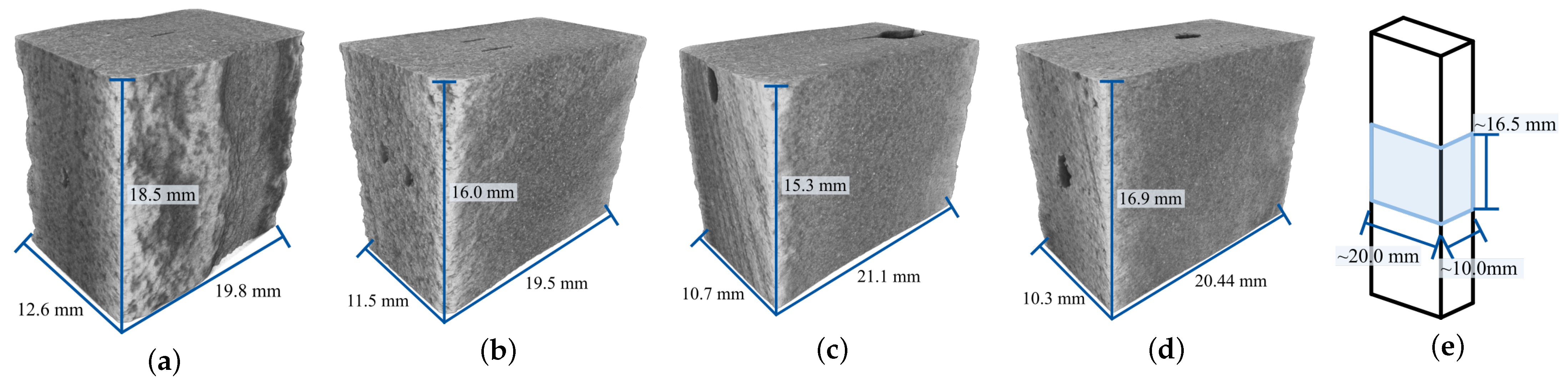
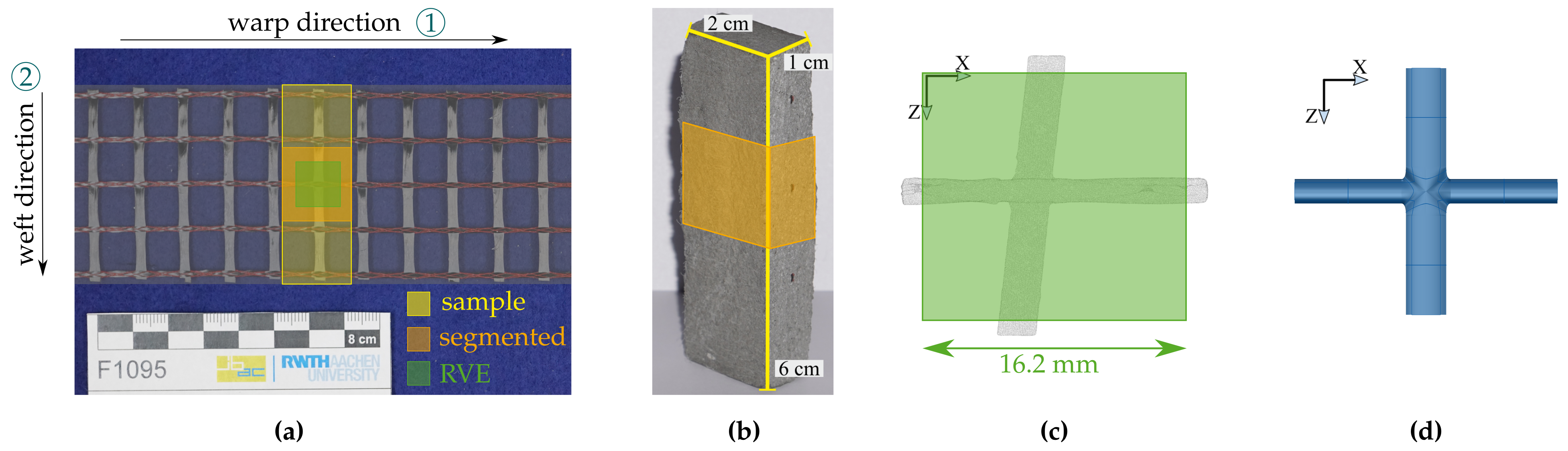
2.1. Specimens
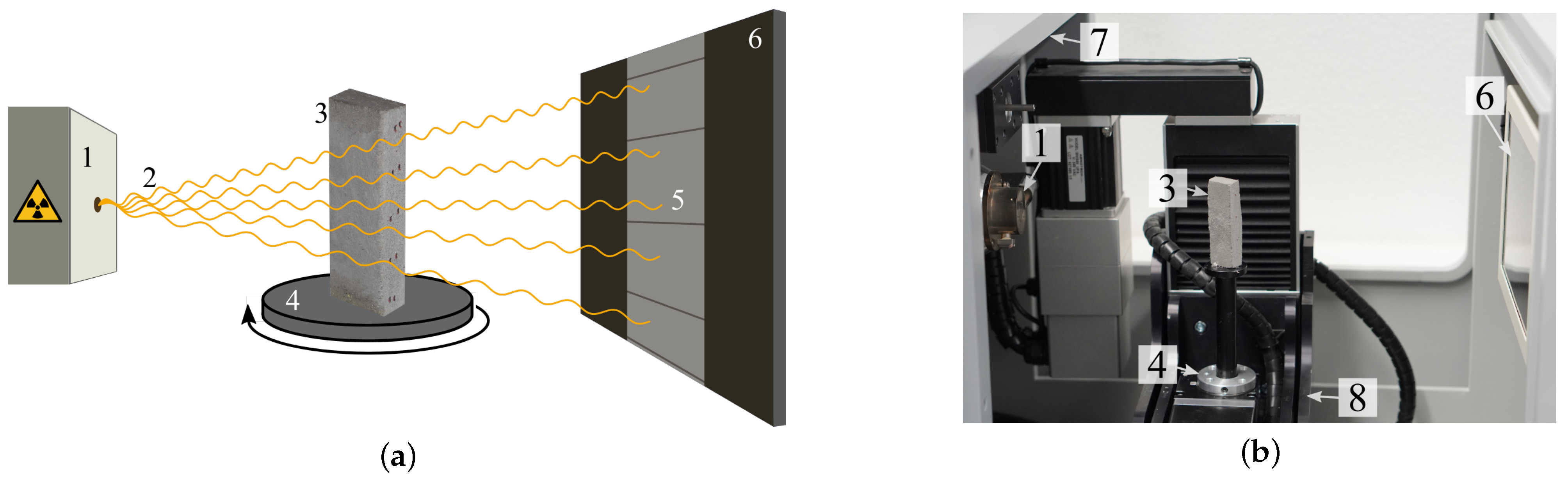
2.2. Microtomography
2.3. AI-Based Segmentation
2.3.1. Training Data
2.3.2. Augmentation
2.3.3. Training and Metrics
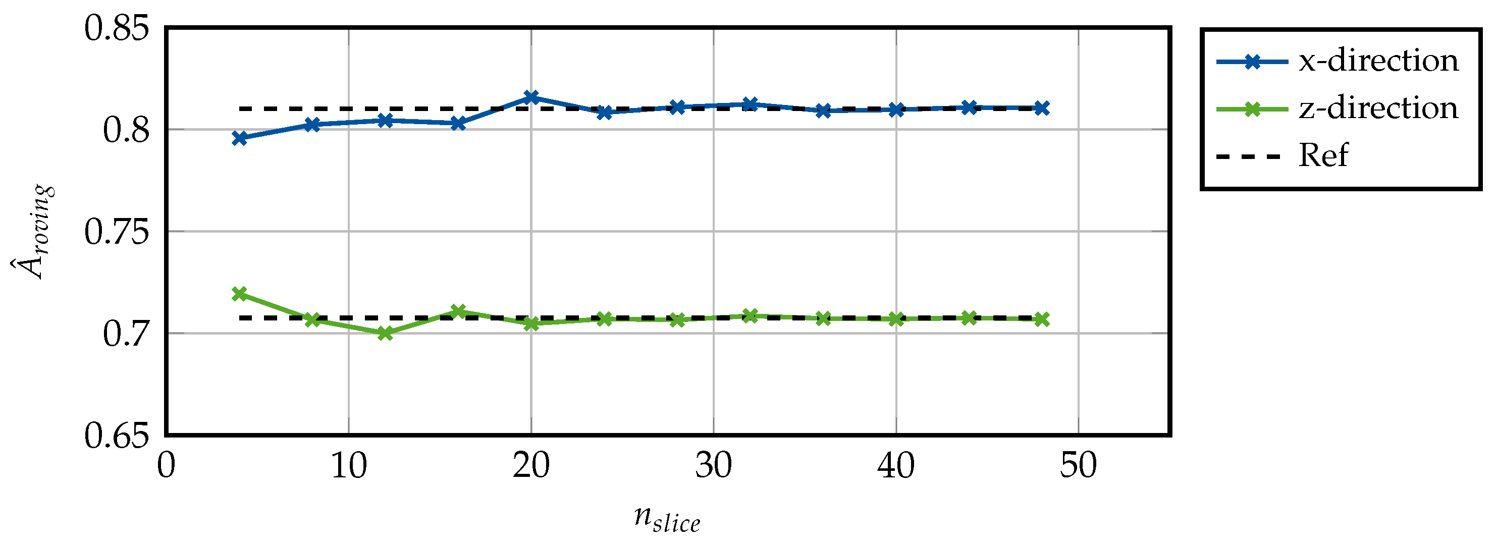
2.4. Roving Extraction
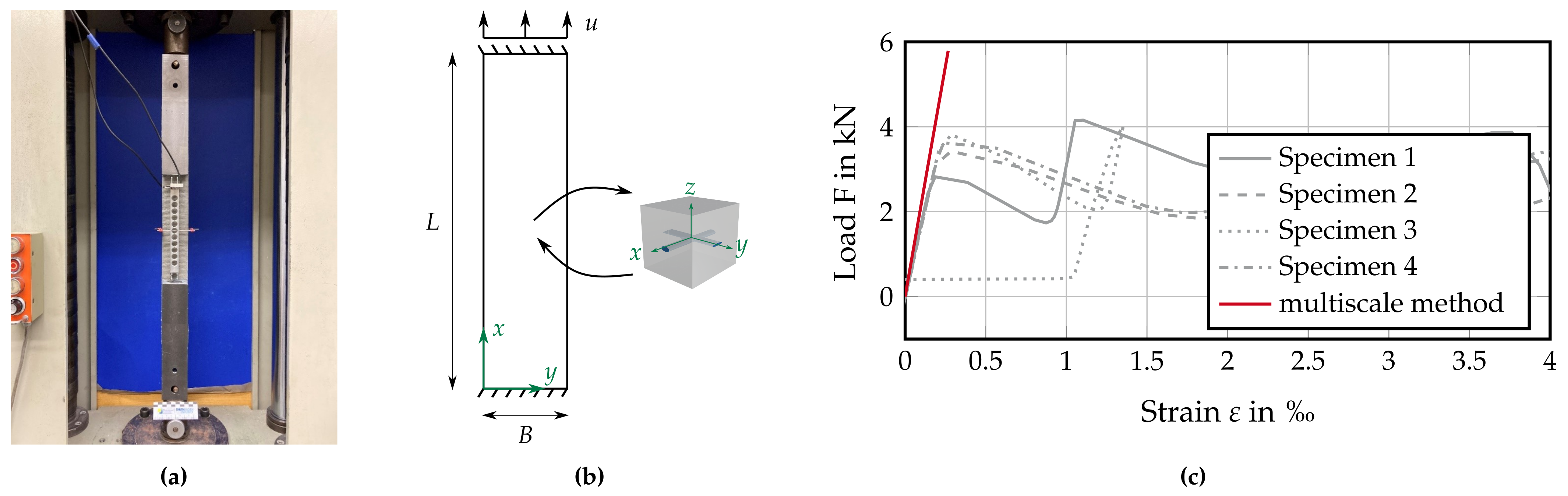
2.5. Multiscale Modeling
2.6. Scaled Boundary Isogeometric Analysis
2.7. Parameterized RVE and Definition of Characteristic Geometric Properties
2.7.1. Roving Dimensions and
2.7.2. In-Plane Dimensions
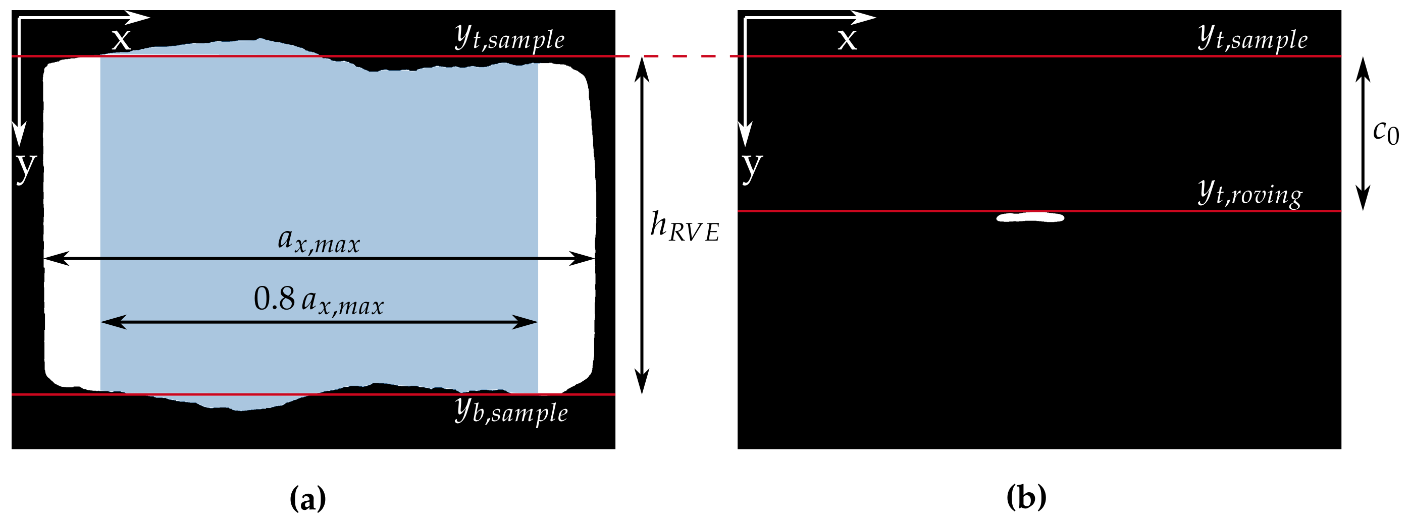
2.7.3. Shell Thickness
2.7.4. Concrete Cover
2.7.5. Concluding Assumptions
- Rovings are orthogonal to each other.
- Only one intersection of rovings is considered.
- Rovings are approximated as elliptical cylinders.
3. Results and Discussion
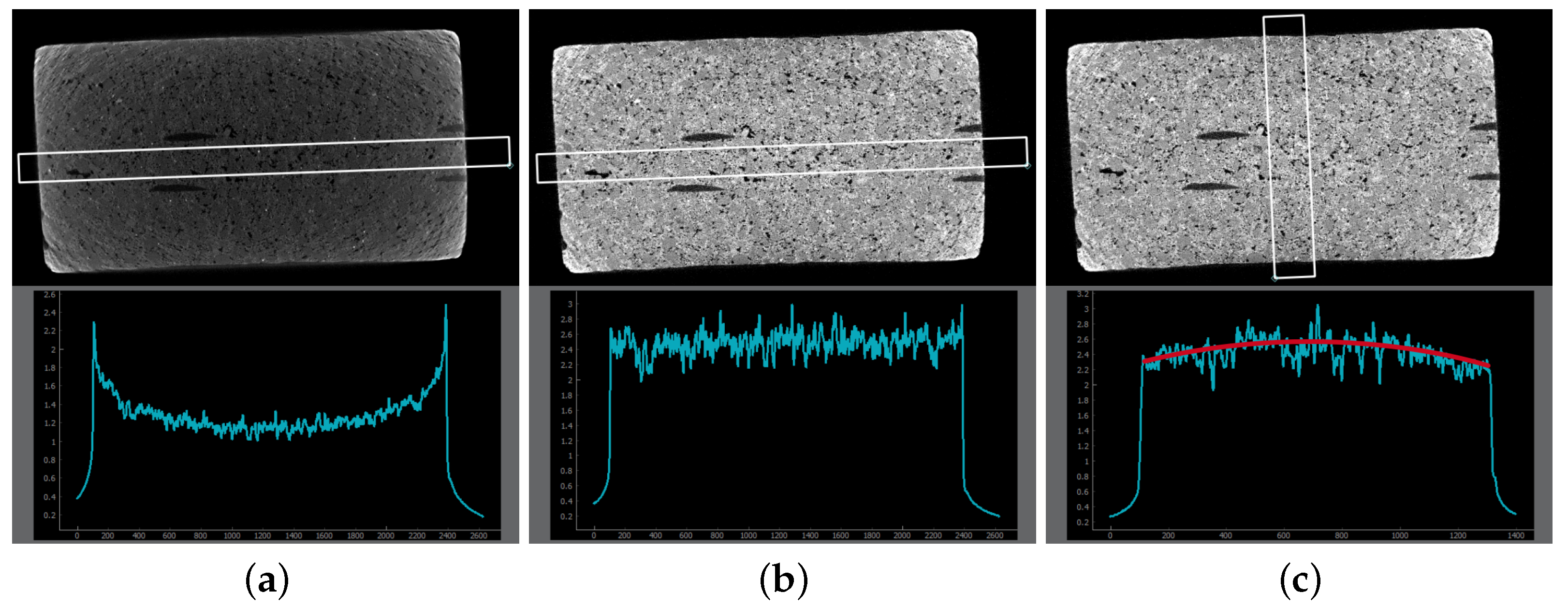
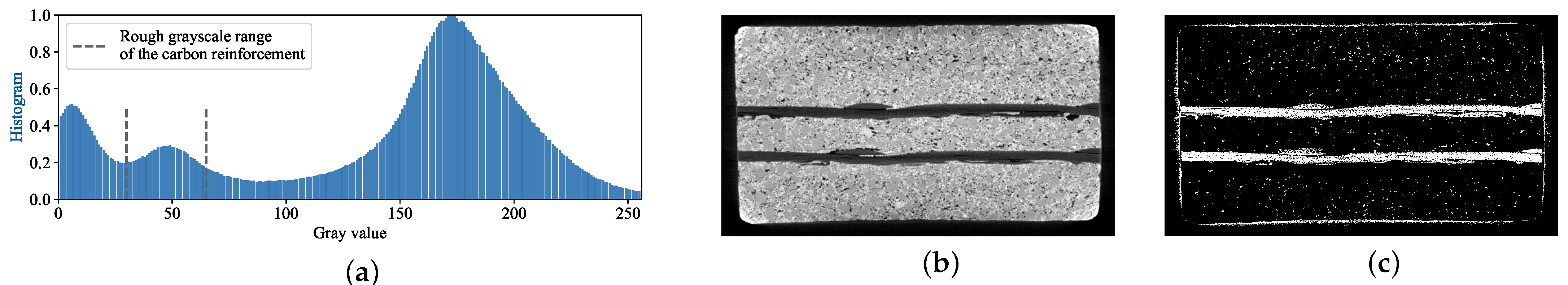
3.1. Microtomography
3.2. Deep Learning
- Weak offline augmentation:
- –
- Rotation around X, Y, and Z;
- Strong offline augmentation:
- –
- Rotation (around X, Y, and Z), resizing, flipping, tilting, squeezing, noise addition, blurring, sharpening, contrast manipulation, brightness manipulation;
- Online augmentation:
- –
- Offline: rotation around X and Y due to the difference in input height (128), width (128) and depth (64);
- –
- Online: rotation (around Z), resizing, flipping, tilting, squeezing, noise addition, blurring, sharpening, contrast manipulation, brightness manipulation.
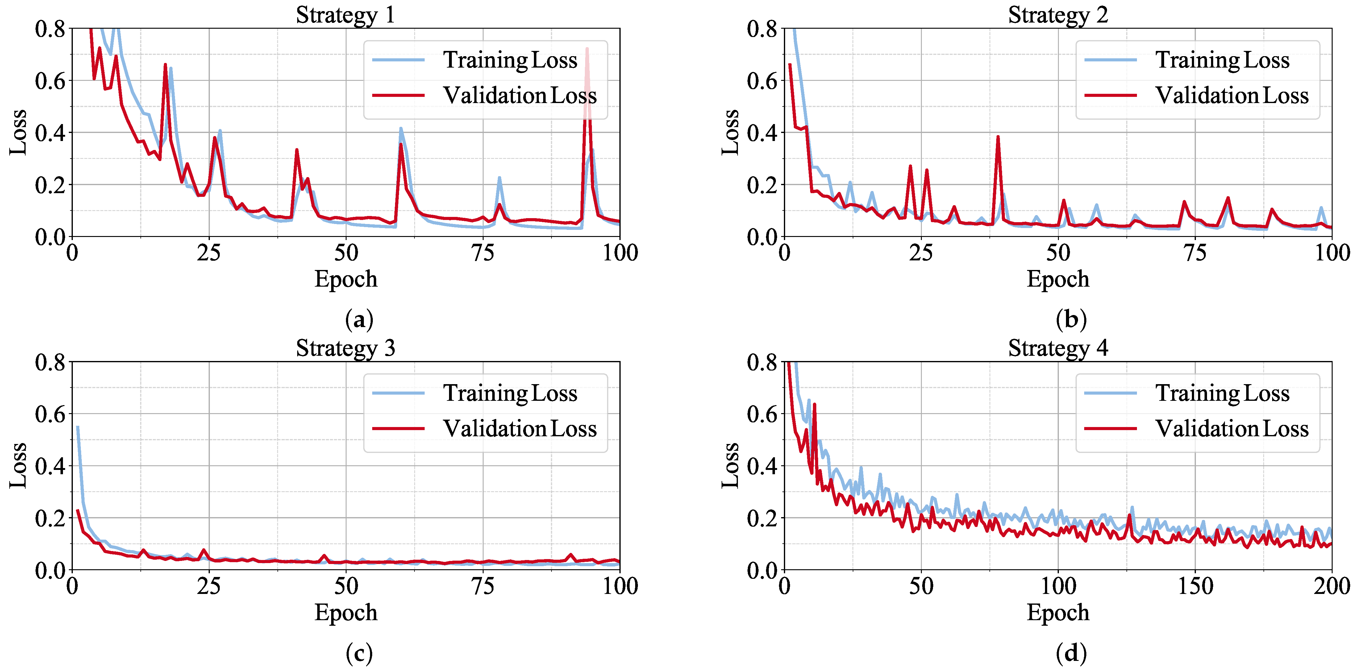
3.2.1. Hardware and Training Duration
3.2.2. Training Results
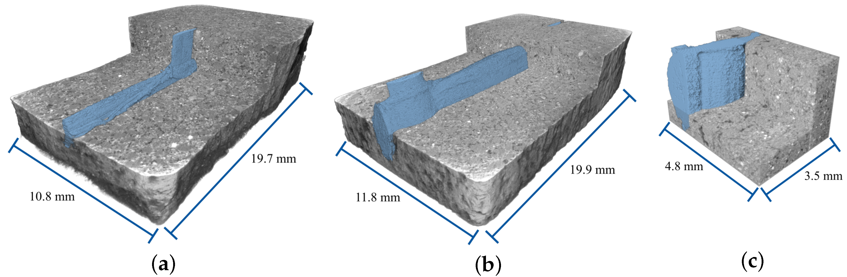
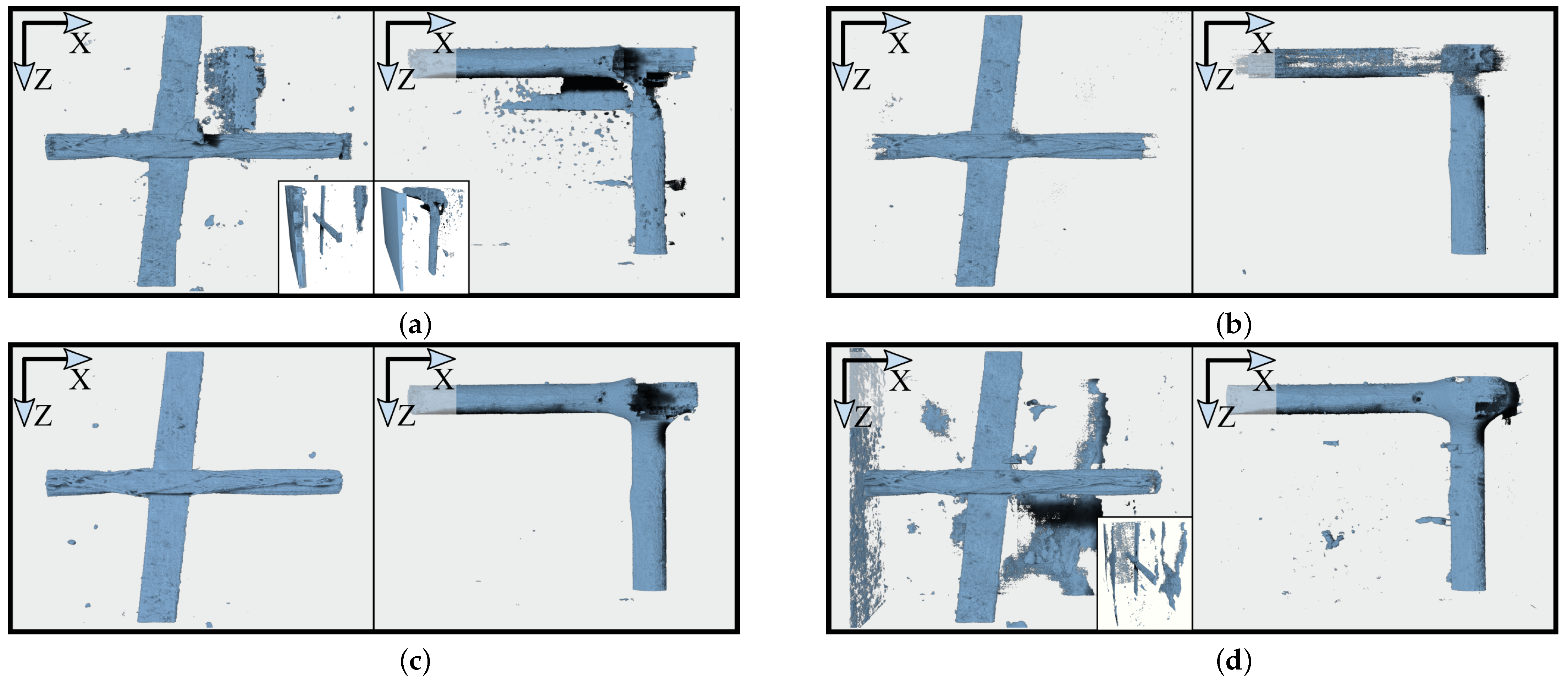
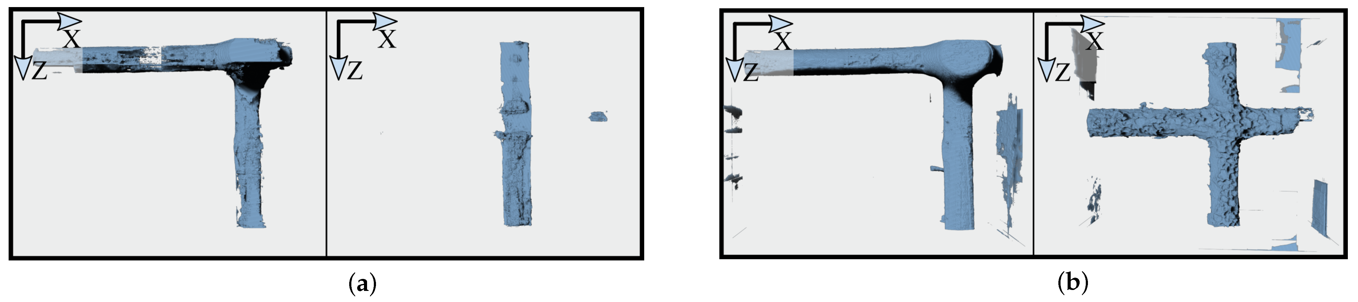
3.3. Roving Extraction
3.4. Parameterized RVE and Definition of Characteristic Geometric Properties
3.4.1. Roving Dimensions and
3.4.2. In-Plane Dimensions
3.4.3. Shell Thickness
3.4.4. Concrete Cover
3.4.5. Example
3.4.6. Assumptions
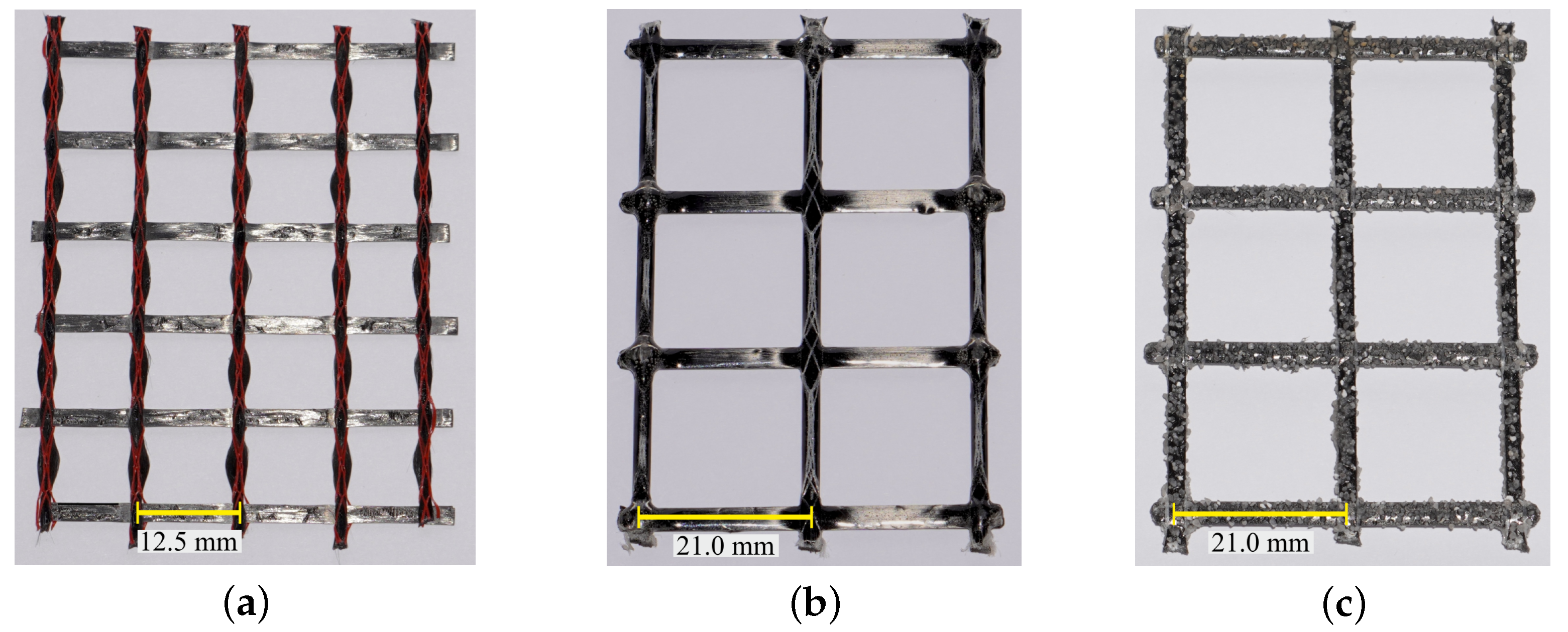
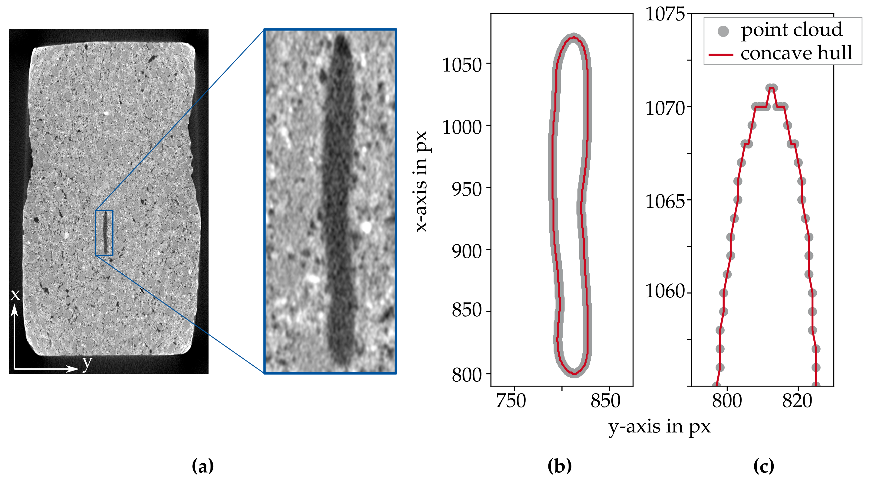
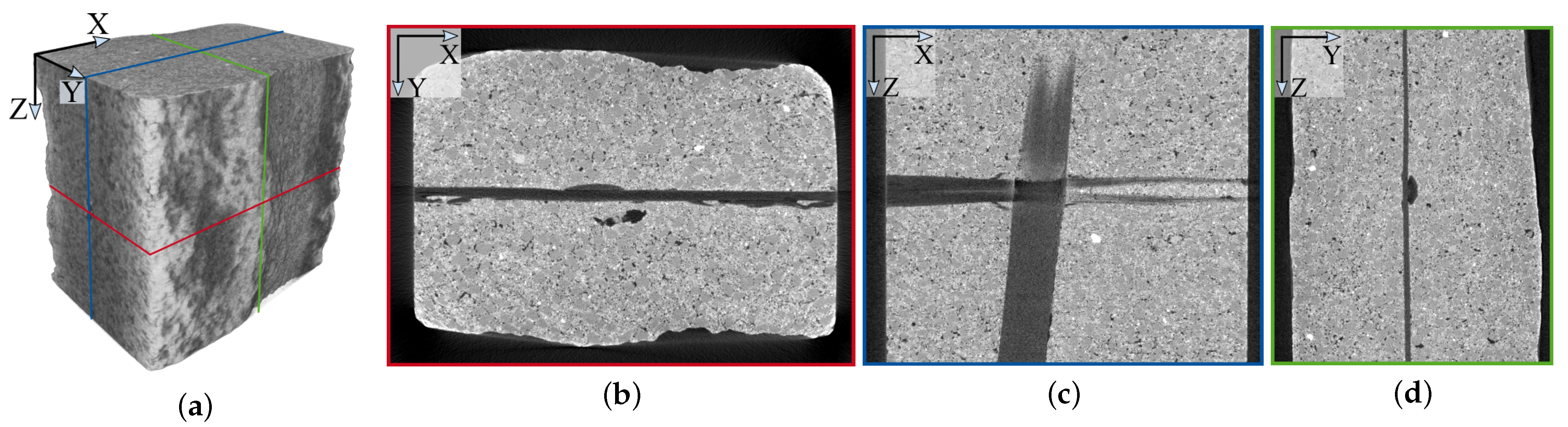
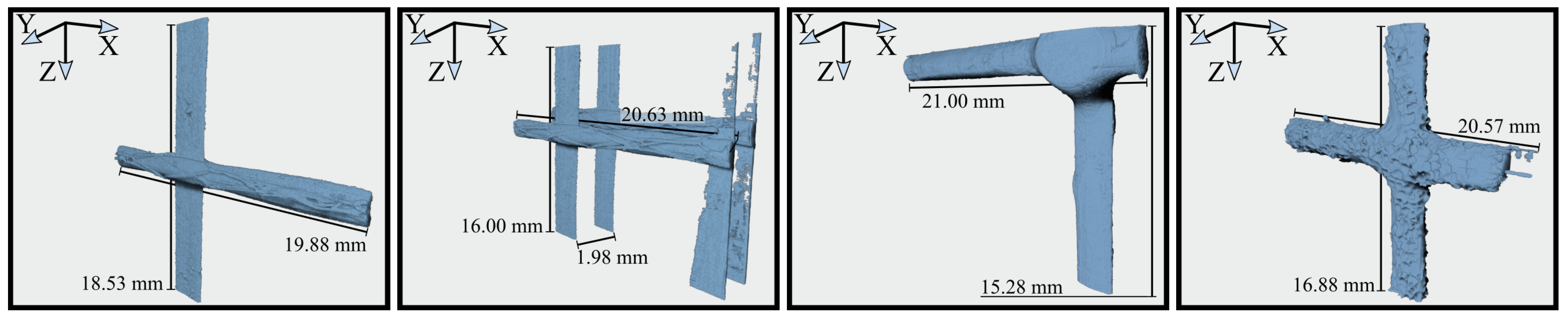
- Orthogonality: From Figure 2c, it is clear that the rovings in warp and weft directions were not perfectly orthogonal to each other. However, the rotation of the extracted roving led to only small deviations in the derived geometric properties. Additionally, the distortion was introduced by the extrusion process. Using classical production methods, the distortion of the textile is less distinct. Thus, the assumption of orthogonal rovings is valid.
- A single roving intersection is sufficient for the RVE. This assumption is valid as long as manufacturing errors, which could lead to varying shell thicknesses or concrete covers, can be excluded. Ideally, the segmented area is greater than or equal to the RVE size in order to properly approximate the roving dimensions.
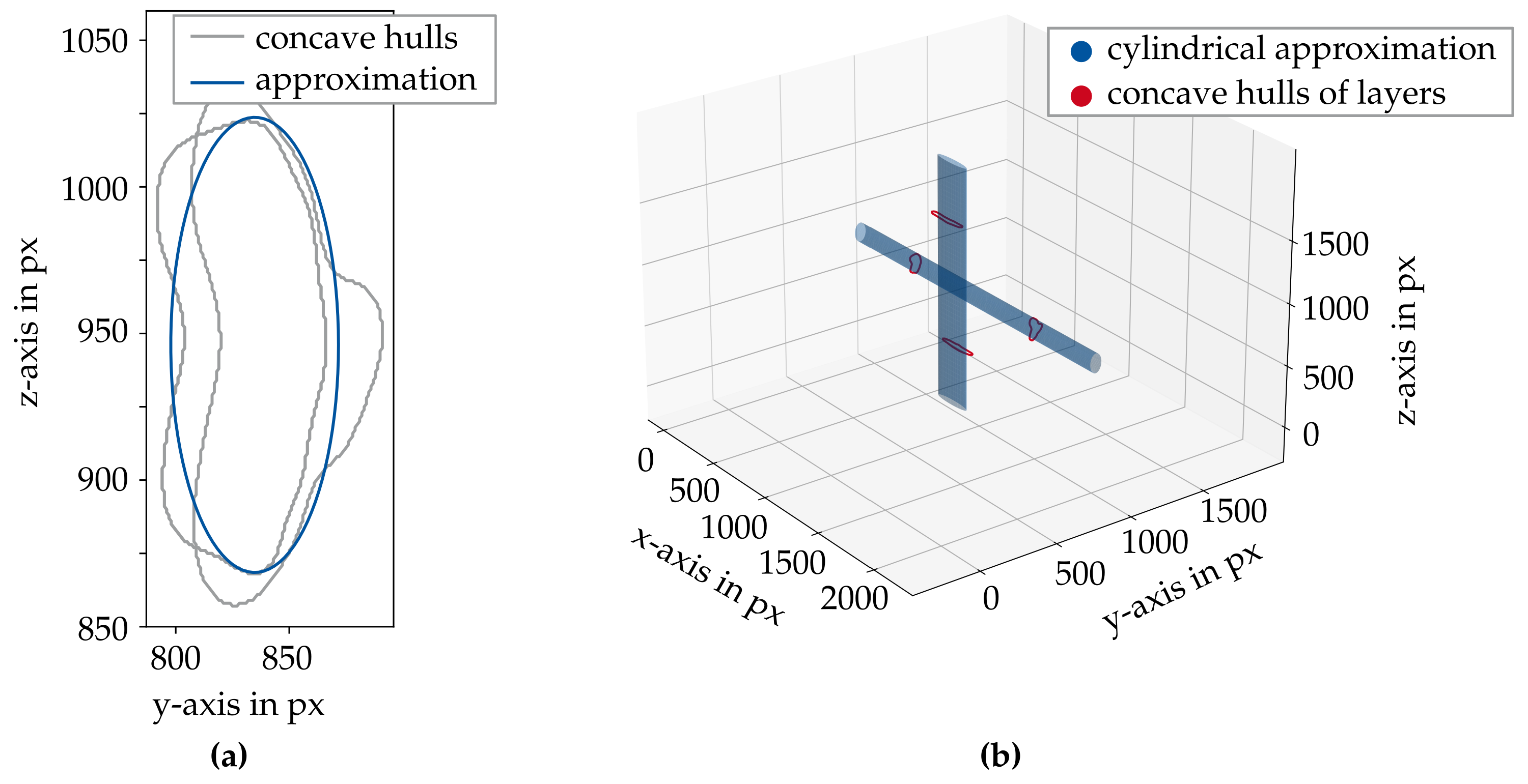
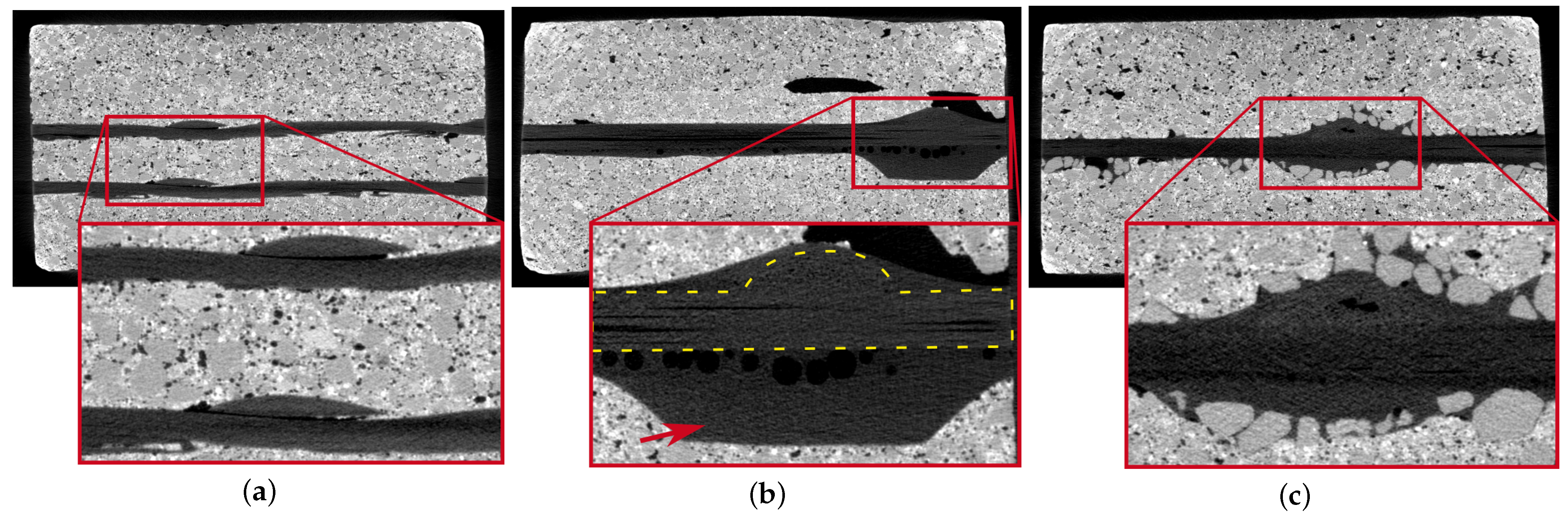
- Elliptical cross-sections are assumed for both rovings. Analysis of the cross-sectional images revealed that small height-to-width ratios should be considered for the roving. In the context of the presented linear-elastic tensile test, the shape approximation proved to be satisfactory.
4. Conclusions
Author Contributions
Funding
Data Availability Statement
Acknowledgments
Conflicts of Interest
Abbreviations
| CNN | Convolutional neural network |
| CRC | Carbon reinforced concrete |
| CT | Computed tomography |
| LabMorTex | Laboratory Mortar Extruder |
| NURBS | Non-uniform rational B-splines |
| RVE | Representative volume element |
| SBIGA | Scaled boundary isogeometric analysis |
References
- Scheerer, S.; Zobel, R.; Müller, E.; Senckpiel-Peters, T.; Schmidt, A.; Curbach, M. Flexural Strengthening of RC Structures with TRC—Experimental Observations, Design Approach and Application. Appl. Sci. 2019, 9, 1322. [Google Scholar] [CrossRef]
- Beckmann, B.; Bielak, J.; Bosbach, S.; Scheerer, S.; Schmidt, C.; Hegger, J.; Curbach, M. Collaborative research on carbon reinforced concrete structures in the CRC/TRR 280 project. Civ. Eng. Des. 2021, 3, 99–109. [Google Scholar] [CrossRef]
- Bielak, J.; Kollegger, J.; Hegger, J. Shear in Slabs with Non-Metallic Reinforcement. Ph.D. Thesis, Lehrstuhl und Institut für Massivbau, RWTH Aachen University, Aachen, Germany, 2021. [Google Scholar] [CrossRef]
- Morales Cruz, C. Supplementary Data to Crack-distributing Carbon Textile Reinforced Concrete Protection Layers. Ph.D. Thesis, Lehrstuhl für Baustoffkunde–Bauwerkserhaltung, RWTH Aachen University, Aachen, Germany, 2022. [Google Scholar] [CrossRef]
- Kalthoff, M.; Raupach, M.; Matschei, T. Investigation into the Integration of Impregnated Glass and Carbon Textiles in a Laboratory Mortar Extruder (LabMorTex). Materials 2021, 14, 7406. [Google Scholar] [CrossRef]
- Kalthoff, M.; Raupach, M.; Matschei, T. Extrusion and Subsequent Transformation of Textile-Reinforced Mortar Components—Requirements on the Textile, Mortar and Process Parameters with a Laboratory Mortar Extruder (LabMorTex). Buildings 2022, 12, 726. [Google Scholar] [CrossRef]
- Kalthoff, M.; Bosbach, S.; Backes, J.G.; Morales Cruz, C.; Claßen, M.; Traverso, M.; Raupach, M.; Matschei, T. Fabrication of lightweight, carbon textile reinforced concrete components with internally nested lattice structure using 2-layer extrusion by LabMorTex. Constr. Build. Mater. 2023, 395, 132334. [Google Scholar] [CrossRef]
- Mester, L.; Wagner, F.; Liebold, F.; Klarmann, S.; Maas, H.G.; Klinkel, S. Image-Based Modelling and Analysis of Carbon-Fibre Reinforced Concrete Shell Structures. In Proceedings of the Concrete Innovation for Sustainability, Oslo, Norway, 12–16 June 2022; Volume 6, pp. 1631–1640. [Google Scholar]
- Scholzen, A.; Chudoba, R.; Hegger, J. Dünnwandiges Schalentragwerk aus textilbewehrtem Beton. Beton- Und Stahlbetonbau 2012, 107, 767–776. [Google Scholar] [CrossRef]
- Wagner, F.; Eltner, A.; Maas, H.G. River water segmentation in surveillance camera images: A comparative study of offline and online augmentation using 32 CNNs. Int. J. Appl. Earth Obs. Geoinf. 2023, 119, 103305. [Google Scholar] [CrossRef]
- Wagner, F. Carbon Rovings Segmentation Dataset. 2023. Available online: https://www.kaggle.com/datasets/franzwagner/carbon-rovings (accessed on 22 August 2023).
- Berger, M.; Tagliasacchi, A.; Seversky, L.M.; Alliez, P.; Guennebaud, G.; Levine, J.A.; Sharf, A.; Silva, C.T. A Survey of Surface Reconstruction from Point Clouds. Comput. Graph. Forum 2017, 36, 301–329. [Google Scholar] [CrossRef]
- Huang, Z.; Wen, Y.; Wang, Z.; Ren, J.; Jia, K. Surface Reconstruction from Point Clouds: A Survey and a Benchmark. arXiv 2022, arXiv:2205.02413. [Google Scholar] [CrossRef]
- Vukicevic, A.M.; Çimen, S.; Jagic, N.; Jovicic, G.; Frangi, A.F.; Filipovic, N. Three-dimensional reconstruction and NURBS-based structured meshing of coronary arteries from the conventional X-ray angiography projection images. Sci. Rep. 2018, 8, 1711. [Google Scholar] [CrossRef]
- Wang, Y.; Gao, L.; Qu, J.; Xia, Z.; Deng, X. Isogeometric analysis based on geometric reconstruction models. Front. Mech. Eng. 2021, 16, 782–797. [Google Scholar] [CrossRef]
- Grove, O.; Rajab, K.; Piegl, L.A. From CT to NURBS: Contour Fitting with B-spline Curves. Comput.-Aided Des. Appl. 2010, 7, 1–19. [Google Scholar] [CrossRef]
- Chasapi, M.; Mester, L.; Simeon, B.; Klinkel, S. Isogeometric analysis of 3D solids in boundary representation for problems in nonlinear solid mechanics and structural dynamics. Int. J. Numer. Methods Eng. 2021. [Google Scholar] [CrossRef]
- Hughes, T.J.R.; Cottrell, J.A.; Bazilevs, Y. Isogeometric analysis: CAD, finite elements, NURBS, exact geometry and mesh refinement. Comput. Methods Appl. Mech. Eng. 2005, 194, 4135–4195. [Google Scholar] [CrossRef]
- Cottrell, J.A.; Hughes, T.J.R.; Bazilevs, Y. Isogeometric Analysis: Toward Integration of CAD and FEA; John Wiley and Sons: Hoboken, NJ, USA, 2009. [Google Scholar]
- ProCon X-Ray GmbH. PXR PROCON X-RAY. 2020. Available online: https://procon-x-ray.de/ct-xpress/ (accessed on 17 September 2023).
- Millner, M.R.; Payne, W.H.; Waggener, R.G.; McDavid, W.D.; Dennis, M.J.; Sank, V.J. Determination of effective energies in CT calibration. Med Phys. 1978, 5, 543–545. [Google Scholar] [CrossRef]
- Tan, Y.; Kiekens, K.; Welkenhuyzen, F.; Kruth, J.; Dewulf, W. Beam hardening correction and its influence on the measurement accuracy and repeatability for CT dimensional metrology applications. In Proceedings of the 4th Conference on Industrial Computed Tomography (iCT), Wels, Austria, 19–21 September 2012; Volume 17, pp. 355–362. [Google Scholar]
- Ciresan, D.; Giusti, A.; Gambardella, L.; Schmidhuber, J. Deep Neural Networks Segment Neuronal Membranes in Electron Microscopy Images. Adv. Neural Inf. Processing Syst. 2012, 25, 1–9. Available online: https://papers.nips.cc/paper_files/paper/2012/hash/459a4ddcb586f24efd9395aa7662bc7c-Abstract.html (accessed on 22 August 2023).
- Ronneberger, O.; Fischer, P.; Brox, T. U-Net: Convolutional Networks for Biomedical Image Segmentation. In Proceedings of the Medical Image Computing and Computer-Assisted Intervention—MICCAI 2015, Munich, Germany, 5–9 October 2015; Navab, N., Hornegger, J., Wells, W.M., Frangi, A.F., Eds.; Springer International Publishing: Cham, Switzerland, 2015; pp. 234–241. [Google Scholar] [CrossRef]
- Badrinarayanan, V.; Handa, A.; Cipolla, R. SegNet: A Deep Convolutional Encoder-Decoder Architecture for Robust Semantic Pixel-Wise Labelling. arXiv 2015, arXiv:1505.07293. [Google Scholar] [CrossRef]
- Xiao, T.; Liu, Y.; Zhou, B.; Jiang, Y.; Sun, J. Unified Perceptual Parsing for Scene Understanding. In Proceedings of the Computer Vision—ECCV 2018, Munich, Germany, 8–14 September 2018; Ferrari, V., Hebert, M., Sminchisescu, C., Weiss, Y., Eds.; Springer International Publishing: Cham, Switzerland, 2018; pp. 432–448. [Google Scholar] [CrossRef]
- Peng, C.; Zhang, X.; Yu, G.; Luo, G.; Sun, J. Large Kernel Matters—Improve Semantic Segmentation by Global Convolutional Network. In Proceedings of the 2017 IEEE Conference on Computer Vision and Pattern Recognition (CVPR), Honolulu, HI, USA, 21–26 July 2017; IEEE Computer Society: Los Alamitos, CA, USA, 2017; pp. 1743–1751. [Google Scholar] [CrossRef]
- Yu, L.; Cheng, J.Z.; Dou, Q.; Yang, X.; Chen, H.; Qin, J.; Heng, P.A. Automatic 3D Cardiovascular MR Segmentation with Densely-Connected Volumetric ConvNets. In Medical Image Computing and Computer-Assisted Intervention—MICCAI 2017. MICCAI 2017; Lecture Notes in Computer Science; Springer: Cham, Switzerland, 2017; Volume 10434, pp. 287–295. [Google Scholar] [CrossRef]
- Bui, T.D.; Shin, J.; Moon, T. Skip-connected 3D DenseNet for volumetric infant brain MRI segmentation. Biomed. Signal Process. Control. 2019, 54, 101613. [Google Scholar] [CrossRef]
- Chen, S.; Ma, K.; Zheng, Y. Med3D: Transfer Learning for 3D Medical Image Analysis. arXiv 2019, arXiv:1904.00625. [Google Scholar] [CrossRef]
- Çiçek, Ö.; Abdulkadir, A.; Lienkamp, S.S.; Brox, T.; Ronneberger, O. 3D U-Net: Learning Dense Volumetric Segmentation from Sparse Annotation. In Proceedings of the Medical Image Computing and Computer-Assisted Intervention—MICCAI 2016, Athens, Greece, 17–21 October 2016; Ourselin, S., Joskowicz, L., Sabuncu, M.R., Unal, G., Wells, W., Eds.; Springer International Publishing: Cham, Switzerland, 2016; pp. 424–432. [Google Scholar] [CrossRef]
- Wagner, F.; Maas, H.G. A Comparative Study of Deep Architectures for Voxel Segmentation in Volume Images. In Proceedings of the ISPRS Geospatial Week 2023, Cairo, Egypt, 2–7 September 2023. [Google Scholar]
- Shorten, C.; Khoshgoftaar, T.M. A survey on Image Data Augmentation for Deep Learning. J. Big Data 2019, 6, 60. [Google Scholar] [CrossRef]
- Buslaev, A.; Iglovikov, V.I.; Khvedchenya, E.; Parinov, A.; Druzhinin, M.; Kalinin, A.A. Albumentations: Fast and Flexible Image Augmentations. Information 2020, 11, 125. [Google Scholar] [CrossRef]
- Paszke, A.; Gross, S.; Massa, F.; Lerer, A.; Bradbury, J.; Chanan, G.; Killeen, T.; Lin, Z.; Gimelshein, N.; Antiga, L.; et al. PyTorch: An Imperative Style, High-Performance Deep Learning Library. In Proceedings of the Neural Information Processing Systems (NIPS 2019), Vancouver, BC, Canada, 8–14 December 2019; pp. 8026–8037. Available online: https://proceedings.neurips.cc/paper_files/paper/2019/file/bdbca288fee7f92f2bfa9f7012727740-Paper.pdf (accessed on 22 August 2023).
- Alam, M.; Wang, J.F.; Guangpei, C.; Yunrong, L.V.; Chen, Y. Convolutional Neural Network for the Semantic Segmentation of Remote Sensing Images. Mob. Netw. Appl. 2021, 26, 200–215. [Google Scholar] [CrossRef]
- Xu, H.; He, H.; Zhang, Y.; Ma, L.; Li, J. A comparative study of loss functions for road segmentation in remotely sensed road datasets. Int. J. Appl. Earth Obs. Geoinf. 2023, 116, 103159. [Google Scholar] [CrossRef]
- Wu, Y.; He, K. Group Normalization. Int. J. Comput. Vis. 2020, 128, 742–755. [Google Scholar] [CrossRef]
- Kingma, D.P.; Ba, J. Adam: A Method for Stochastic Optimization. In Proceedings of the 3rd International Conference on Learning Representations, ICLR 2015, San Diego, CA, USA, 7–9 May 2015; Conference Track Proceedings. Bengio, Y., LeCun, Y., Eds.; Cornel University Press: Ithaca, NY, USA, 2017. [Google Scholar] [CrossRef]
- Taha, A.A.; Hanbury, A. Metrics for evaluating 3D medical image segmentation: Analysis, selection, and tool. BMC Med. Imaging 2015, 15, 29. [Google Scholar] [CrossRef]
- Cardoso, M.J.; Li, W.; Brown, R.; Ma, N.; Kerfoot, E.; Wang, Y.; Murrey, B.; Myronenko, A.; Zhao, C.; Yang, D.; et al. MONAI: An open-source framework for deep learning in healthcare. arXiv 2022, arXiv:2211.02701. [Google Scholar] [CrossRef]
- Lorensen, W.E.; Cline, H.E. Marching Cubes: A High Resolution 3D Surface Construction Algorithm. In Proceedings of the ACM SIGGRAPH Computer Graphics; Association for Computing Machinery: New York, NY, USA, 1987; Volume 21, SIGGRAPH ’87; pp. 163–169. [Google Scholar] [CrossRef]
- Kikis, G.; Mester, L.; Spartali, H.; Chudoba, R.; Klinkel, S. Analyse des Trag- und Bruchverhaltens von Carbonbetonstrukturen im Rahmen des SFB/TRR 280/Analysis of the load-bearing and fracture behavior of carbon concrete structures as part of the SFB/TRR 280. Bauingenieur 2023, 98, 218–226. [Google Scholar] [CrossRef]
- Platen, J.; Zreid, I.; Kaliske, M. A nonlocal microplane approach to model textile reinforced concrete at finite deformations. Int. J. Solids Struct. 2023, 267, 112151. [Google Scholar] [CrossRef]
- Valeri, P.; Fernàndez Ruiz, M.; Muttoni, A. Tensile response of textile reinforced concrete. Constr. Build. Mater. 2020, 258, 119517. [Google Scholar] [CrossRef]
- Schröder, J. A numerical two-scale homogenization scheme: The FE2-method. In Plasticity and Beyond: Microstructures, Crystal-Plasticity and Phase Transitions; Springer: Vienna, Austria, 2014; pp. 1–64. [Google Scholar] [CrossRef]
- Saeb, S.; Steinmann, P.; Javili, A. Aspects of Computational Homogenization at Finite Deformations: A Unifying Review From Reuss’ to Voigt’s Bound. Appl. Mech. Rev. 2016, 68, 050801. [Google Scholar] [CrossRef]
- Coenen, E.; Kouznetsova, V.; Geers, M. Computational homogenization for heterogeneous thin sheets. Int. J. Numer. Methods Eng. 2010, 83, 1180–1205. [Google Scholar] [CrossRef]
- Hii, A.K.; El Said, B. A kinematically consistent second-order computational homogenisation framework for thick shell models. Comput. Methods Appl. Mech. Eng. 2022, 398, 115136. [Google Scholar] [CrossRef]
- Börjesson, E.; Larsson, F.; Runesson, K.; Remmers, J.J.; Fagerström, M. Variationally consistent homogenisation of plates. Comput. Methods Appl. Mech. Eng. 2023, 413, 116094. [Google Scholar] [CrossRef]
- Gruttmann, F.; Wagner, W. A coupled two-scale shell model with applications to layered structures. Int. J. Numer. Methods Eng. 2013, 94, 1233–1254. [Google Scholar] [CrossRef]
- Feyel, F.; Chaboche, J.L. FE2 multiscale approach for modelling the elastoviscoplastic behaviour of long fibre SiC/Ti composite materials. Comput. Methods Appl. Mech. Eng. 2000, 183, 309–330. [Google Scholar] [CrossRef]
- Hill, R. Elastic properties of reinforced solids: Some theoretical principles. J. Mech. Phys. Solids 1963, 11, 357–372. [Google Scholar] [CrossRef]
- Miehe, C.; Koch, A. Computational micro-to-macro transitions of discretized microstructures undergoing small strains. Arch. Appl. Mech. Ingenieur Arch. 2002, 72, 300–317. [Google Scholar] [CrossRef]
- Mester, L.; Klarmann, S.; Klinkel, S. Homogenization assumptions for the two-scale analysis of first-order shear deformable shells. Comput. Mech. 2023. [Google Scholar]
- Song, C. The Scaled Boundary Finite Element Method; John Wiley & Sons, Ltd.: Chichester, UK, 2018. [Google Scholar] [CrossRef]
- Jüttler, B.; Maroscheck, S.; Kim, M.S.; Youn Hong, Q. Arc fibrations of planar domains. Comput. Aided Geom. Des. 2019, 71, 105–118. [Google Scholar] [CrossRef]
- Trautner, S.; Jüttler, B.; Kim, M.S. Representing planar domains by polar parameterizations with parabolic parameter lines. Comput. Aided Geom. Des. 2021, 85, 101966. [Google Scholar] [CrossRef]
- Chin, E.B.; Sukumar, N. Scaled boundary cubature scheme for numerical integration over planar regions with affine and curved boundaries. Comput. Methods Appl. Mech. Eng. 2021, 380, 113796. [Google Scholar] [CrossRef]
- Sauren, B.; Klarmann, S.; Kobbelt, L.; Klinkel, S. A mixed polygonal finite element formulation for nearly-incompressible finite elasticity. Comput. Methods Appl. Mech. Eng. 2023, 403, 115656. [Google Scholar] [CrossRef]
- Reichel, R.; Klinkel, S. A non–uniform rational B–splines enhanced finite element formulation based on the scaled boundary parameterization for the analysis of heterogeneous solids. Int. J. Numer. Methods Eng. 2023, 124, 2068–2092. [Google Scholar] [CrossRef]
- Bauer, B.; Arioli, C.; Simeon, B. Generating Star-Shaped Blocks for Scaled Boundary Multipatch IGA. In Isogeometric Analysis and Applications 2018; van Brummelen, H., Vuik, C., Möller, M., Verhoosel, C., Simeon, B., Jüttler, B., Eds.; Lecture Notes in Computational Science and Engineering; Springer International Publishing: Cham, Switzerland, 2021; Volume 133, pp. 1–25. [Google Scholar] [CrossRef]
- Mester, L.; Klinkel, S. Parameterized Representative Volume Element (RVE) for Textile-Reinfoced Composites. 2023. Available online: https://zenodo.org/record/8340828 (accessed on 22 August 2023).
- Park, J.S.; Oh, S.J. A new concave hull algorithm and concaveness measure for n-dimensional datasets. J. Inf. Sci. Eng. 2012, 28, 587–600. [Google Scholar]
- Mester, L.; Klarmann, S.; Klinkel, S. Homogenisation for macroscopic shell structures with application to textile–reinforced mesostructures. PAMM 2023, 22. [Google Scholar] [CrossRef]
- Zhang, Y.; Bazilevs, Y.; Goswami, S.; Bajaj, C.L.; Hughes, T.J.R. Patient-Specific Vascular NURBS Modeling for Isogeometric Analysis of Blood Flow. Comput. Methods Appl. Mech. Eng. 2007, 196, 2943–2959. [Google Scholar] [CrossRef] [PubMed]
- Zhu, J.Y.; Park, T.; Isola, P.; Efros, A.A. Unpaired Image-to-Image Translation Using Cycle-Consistent Adversarial Networks. In Proceedings of the 2017 IEEE International Conference on Computer Vision (ICCV), Venice, Italy, 22–29 October 2017; pp. 2242–2251. [Google Scholar] [CrossRef]


| Roving | Fiber Strand Grid 1 | Fiber Strand Grid 2 | ||
|---|---|---|---|---|
| Height in mm | Width in mm | Height in mm | Width in mm | |
| Warp direction | 0.55 | 1.41 | 1.41 | 2.13 |
| Weft direction | 0.29 | 2.35 | 1.02 | 2.51 |
| Strategy | Training Volumes | Duration (100 Epochs) |
| 1: No augmentation | 516 | 01 h:09 m |
| 2: Weak offline augmentation | 3658 | 08 h:06 m |
| 3: Strong offline augmentation | 21,776 | 38 h:50 m |
| 4: Online augmentation | 1262 | 45 h:43 m |
| Strategy | DICE in % | Validation Loss | Validation Accuracy |
|---|---|---|---|
| 1: No augmentation | 72.46 | 0.0493 | 98.88 |
| 2: Weak offline augmentation | 98.62 | 0.0354 | 99.21 |
| 3: Strong offline augmentation | 98.67 | 0.0239 | 99.34 |
| 4: Online augmentation | 97.44 | 0.0853 | 98.92 |
| A in mm | in mm | in mm | ||
|---|---|---|---|---|
| warp direction | 0.83 | 1.49 | 0.71 | 0.48 |
| weft direction | 0.71 | 2.45 | 0.37 | 0.15 |
| Roving | Concrete | |
|---|---|---|
| Young’s modulus E in N/mm | 142,000 | 27,000 |
| Poisson’s ratio | 0.35 | 0.2 |
Disclaimer/Publisher’s Note: The statements, opinions and data contained in all publications are solely those of the individual author(s) and contributor(s) and not of MDPI and/or the editor(s). MDPI and/or the editor(s) disclaim responsibility for any injury to people or property resulting from any ideas, methods, instructions or products referred to in the content. |
© 2023 by the authors. Licensee MDPI, Basel, Switzerland. This article is an open access article distributed under the terms and conditions of the Creative Commons Attribution (CC BY) license (https://creativecommons.org/licenses/by/4.0/).
Share and Cite
Wagner, F.; Mester, L.; Klinkel, S.; Maas, H.-G. Analysis of Thin Carbon Reinforced Concrete Structures through Microtomography and Machine Learning. Buildings 2023, 13, 2399. https://doi.org/10.3390/buildings13092399
Wagner F, Mester L, Klinkel S, Maas H-G. Analysis of Thin Carbon Reinforced Concrete Structures through Microtomography and Machine Learning. Buildings. 2023; 13(9):2399. https://doi.org/10.3390/buildings13092399
Chicago/Turabian StyleWagner, Franz, Leonie Mester, Sven Klinkel, and Hans-Gerd Maas. 2023. "Analysis of Thin Carbon Reinforced Concrete Structures through Microtomography and Machine Learning" Buildings 13, no. 9: 2399. https://doi.org/10.3390/buildings13092399
APA StyleWagner, F., Mester, L., Klinkel, S., & Maas, H.-G. (2023). Analysis of Thin Carbon Reinforced Concrete Structures through Microtomography and Machine Learning. Buildings, 13(9), 2399. https://doi.org/10.3390/buildings13092399