Abstract
Machine learning (ML) algorithms have been widely used in big data prediction and analysis in terms of their excellent data regression ability. However, the prediction accuracy of different ML algorithms varies between different regression problems and data sets. In order to construct a prediction model with optimal accuracy for fly ash concrete (FAC), ML algorithms such as genetic programming (GP), support vector regression (SVR), random forest (RF), extremely gradient boost (XGBoost), backpropagation artificial neural network (BP-ANN) and adaptive network-based fuzzy inference system (ANFIS) were selected as regression and prediction algorithms in this study; the particle swarm optimization (PSO) algorithm was also used to optimize the structure and hyperparameters of each algorithm. The statistical results show that the performance of the assembled algorithms is better than that of an NN-based algorithm. In addition, PSO can effectively improve the prediction accuracy of the ML algorithms. The comprehensive performance of each model is analyzed using a Taylor diagram, and the PSO-XGBoost model has the best comprehensive performance, with R2 and MSE equal to 0.9072 and 11.4546, respectively.
1. Introduction
With the advantages of high strength, low cost and easy construction, concrete has become the most widely used material in the construction of infrastructure and civil buildings. At the same time, the construction of high-difficulty projects such as large-span buildings, docks and cross-sea bridges has led to rising requirements for concrete performance, prompting concrete to develop in the direction of high strength, high flow and high durability. The research shows that fly ash partially replacing cement can effectively improve the durability and mechanical properties of concrete [1,2,3]. In addition, compared with recycled materials such as silica fume, rice husk ash, fly ash and recycled fiber [4] have a wide range of sources, so they have been widely used in the preparation of concrete as a second cementitious material.
It is well known that concrete is a multiphase composite material composed of sand, stone, water, cement and other additives. The complexity of material composition leads to the discrete performance of concrete [5]. In addition, under a variety of physical and chemical actions, the complex mechanism between the above parameters and performance indexes makes the prediction of concrete performance very difficult [6,7]. Therefore, empirical or semi-quantitative methods have been used for a long time to explore the composition and mechanical properties of concrete; when the performance index of concrete reaches a certain value, it is considered that the concrete mixing scheme meets the application requirements, which often leads to the excess performance of concrete, and poor designing efficiency.
With the addition of various additives, it is more and more difficult to accurately predict the performance of concrete using traditional concrete design methods. However, benefiting from the powerful global data analysis and mining capabilities of machine learning algorithms, it is possible to dig deep and discover the inherent laws between input and output parameters regardless of any physical or mechanical model, and then establish a solid and operable accurate relationship [8,9,10]. Based on this, researchers believe that the optimal concrete mixing scheme or structural design can be obtained to meet the performance requirements, thus achieving the purpose of saving construction costs and improving design efficiency [11,12,13,14]. Therefore, there are many advantages to predicting the performance of concrete.
1.1. Literature Review
The performance prediction of concrete has become a research hot spot recently; various ML algorithms have been successfully applied by many studies. Dantas et al. used an ANN algorithm to predict the compressive strength (CS) of concrete by taking the water–cement ratio, fly ash replacement rate and recycled aggregate content as input parameters, and the results showed that ANN had excellent prediction accuracy [15]. Huang et al. combined particle swarm optimization and genetic optimization algorithms with ANN to build a performance prediction model of recycled concrete. The results show that both the hybrid and standalone models have excellent prediction accuracy, but the hybrid model’s is higher [16]. Ahmadi et al. also used a PSO-ANN model to predict the elastic modulus of high-strength and normal concrete, and the conclusion was draw that the proposed model performed excellently [17]. Kim et al. used a genetic algorithm to predict the compressive strength of recycled concrete [18]. Zheng et al. used decision tree, SVR and ANN to construct the performance prediction model of silica fume concrete, and they also used the bagging and boosting methods to assemble the above ML algorithms [19]. After reviewing the recent literature, it was found that the ANN-based modulus is the most wildly used machine learning algorithm for the performance prediction of concrete regarding recycled aggregate concrete [20,21], high-performance concrete [17,22,23], foamed concrete [24,25,26], metakaolin-based concrete materials [27], self-compacted concrete [28], rubberized concrete [29], concrete slabs [30] and other concrete accessories such as steel tubes [31,32], FRP bars [33,34,35,36,37], steel bars [38] and concrete blocks [39].
Although the above machine learning algorithms show a remarkable performance in terms of the specific database, the same ML algorithm may have a poor prediction performance in another database due to the specificity of material composition and regression problems [36]. At the same time, the experimental conditions vary between different research papers, which has a certain negative impact on the accuracy and generalization of ML algorithm prediction [40]. Secondly, there are many factors affecting the performance of concrete, and the regression process of the output and input parameters is very complex, which leads to the fact that an ML algorithm may have excellent prediction accuracy under certain input parameters, while it may be poor under others. Therefore, the model topography and hyperparameters of the existing studies should not be simply applied to specific regression problems. Moreover, the other types of machine learning algorithms are rarely discussed and synthetically compared.
1.2. Objecitves
In view of this, the database of the Gansu provincial transportation research institute Co., Ltd., China (Lanzhou, China), was adopted; 200 data sets were randomly selected, including the mix ratio and CS of FAC in 2023; two ANN algorithms (BP-ANN and ANFIS), two assembled algorithms (RF and XGBoost) and SVR and GP were used to construct the prediction models of the compressive strength of FAC; and a PSO algorithm was used to further optimize the hyperparameters or structures of each model. Finally, the applicability of each model to the constructed database was evaluated using statistical indexes such as R2 and MSE. The highlight of the research was the comparison of the prediction performance of various machine learning algorithms and the synthesizing of the PSO algorithm with each predicting model. The objectives of this research were as follows:
- Constructing the predicting model for the compressive strength of concrete containing coal fly ash using six different ML algorithms.
- Synthesizing the standalone models with a PSO algorithm, so as to optimize the hyperparameters of each model automatically.
- Evaluating the applicability of each hybrid ML model using comprehensive statistic indicators.
2. Data Collection
In this study, water (W), cement (C), fly ash (FA), coarse aggregate (A), sand (S) and water-reducing agent (WR) were selected as the influencing factors, which are important components of concrete and have a significant impact on its compressive strength. However, the distribution and accuracy of the data sets greatly affect the prediction accuracy of the algorithm [40,41,42]. Therefore, the collected data were preprocessed as follows:
- (1)
- The box chart was used to highlight outliers in the data of each input parameter, and then 23 data sets with abnormal distribution were excluded from the 200 data sets; the statistical characteristics of the remaining 177 data sets are shown in Table 1.
 Table 1. Statistical indexes of the data set.
 - (2)
- In order to reduce the influence of data scales on the prediction performance and efficiency of the ML algorithm, the data of input parameters were normalized based on Equation (1).
To construct the models with appropriate predicting performance and high generalization, all data sets were randomly divided into a testing set (25%) and training set (75%). The training set was used to fit the features and the target, to endow the models with preliminary predicting performance. The testing set was used to prevent overfitting and ensure the models have excellent generalization.
where xi is the data in one input parameter, and max(x) and min(x) are the maximum and minimum value in the corresponding input parameter.
- (3)
- Subsequently, the database was randomly divided into a training set and testing set through the split function in scikit-learn library, and the proportion of division was 75% for training and 25% for testing.
Figure 1 shows the correlation between all factors (nephogram). Figure 2 shows the correlation between each factor and CS, and the curves on the top and left of the figure show the distribution of the data.
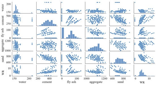
Figure 1.
Correlation between the factors (Unit: kg/m3).
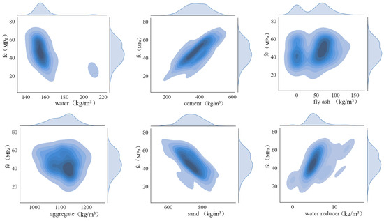
Figure 2.
Influence of each factor on compressive strength.
The correlation coefficients between input parameters and CS were calculated, as shown in Figure 3. The correlation between water and water reducer is higher comparing with the others and shows an obvious negative trend; then, the correlation between cement and sand is the second highest. The reason is that sand and coarse aggregate show a negative correlation. Therefore, the more sand, the less coarse aggregate, and the less cement is used in general; the fly ash was added to concrete in a way that partially replaces cement, so the correlation between them is relatively higher.
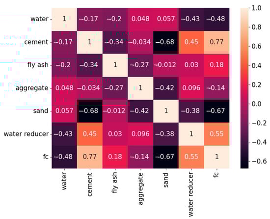
Figure 3.
Correlation coefficient between the factors.
As for the correlation between the compressive strength and each input parameter, the water, cement and sand are much higher than the others; among them, the influence of water and sand on compressive strength is negative, while the influence of cement on compressive strength is positive. However, the hardening effect of fly ash occurs late [43], so the effect of fly ash on the CS of concrete is small.
3. Machine Learning Algorithms
Machine learning (ML) algorithms have advantages in big data processing, regression and image recognition, and many researchers have applied ML algorithms to scientific research [44,45,46]. In this study, a variety of regression algorithms based on ML technology, including two NN-based algorithms, two assembled algorithms, SVR and GP were used to predict the 7-day CS of concrete containing FA. The accuracy of each model is discussed comprehensively based on various statistical indicators. Figure 4 shows the flowchart of this study.
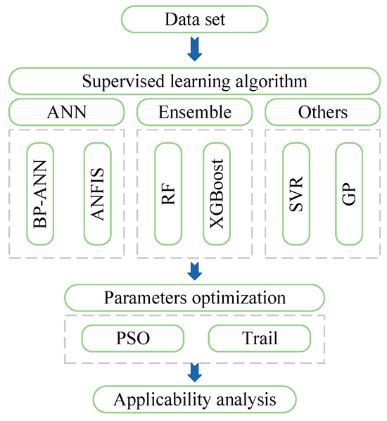
Figure 4.
Flowchart of the research.
3.1. PSO Algorithm
PSO is a metaheuristic algorithm. In this algorithm, the potential solution to the problem is to be regarded as a bird (particle) in the flock; each bird has its own speed and position. It is characterized by the ability to update the speed and position of the particle based on the particle’s memory of its own historical optimal solution (extreme value) and the experience shared by the entire population (global extreme value); the characteristic is formulaic, as shown in Equations (2) and (3).
where the subscript D indicates that there is a D-dimensional search space that is the number of indicators to be searched; represents the velocity of the i particle in the D; represents the position of the particle; and represent the individual extremum and global extremum, respectively; is the inertia weight, and the value usually takes 1; and are the acceleration constant, which usually take ; and and are the random numbers generated from the interval [0, 1].
The hyperparameters of an ML algorithm have a significant impact on its prediction accuracy, while manual adjustment is cumbersome and time-consuming, thus significantly reducing the efficiency of an ML algorithm. Therefore, in this study, a PSO optimization algorithm is used to automatically find the best value of hyperparameters that have an important influence in each ML algorithm.
However, ANFIS requires huge random access memory on the part of the computer in the operation process, so it is not suitable for PSO to optimize its hyperparameters across a wide range. Moreover, the most influential hyperparameters of ANFIS are the type and number of membership functions and membership grade, so the hyperparameter optimization of ANFIS used trial and error. In addition, the hyperparameters of the others standalone ML algorithms adopted their default values or the literature recommendations. The specific hyperparameters of each hybrid and standalone ML model are shown in Table 2 and Table 3.
Table 2.
Hyperparameters setting of the standalone models.
Table 3.
Searched hyperparameters of each predicting model.
3.2. BP-ANN
BP-ANN is a computational system built by imitating the operation mode of neurons [47]. It is usually composed of an input layer, hidden layer and output layer, and its operation mode is mainly composed of forward propagation and backpropagation.
In forward propagation, the data of each input parameter are first input into the neurons of the “input layer”, and then the input data are transmitted to the next neuron through a certain logical relationship, as shown in Equation (4), and finally to the neurons of the “output layer”.
This logical relationship includes the weight wij of the I neuron of the k layer to the j neuron of the k + 1 layer (k is the number of the layers, including the input layer and the hidden layers), and the bias bi of the k layer neuron. The received data of the k + 1 layer will be processed by the activation function; then, the data will be transformed to the k + 2 layer.
In backpropagation, the predicted value y, obtained through the aforementioned logical relationship, is compared with the experimental value y, and the loss function is obtained, so the gradient function of the loss function can be obtained. Finally, the weight and bias are constantly transformed through the gradient descent algorithm, and the optimal weight vector and the bias of each layer are finally obtained.
3.3. ANFIS
This method combines a neural network with fuzzy logic to classify the data. This fuzzy classification ability enables the computer to understand the input data, and then it has a higher ability to resist data error and excellent prediction performance [36].
ANFIS models are usually divided into five layers:
- (1)
- The first layer is the fuzzy layer, which undertakes fuzzy processing of input data by membership function. The selection of the type and number of membership function is usually subjective. When there are more membership functions of each input parameter, there will also be more membership degrees, so more if–then rules will be generated, which may improve the prediction accuracy to a certain level but also significantly increase the requirement of computer performance.
- (2)
- The second layer is to calculate the firing strength of each if–then rule.
- (3)
- The third layer normalizes the firing strength and obtains the trigger intensity of the if–then rule relative to the others.
- (4)
- The fourth layer calculates the output value of each if–then rule by multiplying the original input data and the relative trigger intensity obtained in the third layer.
- (5)
- The fifth layer is the output layer, which weights and sums the output values obtained in the fourth layer and defuzzies them.
Since the final output result is weighted and summed, it also means that the predicted target can only be a single variable, and it is impossible to achieve a multi-variable output.
3.4. SVR
The support vector machine (SVM) is proposed by Vapnik et al. [48]; the algorithm used for regression is support vector regression (SVR), whose main idea is to construct an interval band that can accommodate as many data points as possible, while minimizing the loss of data points that are not in the interval band.
Data points in the interval band are not counted for their loss, and SVR maps the data to the feature space by kernel function, which makes the nonlinear regression problem become a linear regression problem approximately. Therefore, the advantages of SVR include high generalization, being iterative fast, global optimization and avoidance of local minimization [19,49]. In addition, SVR has an excellent fitting performance in nonlinear regression problems with multiple variables and small data.
3.5. XGBoost
XGBoost is an algorithm based on a boosting framework. Boosting is an addition model that includes multiple estimators, each of which gives a set of predicted values, and the latter estimator will learn the deviation between the previous estimator’s predicted value and experimental value, and then continuously reduces the deviation.
3.6. RF
Random forest is an assembled machine learning algorithm based on a bagging framework, which combines multiple decision trees. Bagging is to randomly extract n samples from the database and form a new training set. According to the above method, M new training sets are generated according to the assembled M decision trees; each decision tree gives a set of prediction values base on its training set, and then M prediction results are obtained. Finally, the average of these M prediction results is used as the final prediction result.
3.7. GP
Genetic programming is an evolutionary algorithm designed to fit data sets by giving a mathematical expression that approximates the relationship between features and target. Unlike others regression ML algorithms, GP can construct a mathematical expression by searching and combining basic mathematical operators, features and constants. Therefore, GP is also one of the few interpretable ML algorithms, that is, one giving exact mathematical expressions.
4. Results and Discussions
4.1. Prediction Performance of Standalone Models
R2, MSE, MAE and explanatory variance were used to evaluate the prediction accuracy of the constructed algorithms. The statistic indexes were calculated using the r2_score, mean_absolute_error, mean_squared_error and sm.taylor functions in the sklearn.metrics library.
The prediction results of each standalone model are shown in Figure 5, Figure 6, Figure 7, Figure 8, Figure 9 and Figure 10. MSE represents the degree of error between the predicted and experimental value. At the same time, the weight of large error will be highlighted after the squared, so it is more sensitive to the error than other statistical indexes. Although the prediction error of the testing set was slightly higher than that of the training set, the standalone model still had acceptable MSE values except GP and ANFIS.
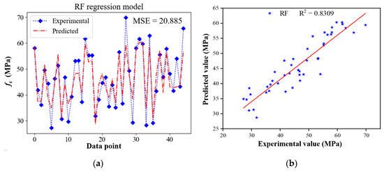
Figure 5.
Prediction results of RF model for test set: (a) Error and (b) correlation between predicted value and experimental value.
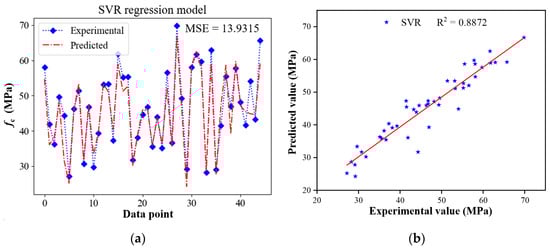
Figure 6.
Prediction results of SVR model for test set: (a) Error and (b) correlation between predicted value and experimental value.
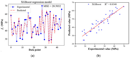
Figure 7.
Prediction results of XGBoost model for test set: (a) Error and (b) correlation between predicted value and experimental value.
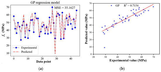
Figure 8.
Prediction results of GP model for test set: (a) Error and (b) correlation between predicted value and experimental value.
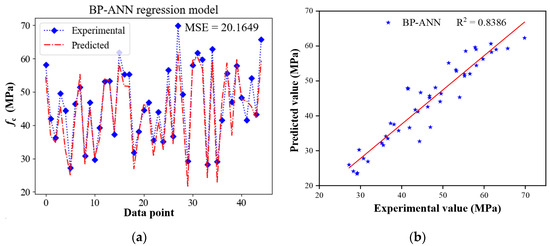
Figure 9.
Prediction results of BP-ANN model for test set: (a) Error and (b) correlation between predicted value and experimental value.
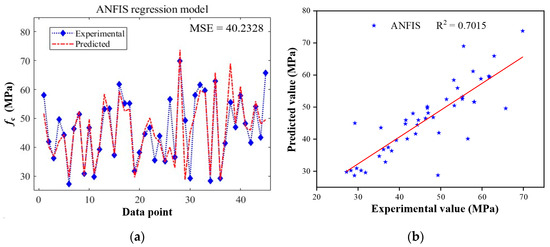
Figure 10.
Prediction results of ANFIS model for test set: (a) Error and (b) correlation between predicted value and experimental value.
The R2 indicates the fitness of prediction of the model. As can be seen from the figure, the R2 of the predicted and experimental values is generally around 0.8, indicating the selected ML algorithms have a good predicting performance. However, the R2 of AFNIS and GP are only 0.7015 and 0.7154, respectively. The prediction ability of the GP model is dependent on variability, just like genetic variation [26]. Therefore, the variation direction of branches is highly controlled by the hyperparameter settings. In contrast, SVR has the highest R2 by virtue of its excellent generalization. As for RF and XGBoost models, their fitting goodness showed a certain fluctuation, and this is because of their random splitting of tree branches and the formation of data subsets of each sub-tree integrated in them, and all of this results in a decisive dependency on the hyperparameter setting. As a contrast, the SVR model will map the lower dimension problem to the higher one and simplify the calculation through kernel function, performing little randomness. Therefore, the SVR model is outperformed. The ANFIS showed a worse R2; this may because the database has six features, resulting in the requirement of many more membership degrees (MDs), and the MDs only default at two for each feature, resulting in the poor performance of the ANFIS model.
4.2. Prediction Performance of Hybrid Models
The prediction value and performance of the hybrid models are shown in Figure 11, Figure 12, Figure 13, Figure 14, Figure 15 and Figure 16. After PSO optimization, the prediction accuracy of each model has been significantly improved. MSE and R2 of PSO-RF are 11.9172 and 0.9035, respectively, which are 42.9% lower and 8.7% higher than that of RF, respectively; while for PSO-SVR, the MSE and R2 are reduced 14.8% and increased 1.9% compared with its standalone model; for XGBoost, the results are 44.1% and 8.9%; for GP, they are 56.2% and 22.4%; and for BP-ANN, they are 16% and 2.9%.
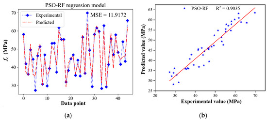
Figure 11.
Prediction results of PSO-RF model for test set: (a) Error and (b) correlation between predicted value and experimental value.
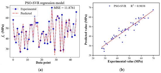
Figure 12.
Prediction results of PSO-SVR model for test set: (a) Error and (b) correlation between predicted value and experimental value.
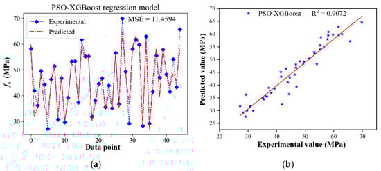
Figure 13.
Prediction results of PSO-XGBoost model for test set: (a) Error and (b) correlation between predicted value and experimental value.
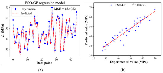
Figure 14.
Prediction results of PSO-GP model for test set: (a) Error and (b) correlation between predicted value and experimental value.
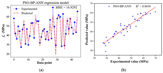
Figure 15.
Prediction results of PSO-BP-ANN model for test set: (a) Error and (b) correlation between predicted value and experimental value.
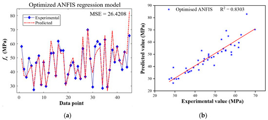
Figure 16.
Prediction results of optimized ANFIS model for test set: (a) Error and (b) correlation between predicted value and experimental value.
Among them, the GP model improved the most after PSO optimization, which indicates that hyperparameters have a greater impact on the GP model to a certain extent. At the same time, PSO has the smallest improvement on the SVR model, which is because the SVR model has a high generalization, so the impact of data quality and model setting on its prediction accuracy is relatively low. The PSO-XGBoost model has the lowest error and the highest fitness, with an MSE of 11.4594 and R2 of 0.9072. In addition, the assembled and SVR algorithms have better prediction performance than the NN-based algorithms.
The optimization of the ANFIS model used trial and error due to its high requirements on computer performance. Under the condition that there are no more than three membership grades for each input parameter, the membership grade combination of 2-3-2-3-1 with Gaussian function was finally determined. After the optimization, the MSE was reduced by 34.3%, and the R2 was increased by 18.4%. As aforementioned, the predicting performance of RF and XGBoost is highly dependent on the hyperparameter setting. Therefore, the predicting accuracy is significantly increased.
4.3. Analysis of Error Distribution
The absolute error distribution of each model is shown in Figure 17, Figure 18, Figure 19, Figure 20, Figure 21 and Figure 22. After PSO optimization, the maximum absolute error of each model is reduced to some extent. However, the distribution of red noise in the RF, XGBoost, ANFIS and BP-ANN models is relatively scattered, indicating that there are many large error points in the range of predicted data. In contrast, the error distribution of SVR and PSO-GP is more uniform in the predicted data range, so there are fewer large error points.
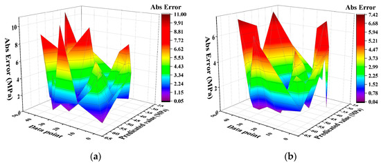
Figure 17.
Error distribution of RF algorithm (a) RF; (b) PSO-RF.
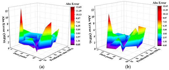
Figure 18.
Error distribution of SVR algorithm (a) SVR; (b) PSO-SVR.
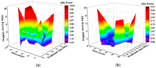
Figure 19.
Error distribution of XGBoost algorithm (a) XGBoost; (b) PSO-XGBoost.
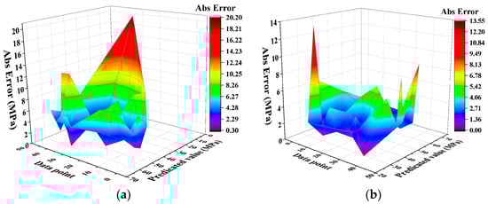
Figure 20.
Error distribution of GP algorithm (a) GP; (b) PSO-GP.
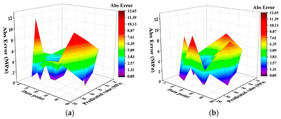
Figure 21.
Error distribution of BP-ANN algorithm (a) BP-ANN; (b) PSO-BP-ANN.
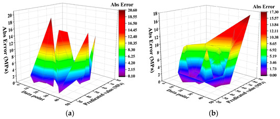
Figure 22.
Error distribution of ANFIS algorithm (a) ANFIS; (b) optimized ANFIS.
Although RF and XGBoost have a higher R2 and lower MSE after PSO optimization, they have more large error points, which may lead to larger prediction errors in practical applications. Therefore, SVR and PSO-GP are more suitable for regression prediction of this data set.
It is worth noting that the prediction accuracy of the GP model is relatively lower, but the absolute error distribution is more uniform, indicating that there are fewer relatively large error points in its prediction results, which indicates that the GP model has good prediction potential for this data set.
4.4. Accuracy Analysis
The statistical indicators of the predicted and experimental values of each model are summarized in Table 4. The R2 of the optimized ANFIS is only 4.5% and 0.7% lower than XGBoost and RF, respectively, but the MSE is 29.6% and 27.7% higher. In addition, the change rates of R2 and MSE of each model are significantly different after PSO optimization. The reason is that different statistic indicators have different sensitivity to the errors. Therefore, it is difficult to fully reflect the prediction accuracy of the model through a single statistical indicator.
Table 4.
Statistic indexes of each model.
In view of this, a Taylor diagram was used to combine several statistical indicators to comprehensively evaluate the prediction accuracy of each model. According to Equation (5), the R, RMSE and standard deviation (STD) of the predicted value and experimental value are combined in the two-dimensional plane graph. The comprehensive evaluation of each model is shown in Figure 23.
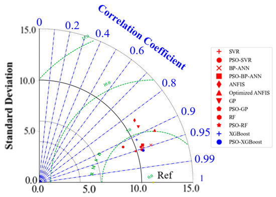
Figure 23.
Taylor diagram for each model.
The blue dot–dash line represents the R, the green dash line represents the RMSE and the black dotted line represents the standard deviation. The distance between each point to Ref represents the comprehensive performance of each ML model; a shorter distance means a higher comprehensive performance. As can be seen from the figure, PSO-XBGoost has the best comprehensive performance.
5. Conclusions
To build a compressive strength prediction model for fly ash concrete, this study selected two assembled algorithms, two NN-based algorithms and machine learning algorithms. The PSO algorithm was also used to optimize the structure or hyperparameters of the above ML algorithms. Finally, the predicting performance of each model was evaluated using statistical indicators. The main conclusions of this study are as follows:
- (1)
- As a standalone model, the SVR algorithm has the highest R2 of 0.8837 and lowest MSE of 13.9315 with good generalization. In addition, the assembled algorithm outperforms the NN-based algorithm.
- (2)
- The PSO algorithm can effectively improve the prediction accuracy of all the ML models. Among them, the improvement in prediction accuracy of GP is the highest; its MSE decreased by 56.2% and R2 increased by 22.4% after cooperating with PSO. In addition, the R2 of the PSO-RF, PSO-XGBoost and PSO-SVR models are all greater than 0.9.
- (3)
- The absolute error distribution of the PSO-GP and SVR algorithms is relatively uniform, which means that there are fewer large error points in their prediction results, so it is not easy to have a large prediction error under a certain set of features. According to the statistical indicators of each standalone and hybrid algorithm, PSO-XGBoost has the best comprehensive performance.
- (4)
- Given the specificity of each predicting scenario, the same predicting models which have an appropriate accuracy in the fc prediction may not have performed excellently in the other scenarios such as anti-chloride diffusion, carbonization and so forth. Therefore, the applicability of each model should be carefully discussed in the others’ predicting scenarios.
- (5)
- Although six different machine learning algorithms were used to predict the fc of the concrete containing coal fly ash, the kinds of machine learning algorithms are still limited. Future research could discuss the applicability of other machine learning algorithms, even constructing a synthesizing operational interface to improve usability in the field.
Author Contributions
Conceptualization, Y.Z. and X.Y.; Data curation, Y.Z.; Formal analysis, H.Z.; Methodology, Y.Y. and G.L.; Resources, H.Z.; Software, Y.Y. and G.L.; Writing—original draft, G.L. All authors have read and agreed to the published version of the manuscript.
Funding
The research was funded by the Fund of Small and Medium Enterprise Innovation Project of Gansu Provincial Department of Science and Technology (22CX3GA073).
Data Availability Statement
The data presented in this study are available on request from the corresponding author. The data are not publicly available due to privacy.
Conflicts of Interest
Author Yanhua Yang, Haihong Zhang and Yan Zhang were employed by the company Gansu Provincial Transportation Research Institute Group Co., Ltd. The remaining authors declare that the research was conducted in the absence of any commercial or financial relationships that could be construed as a potential conflict of interest.
References
- Sahoo, S.; Mahapatra, T.R. ANN Modeling to study strength loss of Fly Ash Concrete against Long term Sulphate Attack. Mater. Today Proc. 2018, 5, 24595–24604. [Google Scholar] [CrossRef]
- Mohamed, O.; Kewalramani, M.; Ati, M.; Hawat, W.A. Application of ANN for prediction of chloride penetration resistance and concrete compressive strength. Materialia 2021, 17, 101123. [Google Scholar] [CrossRef]
- Mohamed, O.A.; Najm, O.F. Compressive strength and stability of sustainable self-consolidating concrete containing fly ash, silica fume, and GGBS. Front. Struct. Civ. Eng. 2017, 11, 406–411. [Google Scholar] [CrossRef]
- Huang, H.; Yuan, Y.J.; Zhang, W.; Zhu, L. Property Assessment of High-Performance Concrete Containing Three Types of Fibers. Int. J. Concr. Struct. Mater. 2021, 15, 39. [Google Scholar] [CrossRef]
- Zheng, Z.; Tian, C.; Wei, X.; Zeng, C. Numerical investigation and ANN-based prediction on compressive strength and size effect using the concrete mesoscale concretization model. Case Stud. Constr. Mater. 2022, 16, e01056. [Google Scholar] [CrossRef]
- Ullah, H.S.; Khushnood, R.A.; Farooq, F.; Ahmad, J.; Vatin, N.I.; Ewais, D.Y. Prediction of Compressive Strength of Sustainable Foam Concrete Using Individual and Ensemble Machine Learning Approaches. Materials 2022, 15, 3166. [Google Scholar] [CrossRef] [PubMed]
- Khan, M.A.; Farooq, F.; Javed, M.F.; Zafar, A.; Ostrowski, K.A.; Aslam, F.; Malazdrewicz, S.; Maślak, M. Simulation of Depth of Wear of Eco-Friendly Concrete Using Machine Learning Based Computational Approaches. Materials 2022, 15, 58. [Google Scholar] [CrossRef]
- Petković, D.; Ćojbašić, Ž.; Nikolić, V.; Shamshirband, S.; Mat Kiah, M.L.; Anuar, N.B.; Abdul Wahab, A.W. Adaptive neuro-fuzzy maximal power extraction of wind turbine with continuously variable transmission. Energy 2014, 64, 868–874. [Google Scholar] [CrossRef]
- Shamshirband, S.; Petković, D.; Amini, A.; Anuar, N.B.; Nikolić, V.; Ćojbašić, Ž.; Mat Kiah, M.L.; Gani, A. Support vector regression methodology for wind turbine reaction torque prediction with power-split hydrostatic continuous variable transmission. Energy 2014, 67, 623–630. [Google Scholar] [CrossRef]
- Petković, B.; Agdas, A.S.; Zandi, Y.; Nikolić, I.; Denić, N.; Radenkovic, S.D.; Almojil, S.F.; Roco-Videla, A.; Kojić, N.; Zlatković, D.; et al. Neuro fuzzy evaluation of circular economy based on waste generation, recycling, renewable energy, biomass and soil pollution. Rhizosphere 2021, 19, 100418. [Google Scholar] [CrossRef]
- Nguyen, T.-D.; Cherif, R.; Mahieux, P.-Y.; Lux, J.; Aït-Mokhtar, A.; Bastidas-Arteaga, E. Artificial intelligence algorithms for prediction and sensitivity analysis of mechanical properties of recycled aggregate concrete: A review. J. Build. Eng. 2023, 66, 105929. [Google Scholar] [CrossRef]
- Taffese, W.Z.; Sistonen, E.; Puttonen, J. CaPrM: Carbonation prediction model for reinforced concrete using machine learning methods. Constr. Build. Mater. 2015, 100, 70–82. [Google Scholar] [CrossRef]
- Adeli, H.; Cheng, N.T. Integrated Genetic Algorithm for Optimization of Space Structures. J. Aerosp. Eng. 1993, 6, 315–328. [Google Scholar] [CrossRef]
- Xu, J.; Wang, Y.; Ren, R.; Wu, Z.; Ozbakkaloglu, T. Performance evaluation of recycled aggregate concrete-filled steel tubes under different loading conditions: Database analysis and modelling. J. Build. Eng. 2020, 30, 101308. [Google Scholar] [CrossRef]
- Dantas, A.T.A.; Batista Leite, M.; de Jesus Nagahama, K. Prediction of compressive strength of concrete containing construction and demolition waste using artificial neural networks. Constr. Build. Mater. 2013, 38, 717–722. [Google Scholar] [CrossRef]
- Huang, W.; Zhou, L.; Ge, P.; Yang, T. A Comparative Study on Compressive Strength Model of Recycled Brick Aggregate Concrete Based on PSO-BP and GA-BP Neural Networks. Mater. Rep. 2021, 35, 15026–15030. (In Chinese) [Google Scholar]
- Ahmadi, M.; Kioumarsi, M. Predicting the elastic modulus of normal and high strength concretes using hybrid ANN-PSO. Mater. Today Proc. 2023, in press. [Google Scholar] [CrossRef]
- Kim, S.; Choi, H.-B.; Shin, Y.; Kim, G.-H.; Seo, D.-S. Optimizing the Mixing Proportion with Neural Networks Based on Genetic Algorithms for Recycled Aggregate Concrete. Adv. Mater. Sci. Eng. 2013, 2013, 527089. [Google Scholar] [CrossRef]
- Zheng, W.; Zaman, A.; Farooq, F.; Althoey, F.; Alaskar, A.; Akbar, A. Sustainable predictive model of concrete utilizing waste ingredient: Individual alogrithms with optimized ensemble approaches. Mater. Today Commun. 2023, 35, 105901. [Google Scholar] [CrossRef]
- Ababneh, A.; Alhassan, M.; Abu-Haifa, M. Predicting the contribution of recycled aggregate concrete to the shear capacity of beams without transverse reinforcement using artificial neural networks. Case Stud. Constr. Mater. 2020, 13, e00414. [Google Scholar] [CrossRef]
- Jin, L.; Dong, T.; Fan, T.; Duan, J.; Yu, H.; Jiao, P.; Zhang, W. Prediction of the chloride diffusivity of recycled aggregate concrete using artificial neural network. Mater. Today Commun. 2022, 32, 104137. [Google Scholar] [CrossRef]
- Hiew, S.Y.; Teoh, K.B.; Raman, S.N.; Kong, D.; Hafezolghorani, M. Prediction of ultimate conditions and stress–strain behaviour of steel-confined ultra-high-performance concrete using sequential deep feed-forward neural network modelling strategy. Eng. Struct. 2023, 277, 115447. [Google Scholar] [CrossRef]
- Minaz Hossain, M.; Nasir Uddin, M.; Abu Sayed Hossain, M. Prediction of compressive strength ultra-high steel fiber reinforced concrete (UHSFRC) using artificial neural networks (ANNs). Mater. Today Proc. 2023, in press. [Google Scholar] [CrossRef]
- Allouzi, R.; Almasaeid, H.; Alkloub, A.; Ayadi, O.; Allouzi, R.; Alajarmeh, R. Lightweight foamed concrete for houses in Jordan. Case Stud. Constr. Mater. 2023, 18, e01924. [Google Scholar] [CrossRef]
- Kursuncu, B.; Gencel, O.; Bayraktar, O.Y.; Shi, J.; Nematzadeh, M.; Kaplan, G. Optimization of foam concrete characteristics using response surface methodology and artificial neural networks. Constr. Build. Mater. 2022, 337, 127575. [Google Scholar] [CrossRef]
- Salami, B.A.; Iqbal, M.; Abdulraheem, A.; Jalal, F.E.; Alimi, W.; Jamal, A.; Tafsirojjaman, T.; Liu, Y.; Bardhan, A. Estimating compressive strength of lightweight foamed concrete using neural, genetic and ensemble machine learning approaches. Cem. Concr. Compos. 2022, 133, 104721. [Google Scholar] [CrossRef]
- Asteris, P.G.; Lourenço, P.B.; Roussis, P.C.; Elpida Adami, C.; Armaghani, D.J.; Cavaleri, L.; Chalioris, C.E.; Hajihassani, M.; Lemonis, M.E.; Mohammed, A.S.; et al. Revealing the nature of metakaolin-based concrete materials using artificial intelligence techniques. Constr. Build. Mater. 2022, 322, 126500. [Google Scholar] [CrossRef]
- Bhuva, P.; Bhogayata, A.; Kumar, D. A comparative study of different artificial neural networks for the strength prediction of self-compacting concrete. Mater. Today Proc. 2023. [Google Scholar] [CrossRef]
- Gao, X.; Yang, J.; Zhu, H.; Xu, J. Estimation of rubberized concrete frost resistance using machine learning techniques. Constr. Build. Mater. 2023, 371, 130778. [Google Scholar] [CrossRef]
- Naseri Nasab, M.; Jahangir, H.; Hasani, H.; Majidi, M.-H.; Khorashadizadeh, S. Estimating the punching shear capacities of concrete slabs reinforced by steel and FRP rebars with ANN-Based GUI toolbox. Structures 2023, 50, 1204–1221. [Google Scholar] [CrossRef]
- Bardhan, A.; Biswas, R.; Kardani, N.; Iqbal, M.; Samui, P.; Singh, M.P.; Asteris, P.G. A novel integrated approach of augmented grey wolf optimizer and ANN for estimating axial load carrying-capacity of concrete-filled steel tube columns. Constr. Build. Mater. 2022, 337, 127454. [Google Scholar] [CrossRef]
- Zhao, B.; Li, P.; Du, Y.; Li, Y.; Rong, X.; Zhang, X.; Xin, H. Artificial neural network assisted bearing capacity and confining pressure prediction for rectangular concrete-filled steel tube (CFT). Alex. Eng. J. 2023, 74, 517–533. [Google Scholar] [CrossRef]
- Concha, N.C. Neural network model for bond strength of FRP bars in concrete. Structures 2022, 41, 306–317. [Google Scholar] [CrossRef]
- Huang, L.; Chen, J.; Tan, X. BP-ANN based bond strength prediction for FRP reinforced concrete at high temperature. Eng. Struct. 2022, 257, 114026. [Google Scholar] [CrossRef]
- Zhang, F.; Wang, C.; Liu, J.; Zou, X.; Sneed, L.H.; Bao, Y.; Wang, L. Prediction of FRP-concrete interfacial bond strength based on machine learning. Eng. Struct. 2023, 274, 115156. [Google Scholar] [CrossRef]
- You, X.; Yan, G.; Al-Masoudy, M.M.; Kadimallah, M.A.; Alkhalifah, T.; Alturise, F.; Ali, H.E. Application of novel hybrid machine learning approach for estimation of ultimate bond strength between ultra-high performance concrete and reinforced bar. Adv. Eng. Softw. 2023, 180, 103442. [Google Scholar] [CrossRef]
- Sun, L.; Wang, C.; Zhang, C.W.; Yang, Z.Y.; Li, C.; Qiao, P.Z. Experimental investigation on the bond performance of sea sand coral concrete with FRP bar reinforcement for marine environments. Adv. Struct. Eng. 2023, 26, 533–546. [Google Scholar] [CrossRef]
- Gehlot, T.; Dave, M.; Solanki, D. Neural network model to predict compressive strength of steel fiber reinforced concrete elements incorporating supplementary cementitious materials. Mater. Today Proc. 2022, 62, 6498–6506. [Google Scholar] [CrossRef]
- Fakharian, P.; Rezazadeh Eidgahee, D.; Akbari, M.; Jahangir, H.; Ali Taeb, A. Compressive strength prediction of hollow concrete masonry blocks using artificial intelligence algorithms. Structures 2023, 47, 1790–1802. [Google Scholar] [CrossRef]
- Owusu-Danquah, J.S.; Bseiso, A.; Allena, S.; Duffy, S.F. Artificial neural network algorithms to predict the bond strength of reinforced concrete: Coupled effect of corrosion, concrete cover, and compressive strength. Constr. Build. Mater. 2022, 350, 128896. [Google Scholar] [CrossRef]
- Rehman, F.; Khokhar, S.A.; Khushnood, R.A. ANN based predictive mimicker for mechanical and rheological properties of eco-friendly geopolymer concrete. Case Stud. Constr. Mater. 2022, 17, e01536. [Google Scholar] [CrossRef]
- Sadowski, Ł.; Hoła, J. ANN modeling of pull-off adhesion of concrete layers. Adv. Eng. Softw. 2015, 89, 17–27. [Google Scholar] [CrossRef]
- Imran Waris, M.; Plevris, V.; Mir, J.; Chairman, N.; Ahmad, A. An alternative approach for measuring the mechanical properties of hybrid concrete through image processing and machine learning. Constr. Build. Mater. 2022, 328, 126899. [Google Scholar] [CrossRef]
- Nikolić, V.; Mitić, V.V.; Kocić, L.; Petković, D. Wind speed parameters sensitivity analysis based on fractals and neuro-fuzzy selection technique. Knowl. Inf. Syst. 2017, 52, 255–265. [Google Scholar] [CrossRef]
- Wang, Q.; Xia, C.; Alagumalai, K.; Thanh Nhi Le, T.; Yuan, Y.; Khademi, T.; Berkani, M.; Lu, H. Biogas generation from biomass as a cleaner alternative towards a circular bioeconomy: Artificial intelligence, challenges, and future insights. Fuel 2023, 333, 126456. [Google Scholar] [CrossRef]
- Cao, B.T.; Obel, M.; Freitag, S.; Mark, P.; Meschke, G. Artificial neural network surrogate modelling for real-time predictions and control of building damage during mechanised tunnelling. Adv. Eng. Softw. 2020, 149, 102869. [Google Scholar] [CrossRef]
- Felix, E.F.; Carrazedo, R.; Possan, E. Carbonation model for fly ash concrete based on artificial neural network: Development and parametric analysis. Constr. Build. Mater. 2021, 266, 121050. [Google Scholar] [CrossRef]
- Payton, E.; Khubchandani, J.; Thompson, A.; Price, J.H. Parents’ Expectations of High Schools in Firearm Violence Prevention. J. Community Health 2017, 42, 1118–1126. [Google Scholar] [CrossRef]
- Çevik, A.; Kurtoğlu, A.E.; Bilgehan, M.; Gülşan, M.E.; Albegmprli, H.M. Support vector machines in structural engineering: A review. J. Civ. Eng. Manag. 2015, 21, 261–281. [Google Scholar] [CrossRef]
Disclaimer/Publisher’s Note: The statements, opinions and data contained in all publications are solely those of the individual author(s) and contributor(s) and not of MDPI and/or the editor(s). MDPI and/or the editor(s) disclaim responsibility for any injury to people or property resulting from any ideas, methods, instructions or products referred to in the content. |
© 2024 by the authors. Licensee MDPI, Basel, Switzerland. This article is an open access article distributed under the terms and conditions of the Creative Commons Attribution (CC BY) license (https://creativecommons.org/licenses/by/4.0/).