Analytical Solution for the Steady Seepage Field of an Anchor Circular Pit in Layered Soil

Abstract

An analytical study was carried out on an anchored circular pit with a submerged free surface in layered soil. The seepage field around the anchor circular pit was divided into three zones. Separate variable method was used to obtain the graded solution forms of head distribution in the column coordinate system for each of the three regions. Combined with the continuity condition between the regions the Bessel function orthogonality was used to obtain the explicit analytical solution of the seepage field in each region, and the infiltration line was determined. Comparison with the calculation results of Plaxis 2D 8.5 software verified the correctness of the analytical solution. Based on the analytical solution, the influence of the radius of the pit and the distance of the retaining wall from the top surface of the impermeable layer on the total head distribution on both sides of the retaining wall was analyzed. And the variation in the infiltration line was determined with the above parameters. The results show that as the pit radius, r, decreased, the total head on both sides of the retaining wall gradually increased, and the height of the submerged surface drop also increased. As the distance, a, between the retaining wall and the impermeable boundary at the bottom increased, the hydraulic head on the outer side of the retaining wall decreased and the head on the inner side increased. The height of the submerged surface drop increased with decreasing depth of insertion of the retaining wall. The depth of insertion of the retaining wall had a greater influence on the degree of diving surface drop than the pit radius.

1. Introduction

Round or circular anchor pits are often encountered in bridge piers, housing buildings, port overturning engine houses, and other projects, and with the size and depth of pits increasing, anchor pit projects present many new and urgent problems in construction. Groundwater seepage has a significant impact on the stability and deformation of foundation pit projects, and the data suggest that seepage action is the main cause of many foundation pit project failures [1]. Due to thick aquifers or for technical and economic reasons, suspended retaining walls are often used for the design of anchor pits, but the impermeability of the retaining walls, as well as the flow-around characteristics at the base of the walls, makes the seepage pattern of anchor circular pits present a special complexity. In order to reduce the engineering risk and assess the possible hazards, foundation stability analysis, calculation of foundation seepage volumes and infiltration pressures in various parts of the seepage field, and determination of infiltration line locations are required. Determining the location of the infiltration line is one of the core tasks.

At present, research in the groundwater seepage field mainly includes numerical calculation and analytical methods. With the gradual maturation of numerical analysis, many scholars use numerical methods such as finite element and finite difference to analyze the seepage of foundation pit projects under steady and transient seepage regimes, which can obtain more accurate head solutions [2]. Compared with numerical calculation and the approximate method, the analytical method can incorporate factors such as initial groundwater conditions and water level changes into the solution process and express each factor through a functional expression, which facilitates the further study of groundwater movement laws. Some scholars have approximated the seepage from a pit into a two-dimensional (2D) problem for a rectangular pit of relatively large length and width, where the water level outside the pit is a constant level. For example, Fox and McNamee (1942) [3] used Schwarz–Christofel’s transformation method to derive an analytical solution for 2D seepage flow at a constant head difference between the inside and outside of the pit, and Bereslavskii (2011) [4] gave an analytical solution for steady-state seepage flow around a single sheet pile wall at a constant water level based on the angle-preserving transformation method. Banerjee (1992) [5] used the continuous angle-preserving transformation method to obtain a series of implicit expressions for the seepage elements around a foundation pit. The existing angle-preserving transformation methods all consider the seepage field of the pit as a whole, which requires the establishment of complex correspondence between irregular and regular boundaries, and can only obtain implicit analytical solutions for the seepage in the pit. Huang (2014) [2] used the Fourier transform to give a semi-analytical solution for the two-dimensional steady-state seepage flow in the pit by partitioning the seepage field around the pit, but the solution for the hydraulic gradient in the calculation process uses a discrete method, and only an approximate solution can be obtained, and there are still errors and deficiencies in the simulation of the seepage flow in the pit.

The seepage pattern of an anchor circular pit is quite different from that of a rectangular pit and is difficult to resolve by means of angle-preserving transformations [6]. In addition, a certain depth of water level drop is generated around the anchorage pit, forming a free boundary of the diving surface that is both a flow line and an isobaric line, and the non-linearity of the free boundary conditions (due to the squared value of the hydraulic gradient) hinders the conventional solution of the linear Laplace equation. Therefore, there are fewer research results on the analysis of the seepage field for anchor circular pits. Wang (2015) [7] used Dupuit’s equation and barrier theory to propose a modified large well method to derive the expression for the influx of water in suspended curtain circular pits. Lin (2013) [8] studied a submerged aquifer along the dive level maximum depth of drop into the upper and lower parts, using the integral transformation method; the derived steady flow formula can be applied to different tube lengths and submerged states of constant flow in a submerged layer of a non-complete well and can also be applied to the calculation of the foundation pit project surge. Most of the above studies are based on certain approximate assumptions, and there are few studies on the analysis of seepage flow in circular pits in a more rigorous sense considering the depth of the water level drop.

In this paper, a mathematical model of steady-state seepage in an anchor circular pit in layered soil is constructed based on reasonable assumptions, and the analytical solution of the model is obtained through a series of mathematical methods. The analytical solution can represent the head distribution of the seepage field and can also solve the excavation surface seepage volume, hydraulic gradient, and other parameters. In addition, the analytical solution also takes into account the water level drop depth and is able to solve the infiltration line. Several calculation examples are used to compare the results of the analytical solution with the numerical simulation results, and the two results match well, which fully proves the correctness of the analytical solution. On this basis, the influence of parameters such as the radius of the pit, the distance from the pit retaining wall to the impermeable layer, and the water level inside the retaining wall on the head and depth of the water level drop are further analyzed.

2. Problem Definition

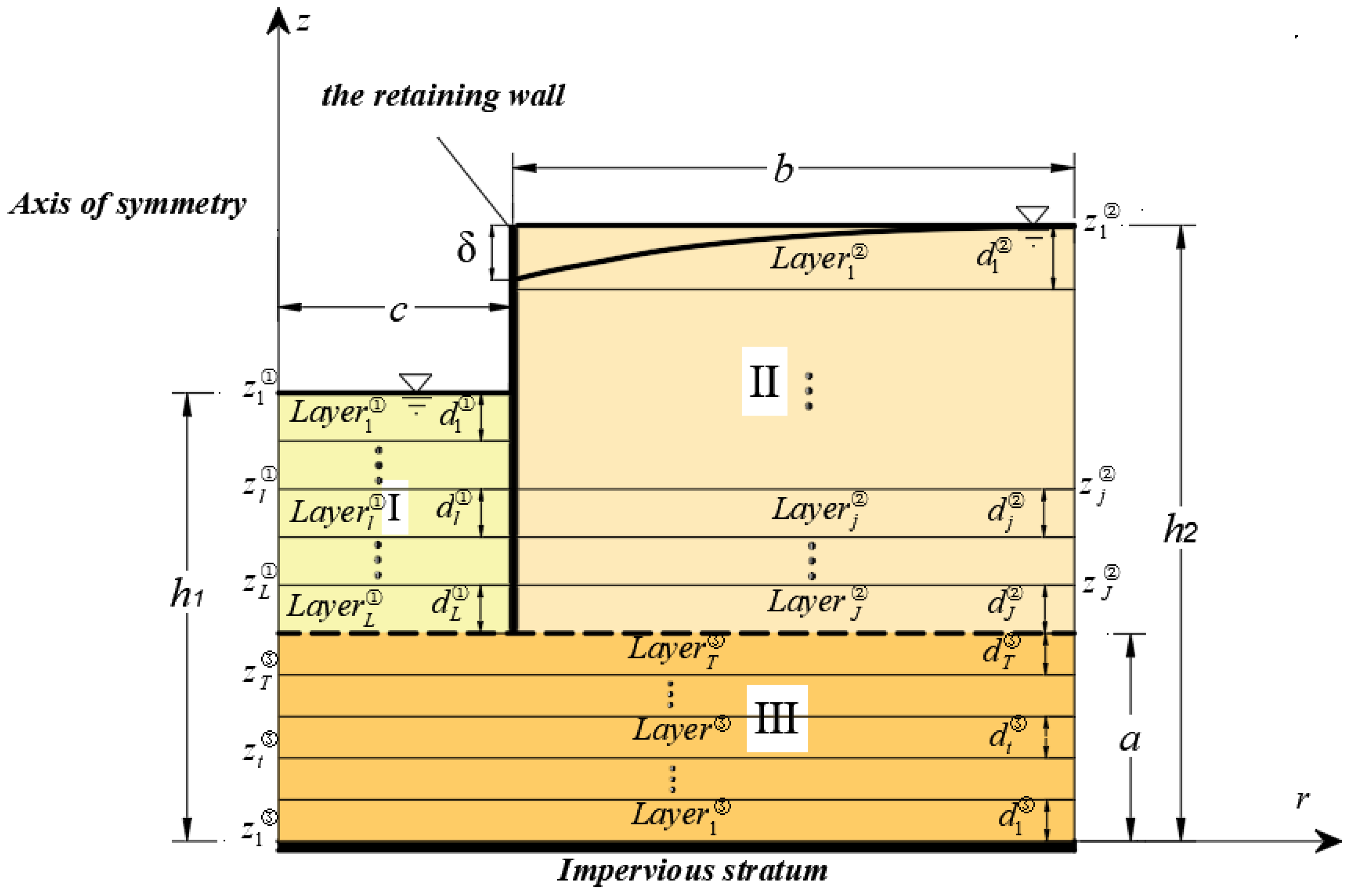
2.1. Proposal for Seepage Model of Anchor Circular Pit

The calculation model makes the following assumptions:

(1)

The seepage is in a stable state after the excavation and precipitation of the foundation pit.

(2)

The soil is incompressible, and the steady seepage is linear, in accordance with Darcy’s law.

(3)

The thickness of the retaining wall is ignored, and the effect of its contact with the soil on permeability is not considered.

(4)

The soil is assumed to be a layered non-homogeneous foundation. This means that each layer of soil is homogeneous and has an isotropic coefficient of permeability. The coefficients of permeability are different for each layer of soil.

(5)

The water recharge in the soil layer is mainly lateral, and vertical recharge can be ignored.

Due to the axisymmetric property of the foundation pit model, in order to simplify the calculation, the centerline of the foundation pit was taken as the axis to establish the two-dimensional seepage model of the foundation pit. The size of the model is shown in Figure 1. In the model, the distance between the bottom of the retaining wall and the top surface of the impervious layer is a, the outer width of the foundation pit is $b$, the half width of the foundation pit is c, the infinite distal water level on the outside of the foundation pit is $h_2$, and the inner water level is $h_1$, the flow domain was divided into three zones for mathematical convenience, the permeability coefficients of the layered soil layer, denoted by $k_l$, $k_j$ and $k_t$, respectively (l = 1 to L, j = 1 to J, and t = 1 to T), were constant in Zone Ⅰ, Ⅱ, and Ⅲ.

2.2. Governing Equations and Boundary Conditions

As shown in Figure 1, the seepage field of the foundation pit can be divided into Zone Ⅰ, Zone Ⅱ, and Zone Ⅲ based on the horizontal line of the retaining wall and the bottom wall. Assuming that the seepage in the soil satisfies Darcy’s law Cong (2009) [9], the seepage of layered soil in Zone Ⅰ, Zone Ⅱ, and Zone Ⅲ satisfies the equilibrium equation as follows:

$$\frac{1}{r}\frac{\partial }{\partial r}(r\times \frac{\partial H_l}{\partial r})+\frac{{\partial }^2{H}_l}{\partial z^2}=0;l=1,2,3,\cdot \cdot \cdot ,L$$

(1)

$$\frac{1}{r}\frac{\partial }{\partial r}(r\times \frac{\partial H_j}{\partial r})+\frac{{\partial }^2{H}_j}{\partial z^2}=0;j=1,2,3,\cdot \cdot \cdot ,J$$

(2)

$$\frac{1}{r}\frac{\partial }{\partial r}(r\times \frac{\partial H_t}{\partial r})+\frac{{\partial }^2{H}_t}{\partial z^2}=0;t=1,2,3,\cdot \cdot \cdot ,T$$

(3)

where $H_l$, $H_j$, and $H_t$ are the total hydraulic head distribution functions of layered soil in Zones Ⅰ, Ⅱ, and Ⅲ, respectively, the base level of the head calculation is the soil base level.

Since the upper boundary of region II is the submerged surface boundary, it is a special boundary with uncertain location. Based on the seepage theory by Bear J (1988) [10] it is known that the submerged surface conditions under isotropic soil conditions are as follows:

$$H(r,z,t)=z$$

(4)

$$K{(\frac{\partial H}{\partial r})}^2-K\frac{\partial H}{\partial z}+W={\mu }_d\frac{\partial H}{\partial t}$$

(5)

where K is the permeability coefficient, W is the upper recharge volume, and μ_d is the effective recharge degree of the aquifer.

Since Equation (5) is a non-linear equation, it is very difficult to satisfy Equations (4) and (5) simultaneously. This paper studies a pit in steady-state seepage situation. And the water recharge of the pit mainly comes from the infinite distal end. The upper recharge is small and can be neglected. Therefore, $\partial H/\partial t=0$, W = 0.

As for ${(\partial H/\partial r)}^2$, it is a higher-order infinitesimal term, which can be ignored in the solution.

$${(\partial H/\partial r)}^2\to 0$$

(6)

In addition, the height of the submerged surface drop, $\delta$, is generally small compared to the initial thickness of the aquifer. In summary, Equation (3) can be approximated as satisfying the following equation at z = h₁ Neuman (1974) [11]:

$${\frac{\partial H}{\partial z}|}_{z=h_1}=0$$

(7)

Equation (6) is the seepage boundary condition for the infiltration line in Zone II. Combined with the basic assumption of two-dimensional seepage in a foundation pit and the continuous conditions of layered soil in the subregion, the boundary and interfacial conditions of Zone Ⅰ can be obtained as follows:

$$H_l=h_1,\hspace{1em}0<r<c,\hspace{1em}z=z_{1\hspace{0.17em}0}=h_1\hspace{1em}$$

(8)

$$\frac{\partial H_l}{\partial r}=0,\hspace{1em}r=c,\hspace{1em}a<z<h_1$$

(9)

$$H_l=H_{\hspace{0.17em}l-1},0<r<c,\hspace{1em}z=z_{l-1}$$

(10)

$$k_l\frac{\partial H_l}{\partial z}=k_{l-1}\frac{\partial H_{l-1}}{\partial z},\hspace{1em}0<r<c,\hspace{1em}z=z_{l-1}$$

(11)

where $z_l$ is the distance from the impervious barrier to the upper interface of the l-th soil layer in Zone I, written as follows:

$$z_l=h_1-{\displaystyle \sum _{l=1}^{l-1}{d}_l^{②}=h_1-\left(d_1^{②}+d_2^{②}+\cdots +d_l^{②}\right)},\hspace{1em}l=1,2,\cdots ,L$$

(12)

Then the boundary and interfacial conditions of Zone Ⅱ can be obtained as follows:

$$\frac{\partial H_j}{\partial z}=0,\hspace{1em}c<r<b+c,\hspace{1em}z=z_{2\hspace{0.17em}0}=h_2\hspace{1em}$$

(13)

$$\frac{\partial H_j}{\partial r}=0,\hspace{1em}r=c,\hspace{1em}a<z<h_2$$

(14)

$$H_j=h_2,\hspace{1em}r=b+\mathrm{c},\hspace{1em}a<z<h_2$$

(15)

$$H_j=H_{j-1},\hspace{1em}c<r<b+c,\hspace{1em}z=z_{j-1}$$

(16)

$$k_j\frac{\partial H_j}{\partial z}=k_{j-1}\frac{\partial H_{j-1}}{\partial z},\hspace{1em}c<r<b+c,\hspace{1em}z=z_{j-1}$$

(17)

where $z_j$ is the distance from the impervious barrier to the upper interface of the j-th soil layer in Zone I, written as follows:

$$z_{\hspace{0.17em}j}=h_2-{\displaystyle \sum _{j=1}^{j-1}{d}_j^{②}=h_2-\left(d_1^{②}+d_2^{②}+\cdots +d_j^{②}\right)},\hspace{1em}j=1,2,\cdots ,J$$

(18)

The boundary and interfacial conditions of Zone Ⅲ can be obtained as follows:

$$\frac{\partial H_t}{\partial z}=0,\hspace{1em}0<r<b+c,\hspace{1em}z=z_{3\hspace{0.17em}0}=0\hspace{1em}$$

(19)

$$H_t=h_2,\hspace{1em}r=b+c,\hspace{1em}0<z<a$$

(20)

$$H_{\hspace{0.17em}t}=H_{t-1},\hspace{1em}0<r<b+c,\hspace{1em}z=z_{t-1}$$

(21)

$$k_{\hspace{0.17em}\hspace{0.17em}t}\frac{\partial H_t}{\partial z}=k_{t-1}\frac{\partial H_{t-1}}{\partial z},\hspace{1em}0<r<b+c,\hspace{1em}z=z_{t-1}$$

(22)

where $z_t$ is the distance from the impervious barrier to the lower interface of the t-th soil layer in Zone Ⅲ, written as follows:

$$z_t={\displaystyle \sum _{t=1}^{t-1}{d}_t^{②}=d_1^{②}+d_2^{②}+\cdots +d_t^{②}},\hspace{1em}t=1,2,\cdots ,T$$

(23)

For Zones Ⅰ and Ⅲ (between layer L and layer T),

$$H_L=H_T,\hspace{1em}0<r<c,\hspace{1em}z=z_L=z_T$$

(24)

$$k_L\frac{\partial H_L}{\partial z}=k_T\frac{\partial H_T}{\partial z},\hspace{1em}0<r<c,\hspace{1em}z=z_L=z_T$$

(25)

For Zones Ⅱ and Ⅲ (between layer J and layer T),

$$H_J=H_T,\hspace{1em}c<r<b+c,\hspace{1em}z=z_J=z_T$$

(26)

$$k_J\frac{\partial H_J}{\partial z}=k_{\hspace{0.17em}T}\frac{\partial H_T}{\partial z},\hspace{1em}c<r<b+c,\hspace{1em}z=z_{\hspace{0.17em}J}=z_{\hspace{0.17em}T}$$

(27)

3. Analytical Solution

3.1. Solution for the Hydraulic Head

Calling upon the separation of variable technique Yu (2023) [12], the total water heads of the layered soil in Zones Ⅰ, Ⅱ, and Ⅲ can be written in the form of a series sum as follows:

For Zone Ⅰ,

$$H_l\left(r,z\right)=\{\begin{array}{l}{h}_1+D_l\left(z-h_1\right)+{\displaystyle \sum _{n=1}^{\infty }{D}_{n\hspace{0.17em}l}\sinh {\lambda }_n\left(z-h_1\right)}{J}_0({\lambda }_{n}r) (l=1)\\ D_{l}z+E_l+{\displaystyle \sum _{n=1}^{\infty }\left(D_{n\hspace{0.17em}l}\cosh {\lambda }_{n}z+E_{n\hspace{0.17em}l}\sinh {\lambda }_{n}z\right)}{J}_0({\lambda }_{n}r) (l\ge 2)\end{array}$$

(28)

where ${\lambda }_n$ are roots of the following equation:

$$J_1({\lambda }_{n}c)=0$$

(29)

For Zone Ⅱ,

$$H_j\left(r,z\right)=\{\begin{array}{l}{h}_2+{\displaystyle \sum _{m=1}^{\infty }{F}_{m\hspace{0.17em}j}\cosh {\lambda }_m\left(z-h_2\right)}(J_0({\lambda }_{m}r)-\frac{J_1({\lambda }_{m}c)}{Y_1({\lambda }_{m}c)}\cdot Y_0({\lambda }_{m}r)) (j=1)\\ h_2+{\displaystyle \sum _{m=1}^{\infty }\left(F_{m\hspace{0.17em}j}\cosh {\lambda }_{m}z+G_{m\hspace{0.17em}j}\sinh {\lambda }_{m}z\right)}(J_0({\lambda }_{m}r)-\frac{J_1({\lambda }_{m}c)}{Y_1({\lambda }_{m}c)}\cdot Y_0({\lambda }_{m}r)) (j\ge 2)\end{array}$$

(30)

where ${\lambda }_m$ are roots of the following equation:

$$\left|\begin{array}{cc}{J}_1({\lambda }_{m}c)& Y_1({\lambda }_{m}c)\\ J_0[{\lambda }_m(b+c)]& Y_0[{\lambda }_m(b+c)]\end{array}\right|=0$$

(31)

For Zone Ⅲ,

$$H_t\left(r,z\right)=\{\begin{array}{l}{h}_2+{\displaystyle \sum _{i=1}^{\infty }{U}_{i\hspace{0.17em}t}}\cosh {\lambda }_{i}z{J}_0({\lambda }_{i}r) (t=1)\\ h_2+{\displaystyle \sum _{i=1}^{\infty }\left(U_{i\hspace{0.17em}t}\cosh {\lambda }_{i}z+K_{i\hspace{0.17em}t}\sinh {\lambda }_{i}z\right)}{J}_0({\lambda }_{i}r) (t\ge 2)\end{array}$$

(32)

where ${\lambda }_i$ are roots of the following equation:

$$J_0({\lambda }_{i}c)=0$$

(33)

The $H_l$ of Equations (28) and (29) satisfies the boundary conditions in Equations (8)–(10), and $H_t$ of Equations (32) and (33) satisfies Equations (19)–(21), by their very definition. Utilizing the interfacial conditions of layered soil in Zones Ⅰ, Ⅱ, and Ⅲ, respectively, and the regional interface z = a to evaluate the undetermined coefficients $D_l$, $E_l$, $D_{nl}$, $E_{nl}$, $F_{mj}$, $G_{mj}$, $U_{it}$, and $K_{it}$ appearing in the expressions of total water head functions $H_l$, $H_j$, and $H_t$ are proposed.

Applying the interfacial conditions in Equations (10) and (11) to Equation (28) for $H_l$ in Zone Ⅰ as follows be

$$\begin{array}{l}{D}_l{z}_{l-1}+E_l+{\displaystyle \sum _{n=1}^{\infty }\left(D_{nl}\cosh {\lambda }_n{z}_{l-1}+E_{nl}\sinh {\lambda }_n{z}_{l-1}\right)}{J}_0({\lambda }_{n}r)\\ \hspace{1em}\hspace{1em}\hspace{1em}\hspace{1em}\hspace{1em}=h_1+D_{1\hspace{0.17em}1}\left(z_{l-1}-h_1\right)+{\displaystyle \sum _{n=1}^{\infty }{D}_{n\hspace{0.17em}(l-1)}\sinh {\lambda }_n\left(z_{l-1}-h_1\right)}{J}_0({\lambda }_{n}r)\end{array}$$

(34)

$$\begin{array}{l}{D}_l+{\displaystyle \sum _{n=1}^{\infty }{\lambda }_n\left(D_{n\hspace{0.17em}l}\sinh {\lambda }_n{z}_{l-1}+E_{n\hspace{0.17em}l}\cosh {\lambda }_n{z}_{l-1}\right)}{J}_0({\lambda }_{n}r)\\ \hspace{1em}\hspace{1em}\hspace{1em}=\frac{k_{l-1}}{k_l}\left[D_{l-1}+{\displaystyle \sum _{n=1}^{\infty }{D}_{n\hspace{0.17em}(l-1)}{\lambda }_n\cosh {\lambda }_n\left(z_{l-1}-h_1\right)}{J}_0({\lambda }_{n}r)\right]\end{array}$$

(35)

$$\begin{array}{l}{D}_{\hspace{0.17em}l}{z}_{l-1}+E_l+{\displaystyle \sum _{n=1}^{\infty }\left(D_{n\hspace{0.17em}l}\cosh {\lambda }_n{z}_{l-1}+E_{n\hspace{0.17em}l}\sinh {\lambda }_n{z}_{l-1}\right)}{J}_0({\lambda }_{n}r)\\ \hspace{1em}\hspace{1em}\hspace{1em}\hspace{1em}\hspace{1em}\hspace{1em}=D_{l-1}{z}_{l-1}+E_{l-1}+{\displaystyle \sum _{n=1}^{\infty }\left(D_{n\hspace{0.17em}(l-1)}\cosh {\lambda }_n{z}_{l-1}+E_{n(\hspace{0.17em}l-1)}\sinh {\lambda }_n{z}_{l-1}\right)}{J}_0({\lambda }_{n}r)\end{array}$$

(36)

$$\begin{array}{l}{D}_l+{\displaystyle \sum _{n=1}^{\infty }{\lambda }_n\left(D_{n\hspace{0.17em}l}\sinh {\lambda }_n{z}_{l-1}+E_{n\hspace{0.17em}l}\cosh {\lambda }_n{z}_{l-1}\right)}{J}_0({\lambda }_{n}r)\\ \hspace{1em}\hspace{1em}\hspace{1em}\hspace{1em}\hspace{1em}\hspace{1em}=\frac{k_{l-1}}{k_{\hspace{0.17em}l}}\left[D_{l-1}+{\displaystyle \sum _{n=1}^{\infty }{\lambda }_n\left(D_{n(\hspace{0.17em}l-1)}\sinh {\lambda }_n{z}_{l-1}+E_{n(\hspace{0.17em}l-1)}\cosh {\lambda }_n{z}_{l-1}\right)}{J}_0({\lambda }_{n}r)\right]\end{array}$$

(37)

In the previous equations, the constants $E_l$ and $E_{nl}$ can be expressed linearly using $D_l$, $h_1$, and $D_{nl}$, respectively; the relevant expression for the same can be written as follows:

$$E_l=h_1+D_l{\alpha }_l$$

(38)

$$E_{nl}={\alpha }_{nl}\cdot D_{nl}$$

(39)

$$D_{nl}=\{\begin{array}{l}\frac{D_{n\hspace{0.17em}(l-1)}\sinh {\lambda }_n\left(z_{l-1}-h_1\right)}{\cosh {\lambda }_n{z}_{l-1}+{\alpha }_{n\hspace{0.17em}(l-1)}\sinh {\lambda }_n{z}_{l-1}} , l=2\\ D_{n(l-1)}\frac{\cosh {\lambda }_n{z}_{l-1}+{\alpha }_{n\hspace{0.17em}(l-1)}\sinh {\lambda }_n{z}_{l-1}}{\cosh {\lambda }_n{z}_{l-1}+{\alpha }_{n\hspace{0.17em}(l-1)}\sinh {\lambda }_n{z}_{l-1}} , l\ge 3\end{array}$$

(40)

Applying the linear correlation in Equations (38) and (39) to Equations (34)–(37), the correlation coefficients ${\alpha }_l$ and ${\alpha }_{nl}$ are obtained by carrying out a Fourier series expression in the domain 0 < r < c as follows:

$${\alpha }_l=\{\begin{array}{l}\frac{k_l}{k_{l-1}}\left(z_{l-1}-h_1\right)-z_{l-1} , l=2\\ \frac{k_l}{k_{l-1}}\left(z_{l-1}+{\alpha }_{l-1}\right)-z_{l-1} , l\ge 3\end{array}$$

(41)

$${\alpha }_{n\hspace{0.17em}l}=\{\begin{array}{l}\frac{\sinh {\lambda }_n{z}_{l-1}\cdot \tanh {\lambda }_n\left(z_{l-1}-h_1\right)-\frac{k_{l-1}}{k_{\hspace{0.17em}l}}\cosh {\lambda }_n{z}_{l-1}}{-\cosh {\lambda }_n{z}_{l-1}\cdot \tanh {\lambda }_n\left(z_{l-1}-h_1\right)+\frac{k_{l-1}}{k_{\hspace{0.17em}l}}\sinh {\lambda }_n{z}_{l-1}}l=2\\ \\ \frac{\sinh {\lambda }_n{z}_{l-1}\cdot \frac{\cosh {\lambda }_n{z}_{l-1}+\sinh {\lambda }_n{z}_{l-1}\cdot {\alpha }_{n\hspace{0.17em}(l-1)}}{\frac{k_{l-1}}{k_{\hspace{0.17em}l}}\left(\sinh {\lambda }_n{z}_{l-1}+\cosh {\lambda }_n{z}_{l-1}\cdot {\alpha }_{n\hspace{0.17em}(l-1)}\right)}-\cosh {\lambda }_n{z}_{l-1}}{\sinh {\lambda }_n{z}_{l-1}-\cosh {\lambda }_n{z}_{l-1}\cdot \frac{\cosh {\lambda }_n{z}_{l-1}+\sinh {\lambda }_n{z}_{l-1}\cdot {\alpha }_{n\hspace{0.17em}(l-1)}}{\frac{k_{l-1}}{k_{\hspace{0.17em}l}}\left(\sinh {\lambda }_n{z}_{l-1}+\cosh {\lambda }_n{z}_{l-1}\cdot {\alpha }_{n\hspace{0.17em}(l-1)}\right)}}l\ge 3 \end{array}$$

(42)

Again, applying the interfacial conditions in Equations (16) and (17) to Equations (30) and (31) for $h_j$ in Zone Ⅱ, we obtain the following:

$$\begin{array}{l}{h}_2+{\displaystyle \sum _{m=1}^{\infty }\left(F_{m\hspace{0.17em}j}\cosh {\lambda }_m{z}_{j-1}+G_{m\hspace{0.17em}j}\sinh {\lambda }_m{z}_{j-1}\right)}(J_0({\lambda }_{m}r)-\frac{J_1({\lambda }_{m}c)}{Y_1({\lambda }_{m}c)}\cdot Y_0({\lambda }_{m}r))\\ \hspace{1em}\hspace{1em}\hspace{1em}\hspace{1em}\hspace{1em}=h_2+{\displaystyle \sum _{m=1}^{\infty }{F}_{m\hspace{0.17em}(j-1)}\cosh {\lambda }_m\left(z_{j-1}-h_2\right)}(J_0({\lambda }_{m}r)-\frac{J_1({\lambda }_{m}c)}{Y_1({\lambda }_{m}c)}\cdot Y_0({\lambda }_{m}r))\end{array}$$

(43)

$$\begin{array}{l}{\displaystyle \sum _{m=1}^{\infty }{\lambda }_m\left(F_{m\hspace{0.17em}j}\sinh {\lambda }_m{z}_{j-1}+G_{m\hspace{0.17em}j}\cosh {\lambda }_m{z}_{j-1}\right)}(J_0({\lambda }_{m}r)-\frac{J_1({\lambda }_{m}c)}{Y_1({\lambda }_{m}c)}\cdot Y_0({\lambda }_{m}r))\\ \hspace{1em}\hspace{1em}\hspace{1em}=\frac{k_{j-1}}{k_j}{\displaystyle \sum _{m=1}^{\infty }{F}_{m(j-1)}{\lambda }_m\sinh {\lambda }_m\left(z_{j-1}-h_2\right)}(J_0({\lambda }_{m}r)-\frac{J_1({\lambda }_{m}c)}{Y_1({\lambda }_{m}c)}\cdot Y_0({\lambda }_{m}r))\end{array}$$

(44)

$$\begin{array}{l}{h}_2+{\displaystyle \sum _{m=1}^{\infty }\left(F_{m\hspace{0.17em}(j-1)}\cosh {\lambda }_m{z}_{j-1}+G_{m\hspace{0.17em}(j-1)}\sinh {\lambda }_m{z}_{j-1}\right)}\left(J_0({\lambda }_{m}r)-\frac{J_1({\lambda }_{m}c)}{Y_1({\lambda }_{m}c)}\cdot Y_0({\lambda }_{m}r)\right)\\ \hspace{1em}\hspace{1em}\hspace{1em}\hspace{1em}\hspace{1em}\hspace{1em}=h_2+{\displaystyle \sum _{m=1}^{\infty }\left(F_{m\hspace{0.17em}j}\cosh {\lambda }_m{z}_{j-1}+G_{m\hspace{0.17em}j}\sinh {\lambda }_m{z}_{j-1}\right)}\left(J_0({\lambda }_{m}r)-\frac{J_1({\lambda }_{m}c)}{Y_1({\lambda }_{m}c)}\cdot Y_0({\lambda }_{m}r)\right)\end{array}$$

(45)

$$\begin{array}{l}{\displaystyle \sum _{m=1}^{\infty }{\lambda }_m\left(F_{m\hspace{0.17em}(j-1)}\sinh {\lambda }_m{z}_{j-1}+G_{m\hspace{0.17em}(j-1)}\cosh {\lambda }_m{z}_{j-1}\right)}\left(J_0({\lambda }_{m}r)-\frac{J_1({\lambda }_{m}c)}{Y_1({\lambda }_{m}c)}\cdot Y_0({\lambda }_{m}r)\right)\\ \hspace{1em}\hspace{1em}\hspace{1em}\hspace{1em}\hspace{1em}\hspace{1em}=\frac{k_j}{k_{j-1}}{\displaystyle \sum _{m=1}^{\infty }{\lambda }_m\left(F_{m\hspace{0.17em}j}\sinh {\lambda }_m{z}_{j-1}+G_{m\hspace{0.17em}j}\cosh {\lambda }_m{z}_{j-1}\right)}\left(J_0({\lambda }_{m}r)-\frac{J_1({\lambda }_{m}c)}{Y_1({\lambda }_{m}c)}\cdot Y_0({\lambda }_{m}r)\right)\end{array}$$

(46)

In the previous equations, the constants $G_{mj}$ can be expressed linearly using $F_{mj}$, respectively, the relevant expression for the same can be written as follows:

$$G_{m\hspace{0.17em}j}={\beta }_{m\hspace{0.17em}j}\cdot F_{m\hspace{0.17em}j}$$

(47)

$$F_{mj}=\{\begin{array}{l}{F}_{m(j-1)}\frac{\cosh {\lambda }_m\left(z_{j-1}-h_2\right)}{\cosh {\lambda }_m{z}_{j-1}+{\beta }_{m\hspace{0.17em}j}\sinh {\lambda }_m{z}_{j-1}} , j=2\\ F_{m(j-1)}\frac{\cosh {\lambda }_m{z}_{j-1}+{\beta }_{m(\hspace{0.17em}j-1)}\sinh {\lambda }_m{z}_{j-1}}{\cosh {\lambda }_m{z}_{j-1}+{\beta }_{m\hspace{0.17em}j}\sinh {\lambda }_m{z}_{j-1}} , j\ge 3\end{array}$$

(48)

Applying the linear correlation in Equations (47) and (48) to Equations (43)–(46), the correlation coefficients ${\beta }_{mj}$ are given as follows:

$${\beta }_{m\hspace{0.17em}j}=\{\begin{array}{l}\frac{\frac{k_{j-1}}{k_j}\cosh {\lambda }_m{z}_{j-1}\cdot \tanh {\lambda }_m\left(z_{j-1}-h_2\right)+\sinh {\lambda }_m{z}_{j-1}}{\cosh {\lambda }_m{z}_{j-1}-\frac{k_{j-1}}{k_j}\cosh {\lambda }_m{z}_{j-1}\cdot \tanh {\lambda }_m\left(z_{j-1}-h_2\right)}j=2 \\ \\ \frac{\sinh {\lambda }_m{z}_{j-1}\cdot \frac{\cosh {\lambda }_m{z}_{j-1}+\sinh {\lambda }_m{z}_{j-1}\cdot {\beta }_{m\hspace{0.17em}\hspace{0.17em}(j-1)}}{\frac{k_{j-1}}{k_j}\left(\sinh {\lambda }_m{z}_{j-1}+\cosh {\lambda }_m{z}_{j-1}\cdot {\beta }_{m\hspace{0.17em}\hspace{0.17em}(j-1)}\right)}-\cosh {\lambda }_m{z}_{j-1}}{\sinh {\lambda }_m{z}_{j-1}-\cosh {\lambda }_m{z}_{j-1}\cdot \frac{\cosh {\lambda }_m{z}_{j-1}+\sinh {\lambda }_m{z}_{j-1}\cdot {\beta }_{m\hspace{0.17em}\hspace{0.17em}(j-1)}}{\frac{k_{j-1}}{k_j}\left(\sinh {\lambda }_m{z}_{j-1}+\cosh {\lambda }_m{z}_{j-1}\cdot {\beta }_{m\hspace{0.17em}\hspace{0.17em}(j-1)}\right)}}j>2\end{array}$$

(49)

Then, the interfacial conditions in Equations (21) and (22) are applied to Equations (32) and (33) for $h_t$ in Zone Ⅲ as follows:

$$\begin{array}{l} h_2+{\displaystyle \sum _{i=1}^{\infty }\left(U_{i\hspace{0.17em}t}\cosh {\lambda }_i{z}_{t-1}+K_{i\hspace{0.17em}t}\sinh {\lambda }_i{z}_{t-1}\right)}{J}_0({\lambda }_{i}r)\\ =h_2+{\displaystyle \sum _{i=1}^{\infty }{U}_{i\hspace{0.17em}(t-1)}}\cosh {\lambda }_i{z}_{t-1}{J}_0({\lambda }_{i}r)\end{array}$$

(50)

$$\begin{array}{l}{\displaystyle \sum _{i=1}^{\infty }{\lambda }_i{k}_t\left(U_{i\hspace{0.17em}t}\cosh {\lambda }_{i}z+K_{i\hspace{0.17em}t}\sinh {\lambda }_{i}z\right)}{J}_0({\lambda }_{i}r)\\ ={\lambda }_i{k}_{t-1}{\displaystyle \sum _{i=1}^{\infty }{U}_{i\hspace{0.17em}(t-1)}}\cosh {\lambda }_{i}z{J}_0({\lambda }_{i}r)\end{array}$$

(51)

$$\begin{array}{l} h_2+{\displaystyle \sum _{i=1}^{\infty }\left(U_{i\hspace{0.17em}t}\cosh {\lambda }_i{z}_{t-1}+K_{i\hspace{0.17em}t}\sinh {\lambda }_i{z}_{t-1}\right)}{J}_0({\lambda }_{i}r)\\ =h_2+{\displaystyle \sum _{i=1}^{\infty }\left(U_{i\hspace{0.17em}(t-1)}\cosh {\lambda }_i{z}_{t-1}+K_{i\hspace{0.17em}(t-1)}\sinh {\lambda }_i{z}_{t-1}\right)}{J}_0({\lambda }_{i}r)\end{array}$$

(52)

$$\begin{array}{l}{k}_t{\displaystyle \sum _{i=1}^{\infty }{\lambda }_i\left(U_{i\hspace{0.17em}t}\cosh {\lambda }_i{z}_{t-1}+K_{i\hspace{0.17em}t}\sinh {\lambda }_i{z}_{t-1}\right)}{J}_0({\lambda }_{i}r)\\ =k_{t-1}{\displaystyle \sum _{i=1}^{\infty }{\lambda }_i\left(U_{i\hspace{0.17em}(t-1)}\sinh {\lambda }_i{z}_{t-1}+K_{i\hspace{0.17em}(t-1)}\cosh {\lambda }_i{z}_{t-1}\right)}{J}_0({\lambda }_{i}r)\end{array}$$

(53)

By making the constant and function level terms on both sides Equations (50)–(53) correspondingly equal, the following linear relationship can be introduced:

$$K_{i\hspace{0.17em}t}={\chi }_{i\hspace{0.17em}t}\cdot U_{i\hspace{0.17em}t}$$

(54)

$$U_{it}=\{\begin{array}{l}\frac{U_{i\hspace{0.17em}(t-1)}\cosh {\lambda }_i{z}_{t-1}}{\cosh {\lambda }_i{z}_{t-1}+{\chi }_{i\hspace{0.17em}t}\sinh {\lambda }_i{z}_{t-1}} (t=2)\\ U_{i\hspace{0.17em}(t-1)}\frac{\cosh {\lambda }_i{z}_{t-1}+{\chi }_{i\hspace{0.17em}(t-1)}\sinh {\lambda }_i{z}_{t-1}}{\cosh {\lambda }_i{z}_{t-1}+{\chi }_{it}\sinh {\lambda }_i{z}_{t-1}} (t>2)\end{array}$$

(55)

with

$${\chi }_{i\hspace{0.17em}t}=\{\begin{array}{l}\frac{\frac{k_{\hspace{0.17em}t-1}}{k_t}\cosh k_i{z}_{t-1}\cdot \tanh k_i{z}_{t-1}-\sinh k_i{z}_{t-1}}{\cosh k_i{z}_{t-1}-\frac{k_{\hspace{0.17em}t-1}}{k_t}\sinh k_i{z}_{t-1}\cdot \tanh k_i{z}_{t-1}} (t=2) \\ \\ \frac{\sinh {\lambda }_i{z}_{t-1}\cdot \frac{\cosh {\lambda }_i{z}_{t-1}+\sinh {\lambda }_i{z}_{t-1}\cdot {\chi }_{i\hspace{0.17em}t-1}}{\frac{k_{\hspace{0.17em}t-1}}{k_t}\left(\sinh {\lambda }_i{z}_{t-1}+\cosh {\lambda }_i{z}_{t-1}\cdot {\chi }_{i\hspace{0.17em}t-1}\right)}-\cosh {\lambda }_i{z}_{t-1}}{\sinh {\lambda }_i{z}_{t-1}-\cosh {\lambda }_i{z}_{t-1}\cdot \frac{\cosh {\lambda }_i{z}_{t-1}+\sinh {\lambda }_i{z}_{t-1}\cdot {\chi }_{i\hspace{0.17em}\hspace{0.17em}t-1}}{\frac{k_{\hspace{0.17em}t-1}}{k_t}\left(\sinh {\lambda }_i{z}_{t-1}+\cosh {\lambda }_i{z}_{t-1}\cdot {\chi }_{i\hspace{0.17em}t-1}\right)}} (t>2)\end{array}$$

(56)

Applying the continuous seepage conditions in Equations (28) and (33) to Equations (24) and (26), the relationship between the constants can be written into the following:

$$h_2+{\displaystyle \sum _{i=1}^{\infty }{U}_{i\hspace{0.17em}T}\left(\cosh {\lambda }_{i}a+{\chi }_{i\hspace{0.17em}T}\sinh {\lambda }_{i}a\right)}{J}_0({\lambda }_{i}r)$$

(57)

$$=\{\begin{array}{l}{D}_{L}z+E_L+{\displaystyle \sum _{n=1}^{\infty }{D}_{n\hspace{0.17em}L}\left(\cosh {\lambda }_{n}a+{\alpha }_{n\hspace{0.17em}L}\sinh {\lambda }_{n}a\right)}{J}_0({\lambda }_{n}r) (0\le r\le c)\\ h_2+{\displaystyle \sum _{m=1}^{\infty }{F}_{m\hspace{0.17em}J}\left(\cosh {\lambda }_{m}a+{\beta }_{m\hspace{0.17em}J}\sinh {\lambda }_{m}a\right)}(J_0({\lambda }_{m}r)-\frac{J_1({\lambda }_{m}c)}{Y_1({\lambda }_{m}c)}\cdot Y_0({\lambda }_{m}r)) (c\le r\le b+c)\end{array}$$

(58)

Again, applying the continuous seepage conditions in Equations (28)–(33) to Equations (25) and (27), the relationship between the constants is given as follows:

$${\displaystyle \sum _{i=1}^{\infty }{U}_{i\hspace{0.17em}T}{\lambda }_i\left(\sinh {\lambda }_{i}a+{\chi }_{i\hspace{0.17em}T}\cosh {\lambda }_{i}a\right)}{J}_0({\lambda }_{i}r)$$

(59)

$$=\{\begin{array}{l}\frac{k_L}{k_T}(D_L+{\displaystyle \sum _{n=1}^{\infty }{D}_{n\hspace{0.17em}L}{\lambda }_n\left(\sinh {\lambda }_{n}a+{\alpha }_{n\hspace{0.17em}L}\cosh {\lambda }_{n}a\right)}{J}_0({\lambda }_{n}r)) (0\le r\le c)\\ \frac{k_J}{k_T}{\displaystyle \sum _{m=1}^{\infty }{F}_{m\hspace{0.17em}J}{\lambda }_m\left(\sinh {\lambda }_{m}a+{\beta }_{m\hspace{0.17em}J}\cosh {\lambda }_{m}a\right)}(J_0({\lambda }_{m}r)-\frac{J_1({\lambda }_{m}c)}{Y_1({\lambda }_{m}c)}\cdot Y_0({\lambda }_{m}r)) (c\le r\le b+c)\end{array}$$

(60)

From Equations (57) and (60), the constant terms $D_L$$E_L$, and $U_{iT}$ are determined with the integral property of the Bessel function Zhang (2014) [13], as follows:

$$D_L=\frac{2}{c}\frac{k_T}{k_L}{\displaystyle \sum _{i=1}^{\infty }{U}_{iT}\left(\sinh {\lambda }_{i}a+{\chi }_{i\hspace{0.17em}T}\cdot \cosh {\lambda }_{i}a\right)}{J}_1({\lambda }_{i}c)$$

(61)

$$h_2=D_{L}a+E_L$$

(62)

For the seepage problem of layered soil, there still remain the constants $D_{nL}$, $F_{mJ}$, and $U_{iT}$ to be determined. To evaluate $D_{nL}$, multiplying both sides of Equation (59) by $r{J}_0({\lambda }_{n}r)$ and integrating within the intervals (0, c) yields, for ${\lambda }_n\ne {\lambda }_i$, the following:

$$\begin{array}{l}{\displaystyle \sum _{n=1}^{\infty }{D}_{n\hspace{0.17em}L}{\lambda }_n\left(\sinh {\lambda }_{n}a+{\alpha }_{n\hspace{0.17em}L}\cdot \cosh {\lambda }_{n}a\right)\frac{c^2}{2}{J}_0^2({\lambda }_{n}c)}\\ -{\displaystyle \sum _{i=1}^{\infty }\frac{k_{\hspace{0.17em}T}}{k_{\hspace{0.17em}L}}{\lambda }_i{U}_{i\hspace{0.17em}T}}\left(\sinh {\lambda }_{i}a+{\chi }_{i\hspace{0.17em}T}\cdot \cosh {\lambda }_{i}a\right)J_1({\lambda }_{i}c)J_0[{\lambda }_i(b+c)]\frac{c{\lambda }_i}{{\lambda }_i^2-{\lambda }_n^2}=0\end{array}$$

(63)

and, for ${\lambda }_n={\lambda }_i$, the following:

$$\begin{array}{l}{\displaystyle \sum _{n=1}^{\infty }{D}_{n\hspace{0.17em}L}{\lambda }_n\left(\sinh {\lambda }_{n}a+{\alpha }_{n\hspace{0.17em}L}\cdot \cosh {\lambda }_{n}a\right)\frac{c^2}{2}{J}_0^2({\lambda }_{n}c})\\ -{\displaystyle \sum _{i=1}^{\infty }\frac{k_{\hspace{0.17em}T}}{k_{\hspace{0.17em}L}}{\lambda }_i{U}_{i\hspace{0.17em}T}}\left(\sinh {\lambda }_{i}a+{\chi }_{i\hspace{0.17em}T}\cdot \cosh {\lambda }_{i}a\right)\frac{c^2{J}_0{}^2[{\lambda }_i(b+c)]}{2}=0\end{array}$$

(64)

Next, to determine the constant $F_{mJ}$, multiplying both sides of Equation (60) by $r(J_0({\lambda }_{m}r)-\frac{J_1({\lambda }_m{r}_0)}{Y_1({\lambda }_m{r}_0)}{Y}_0({\lambda }_{m}r))$ and integrating within the intervals (c, b + c) yields, for ${\lambda }_m\ne {\lambda }_i$, the following:

$$\begin{array}{l}{\displaystyle \sum _{m=1}^{\infty }{F}_{m\hspace{0.17em}J}{\lambda }_m\left(\sinh {\lambda }_{m}a+{\beta }_{m\hspace{0.17em}J}\cdot \cosh {\lambda }_{m}a\right)\frac{2}{{\pi }^2{\lambda }_m{}^2}[\frac{1}{Y_0^2[{\lambda }_m(b+c)]}-\frac{1}{Y_1^2({\lambda }_{m}c)}]}\\ -{\displaystyle \sum _{i=1}^{\infty }\frac{k_T}{k_J}{\lambda }_i{U}_{i\hspace{0.17em}T}}\left(\sinh {\lambda }_{i}a+{\chi }_{i\hspace{0.17em}T}\cdot \cosh {\lambda }_{i}a\right)\frac{2{\lambda }_i{J}_1({\lambda }_{i}c)}{\pi {\lambda }_m({\lambda }_i{}^2-{\lambda }_m{}^2)Y_1({\lambda }_{i}c)}=0\end{array}$$

(65)

and, for $k_m=k_i$, the following:

$$\begin{array}{l}{\displaystyle \sum _{m=1}^{\infty }{F}_{mJ}{\lambda }_m\left(\sinh {\lambda }_{m}a+{\beta }_{m\hspace{0.17em}J}\cdot \cosh {\lambda }_{m}a\right)\frac{2}{{\pi }^2{\lambda }_m{}^2}[\frac{1}{Y_0^2[{\lambda }_m(b+c)]}-\frac{1}{Y_1^2({\lambda }_{m}c)}]}\\ -{\displaystyle \sum _{i=1}^{\infty }\frac{k_T}{k_J}{\lambda }_i{U}_{i\hspace{0.17em}T}}\left(\sinh {\lambda }_{i}a+{\chi }_{i\hspace{0.17em}T}\cdot \cosh {\lambda }_{i}a\right)\frac{J_0({\lambda }_{m}c)}{\pi {\lambda }_m{Y}_1({\lambda }_{m}c)}=0\end{array}$$

(66)

Finally, the constants $U_{iT}$ are evaluated by multiplying both sides of Equations (57) and (58) by $r{J}_0({\lambda }_{i}r)$ and integrating within the intervals (0, b + c); this gives the relations for the constants $U_{iT}$, for ${\lambda }_n\ne {\lambda }_i$, ${\lambda }_m\ne {\lambda }_i$, as follows:

$$\begin{array}{l}{D}_{\hspace{0.17em}L}\left(a+{\alpha }_L\right)\frac{c{J}_1{\lambda }_{i}c}{{\lambda }_i}+{\displaystyle \sum _{n=1}^{\infty }{D}_{n\hspace{0.17em}L}}\left(\cosh {\lambda }_{n}a+{\alpha }_{n\hspace{0.17em}J}\cdot \sinh {\lambda }_{n}a\right)J_1({\lambda }_{i}c)J_0({\lambda }_{n}c)\frac{c{\lambda }_i}{{\lambda }_i^2-{\lambda }_n^2}\\ +{\displaystyle \sum _{m=1}^{\infty }{F}_{m\hspace{0.17em}J}}\left(\cosh {\lambda }_{m}a+{\beta }_{m\hspace{0.17em}J}\cdot \sinh {\lambda }_{m}a\right)\frac{2{\lambda }_i{J}_1({\lambda }_{i}c)}{\pi {\lambda }_m({\lambda }_i{}^2-{\lambda }_m{}^2)Y_1({\lambda }_{m}c)}\\ -{\displaystyle \sum _{i=1}^{\infty }{U}_{i\hspace{0.17em}T}\left(\cosh {\lambda }_{i}a+{\chi }_{i\hspace{0.17em}T}\cdot \sinh {\lambda }_{i}a\right)\frac{{(b+c)}^2}{2}{J}_1^2[{\lambda }_i(b+c)}]\\ =(h_2-h_1)\frac{c{J}_1({\lambda }_{i}c)}{{\lambda }_i}\end{array}$$

(67)

for ${\lambda }_n\ne {\lambda }_i$, as follows:

$$\begin{array}{l}{D}_{\hspace{0.17em}L}\left(a+{\alpha }_L\right)\frac{c{J}_1({\lambda }_{i}c)}{{\lambda }_i}+{\displaystyle \sum _{n=1}^{\infty }{D}_{n\hspace{0.17em}L}}\left(\cosh {\lambda }_{n}a+{\alpha }_{n\hspace{0.17em}J}\cdot \sinh {\lambda }_{n}a\right)\frac{c^2{J}_0{}^2[{\lambda }_i(b+c)]}{2}\\ +{\displaystyle \sum _{m=1}^{\infty }{F}_{m\hspace{0.17em}J}}\left(\cosh {\lambda }_{m}a+{\beta }_{m\hspace{0.17em}J}\cdot \sinh {\lambda }_{m}a\right)\frac{2{\lambda }_i{J}_1({\lambda }_{i}c)}{\pi {\lambda }_m({\lambda }_i{}^2-{\lambda }_m{}^2)Y_1({\lambda }_{m}c)}\\ -{\displaystyle \sum _{i=1}^{\infty }{U}_{i\hspace{0.17em}T}\left(\cosh {\lambda }_{i}a+{\chi }_{i\hspace{0.17em}T}\cdot \sinh {\lambda }_{i}a\right)\frac{{(b+c)}^2}{2}{J}_1^2[{\lambda }_i(b+c)}]\\ =(h_2-h_1)\frac{c{J}_1({\lambda }_{i}c)}{{\lambda }_i}\end{array}$$

(68)

and, for ${\lambda }_m\ne {\lambda }_i$, as follows:

$$\begin{array}{l}{D}_{\hspace{0.17em}L}\left(a+{\alpha }_L\right)\frac{c{J}_1({\lambda }_{i}c)}{{\lambda }_i}+{\displaystyle \sum _{n=1}^{\infty }{D}_{n\hspace{0.17em}L}}\left(\cosh {\lambda }_{n}a+{\alpha }_{n\hspace{0.17em}J}\cdot \sinh {\lambda }_{n}a\right)J_1({\lambda }_{i}c)J_0({\lambda }_{n}c)\frac{c{\lambda }_i}{{\lambda }_i^2-{\lambda }_n^2}\\ +{\displaystyle \sum _{m=1}^{\infty }{F}_{m\hspace{0.17em}J}\left(\cosh {\lambda }_{m}a+{\beta }_{m\hspace{0.17em}J}\cdot \sinh {\lambda }_{m}a\right)\frac{J_0({\lambda }_{m}c)}{\pi {\lambda }_m{Y}_1({\lambda }_{m}c)}}\\ -{\displaystyle \sum _{i=1}^{\infty }{U}_{i\hspace{0.17em}T}\left(\cosh {\lambda }_{i}a+{\chi }_{i\hspace{0.17em}T}\cdot \sinh {\lambda }_{i}a\right)\frac{{(b+c)}^2}{2}{J}_1^2[{\lambda }_i(b+c)}]\\ =(h_2-h_1)\frac{c{J}_1({\lambda }_{i}c)}{{\lambda }_i}\end{array}$$

(69)

The equations related to $D_L$, $D_{nL}$, $F_{mJ}$, and $U_{iT}$ in Equation (61) and Equations (63)–(69) can be solved by constructing non-linear equations. Since the series in the equation is infinite, the series must be truncated at the N-th term. Otherwise, it is impossible to solve the undetermined coefficient. In the Appendix A, the system of non-chiral linear equations for determining the unknown coefficients is listed.

By solving the matrix above, $D_L$, $D_{nL}$, $F_{mJ}$, and $U_{iT}$ can be obtained. There are already explicit relations for $D_L$, $D_{nL}$, $F_{mJ}$, and $U_{iT}$ in Equations (38), (41) and (42), Equations (47) and (49), and Equations (54) and (56) to evaluate these constants for layered soil in Zones Ⅰ, Ⅱ, and Ⅲ. Thus, all the constants appearing in the water head functions $H_l$, $H_j$, and $H_t$ are determined, and hence, the total water head distribution inside and outside the foundation pit can be obtained.

With an increase in the number of series, N, the accuracy of the calculated value of the water head is also improved. It needs to be pointed out that, when using MATLAB to solve the matrix with double precision, when the order of the coefficient matrix EE increases, the condition number also becomes larger and larger. The MATLAB multiprecision calculation toolbox can be used to solve this problem.

3.2. Solution for the Exit Hydraulic Gradient

According to the definition of the hydraulic gradient Terzaghi et al. (1996) [14], the hydraulic gradient at any point of the excavation surface can be solved based on the analytical solution of the total hydraulic head as follows:

$$i_e=-\frac{\partial H_1}{\partial z}|{}_{z=h_1}=-(D_1+{\displaystyle \sum _{n=1}^{\infty }{\lambda }_n{D}_{n1}{J}_0({\lambda }_{n}r))}$$

(70)

where $H_1$ is the hydraulic head function of the first layer in Zone Ⅰ. A positive i_e value indicates upward seepage.

3.3. Solution for Seepage Quantities

The seepage quantities are a key parameter in the design of arbitrarily shaped weirs, and an accurate estimation of flow is essential. According to Darcy’s law, the 3D seepage quantities at the excavation surface of the cofferdam can be described as follows:

$$Q=S\upsilon =Ski$$

(71)

where Q is the seepage quantity (${\mathrm{m}}^3/\mathrm{d}$), S is the seepage cross-sectional area (${\mathrm{m}}^2$), $\upsilon$ is the flow rate ($\mathrm{m}/\mathrm{s}$), and i is the hydraulic gradient.

It is known that the distribution of hydraulic gradient values at the excavation face of the cofferdam is axisymmetric Shi C (2021) [15]. Therefore, the total seepage quantities at the excavation surface can be considered to be the superposition of the seepage quantities in any circular area centred on the z-axis, where the flow per unit circular area can be expressed as follows:

$$q_h=2\pi k_{1}irdr$$

(72)

The total seepage quantities at the excavation surface are obtained by integrating the function $q_h$ from 0 to r₀:

$$\begin{array}{c}Q=-{\displaystyle {\int }_0^{c}2\pi k_1}(D_1+{\displaystyle \sum _{n=1}^{\infty }{\lambda }_n}{D}_{n1}{J}_0({\lambda }_{n}r))rdr\\ =-\pi r_0^2{k}_1{D}_1\end{array}$$

(73)

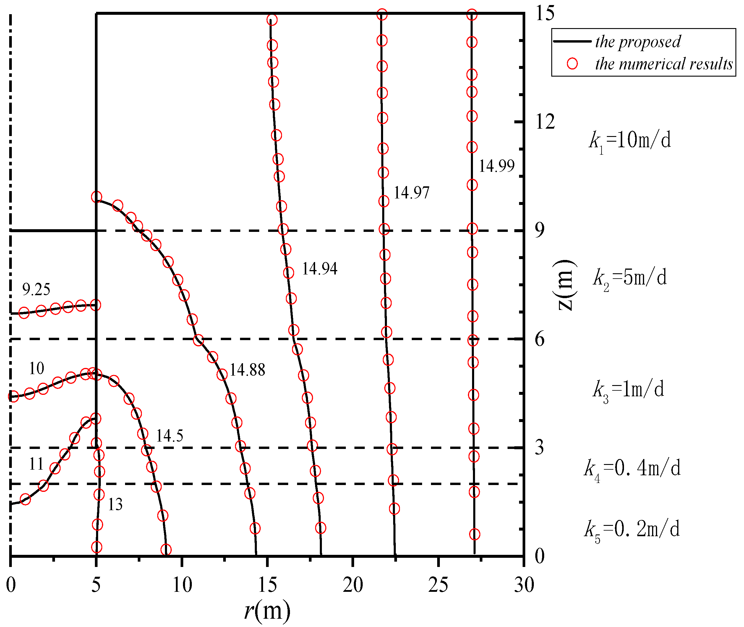
4. Verification of Proposed Solution

4.1. Verification of the Hydraulic Head Solution

To verify the correctness of the analytical solution in this paper, the numerical simulation was carried out using Plaxis 2D 8.5, a finite element numerical analysis software, and the numerical mesh was constructed with triangular elements. We assumed that there were five layers of soil with different permeability coefficients in the seepage field and the permeability coefficients of the soil layers were distributed from top to bottom as $k_1=1\times {10}^{-4} \mathrm{m}/\mathrm{s}$, $k_2=5\times {10}^{-5} \mathrm{m}/\mathrm{s}$, $k_3=1\times {10}^{-5} \mathrm{m}/\mathrm{s}$, $k_4=4\times {10}^{-6} \mathrm{m}/\mathrm{s}$, and $k_5=2\times {10}^{-6} \mathrm{m}/\mathrm{s}$, respectively.

Based on the analytical solution and the calculated results of the finite element software, the number of series terms, N = 60, was used to calculate the value of the seepage field near the two-dimensional foundation pit, as shown in Figure 2. The results of the analytical solution are consistent with the finite element calculation data, which verifies the accuracy of the analytical solution calculation.

4.2. Verification of Seepage in Excavation

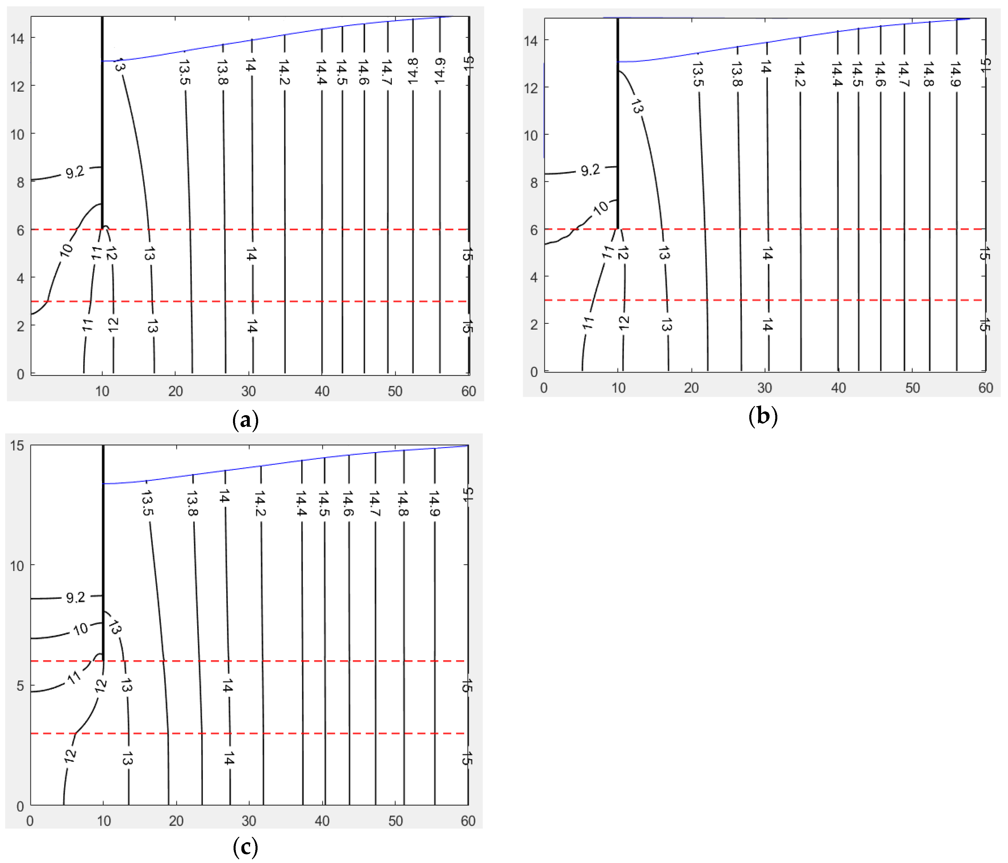
The example in Wang JH (2015) [8] was calculated with the seepage calculation, Formula (64), proposed in this paper. And the analytical solution calculation results were compared with the results of the modified large well method and the numerical calculation results. The specific calculation parameters were as follows: the radius of the pit was 50 m, and the depth of the basement was 7 m. The thickness of the aquifer was 60 m, the permeability coefficient was 150 m/d, and the radius of influence was 300 m. The depth of the groundwater level was 5 m, and the ground elevation was 40 m. The thickness of the cutoff wall D was set to 1 m. Keeping other parameters constant, the depth of the cutoff wall was increased from 10, 15, 20, 25, 30, 35, and 40 m to 45 m. The seepage quantity of the excavation for different depths of the cutoff wall was then calculated.

As can be seen in Figure 3, most of the relative errors between the modified large-well method and the numerical solution were within 10 percent. For the larger insertion depth of the cutoff wall, the local error between the modified large-well method and the numerical solution exceeded 20%. The calculated values of the analytical solution proposed in this paper were in better agreement with the numerical solution, and the errors were basically within 1.5%. And the error was not more than 2% for the larger insertion depth of the cutoff wall. This shows that the analytical solution of this paper can be used as a reliable tool for calculating the water inflow of a foundation pit.

5. Discussion

Consider the pit shown in Figure 4; the pit has three layers of soil, from top to bottom. The first layer of soil is 9 m thick, permeability coefficient is k₁. The second and third layers are 3 m thick, and their permeability coefficients are k₂ and k₃, respectively. The radius of the pit is 10 m, the far field distance of the pit is taken as 50 m, the distance of the retaining wall from the impermeable boundary at the bottom is 6 m, and the infinite distal head is 15 m. The effect of the permeability coefficient on the head distribution is then analyzed.

(1) Effect of change in the permeability coefficient, k₁, of the first soil layer on the seepage field

Plot the hydraulic head for three cases: $k_1=0.25 \mathrm{m}/\mathrm{d}$,$k_1=1 \mathrm{m}/\mathrm{d}$, and $k_1=4 \mathrm{m}/\mathrm{d}$, respectively. In the three cases, the coefficient of permeability of the second and third soil layers is constant, which is $k_2=k_3=1 \mathrm{m}/\mathrm{d}$. Through a comparison of Figure 5a–c, it can be found that, when the permeability coefficient k₁ decreases, by the pit diaphragm wall, the head at the same height in the gradual increases, whereas at the outside of the pit, the height of the free surface gradually decreases.

(2) Effect of change in the permeability coefficient, k₂, of the second soil layer on the seepage field

Plot the hydraulic head for three cases: $k_2=0.25 \mathrm{m}/\mathrm{d}$, $k_2=1 \mathrm{m}/\mathrm{d}$, and $k_2=4 \mathrm{m}/\mathrm{d}$, respectively. In the three cases, the coefficient of permeability of the second and third soil layers is constant, which is $k_1=k_3=1 \mathrm{m}/\mathrm{d}$. As can be seen from Figure 6a–c, with an increase in the permeability k₂, the head near the pit diaphragm at the same height increases inside the pit and decreases outside the pit; the height of the water table outside the pit also increases.

(3) Effect of change in the permeability coefficient, k₃, of the third soil layer on the seepage field

Plot the hydraulic head for three cases: $k_3=0.25 \mathrm{m}/\mathrm{d}$, $k_3=1 \mathrm{m}/\mathrm{d}$, and $k_3=4 \mathrm{m}/\mathrm{d}$, respectively. In the three cases, the coefficient of permeability of the second and third soil layers is constant, which is $k_1=k_2=1 \mathrm{m}/\mathrm{d}$. As can be seen from Figure 7, when the permeability coefficient of the soil layer changes suddenly, the head curve will also change at the soil layer boundary; with an increase in the permeability, k₃, the head near the pit diaphragm at the same height gradually increases within the pit as well as outside it, and the water level height outside the pit also increases.

As a result of the analyses of the three cases, it can be concluded that the ratio of the permeability coefficient between the soil layers is the key factor affecting the distribution of the seepage field. The larger the ratio of the permeability coefficient between the upper soil layer and the lower soil layer, taking the bottom of the retaining wall as the boundary, the larger the change in the head outside the pit and the larger the height of the water level drop.

6. Conclusions

In this paper, an analytical solution for steady-state seepage in anchor circular pits in homogeneous permeable isotropic soils is obtained. The analytical solution is obtained by solving the Laplacian using the separated variable method. The determination of the coefficients to be determined in the analytical solution makes use of the integral property of the Bessel function. According to the analytical solution, the infiltration line equation, the pit inrush volume, and the outlet hydraulic slope drop are further obtained, and the calculation results are compared with the numerical finite element results, etc. The following conclusions were finally obtained.

The analytical solution can calculate the hydraulic head value at any point of the seepage field of the circular pit, the hydraulic gradient of the excavation surface, the seepage volume, and the depth of the pit water level drop. The comparison with the numerical calculation results confirms the relevance of the analytical solution in this paper. In order to study the influence of the permeability coefficient on the distribution of the seepage field, the seepage field of the circular pit was analyzed by using a calculation example. The analysis results showed that the ratio of the permeability coefficients between soil layers was the key factor affecting the distribution of the seepage field.

Since the proposed solution for the foundation pit is for multilayered soil, in addition to the design of foundation pit parameters, the change in the conductivity of layered soil was also considered in the model. Therefore, the proposed solution is helpful to better analyze the seepage environment of a foundation pit. And, as mentioned above, since most of the soil in nature is naturally stratified, the study of a layered soil foundation pit seepage problem is closer to the reality, which provides an accurate basis for the construction and protection of foundation pits.

References

1. Navarro Carrasco, S.; Jiménez-Valera, J.A.; Alhama, I. A Universal Graphical Solution to Calculating Seepage in Excavation of Anisotropic Soils and Non-Limited Scenarios. Geotechnics 2023, 3, 719–730. [Google Scholar] [CrossRef]
2. Huang, D.-Z.; Xie, K.-H.; Ying, H.-W. Semi-analytical solution for two-dimensional steady seepage around foundation pit in soil layer with anisotropic permeability. J. Zheiiang Univ. (Eng. Sci.) 2014, 48, 1802–1808. [Google Scholar]
3. Fox, E.N.; Mcnamee, J., XXV. The two-dimensional potential problem of seepage into a cofferdam. J. Philos. Mag. 1948, 39, 165–203. [Google Scholar] [CrossRef]
4. Bereslavskii, E.N. The flow of ground waters around a Zhukovskii sheet pile. J. Appl. Math. Mech. 2011, 75, 210–217. [Google Scholar] [CrossRef]
5. Banerjee, S.; Muleshkov, A. Analytical solution of steady seepage into double-walled cofferdams. J. Eng. Mech. 1992, 118, 525–539. [Google Scholar] [CrossRef]
6. Chen, Z. Groundwater Flow Analysis of Confined Aquifer under Foundation Pit with Waterproof Curtain. Master’s Thesis, Nanjing Tech University, Nanjing, China, 2015. [Google Scholar]
7. Wang, J.H.; Tao, L.J.; Han, X. Effect of Suspended Curtain Depth into Stratum on Discharge Rate and Its Optimum Design. J. Beijing Univ. Technol. 2015, 41, 1390–1398. [Google Scholar]
8. Lin, Z.-b.; Li, Y.-m.; Gui, C.-i.; Liu, J.q.; Qin, X.-l. Method for steady flow of partially penetrating well in phreatic aquifer under constant flow. Chin. J. Geotech. Eng. 2013, 35, 2290–2297. [Google Scholar]
9. Cong, A.S. Discussion on several issues of seepage stability of deep foundation pit in multilayered formation. J. Chin. J. Rock Mech. Eng. 2009, 28, 2018–2023. [Google Scholar]
10. Bear, J. Dynamics of Fluids in Porous Media; American Elsevier Publishing Company: Amsterdam, The Netherlands, 1988. [Google Scholar]
11. Neuman, S.P. Effect of partial penetration on flow in unconfined aquifers considering delayed gravity response. Water Resour. Res. 1974, 10, 303–312. [Google Scholar] [CrossRef]
12. Yu, J.; Li, D.; Zheng, J.; Zhang, Z.; He, Z.; Fan, Y. Analytical study on the seepage field of different drainage and pressure relief options for tunnels in high water-rich areas. Tunn. Undergr. Space Technol. 2023, 134, 105018. [Google Scholar] [CrossRef]
13. Zhang, C. Anisotropic Mathematical Physics and Complex Special Functions; Scholastic Paperbacks: Beijing, China, 2014. [Google Scholar]
14. Terzaghi, K.; Peck, R.B.; Mesri, G. Soil Mechanics in Engineering Practice; Wiley: New York, NY, USA, 1996. [Google Scholar]
15. Shi, C.; Sun, X.; Liu, S.; Cao, C.; Liu, L.; Lei, M. Analysis of Seepage Characteristics of a Foundation Pit with Horizontal Waterproof Curtain in Highly Permeable Strata. Water 2021, 13, 1303. [Google Scholar] [CrossRef]
Figure 1. Model of two-dimensional seepage around anchor circular pit in layered soil.
Buildings 14 00074 g001
Figure 2. Two-dimensional contrast of water head distribution around anchor circular pit in layered soil.
Buildings 14 00074 g002
Figure 3. Comparison of seepage volume calculation results.
Buildings 14 00074 g003
Figure 4. Diagram of the pit parameters.
Buildings 14 00074 g004
Figure 5. Effect of change in permeability coefficient of the first layer of soil on head distribution. (a) k1 = 0.25 m/d; (b) k1 = 1 m/d; (c) k1 = 4 m/d.
Buildings 14 00074 g005
Figure 6. Influence of changes in the permeability coefficient of the second layer of soil on the distribution of the hydraulic head. (a) k1 = 0.25 m/d; (b) k1 = 1 m/d; (c) k1 = 4 m/d.
Buildings 14 00074 g006
Figure 7. Influence of changes in the coefficient of permeability of the third layer of soil on the head distribution. (a) k3 = 0.25 m/d; (b) k3 = 1 m/d; (c) k3 = 4 m/d.
Buildings 14 00074 g007
Disclaimer/Publisher’s Note: The statements, opinions and data contained in all publications are solely those of the individual author(s) and contributor(s) and not of MDPI and/or the editor(s). MDPI and/or the editor(s) disclaim responsibility for any injury to people or property resulting from any ideas, methods, instructions or products referred to in the content.