Theoretical Analysis of the Active Earth Pressure on Inclined Retaining Walls

Abstract

The estimation of earth pressure is crucial in the design of retaining structures. The evaluation of vertical retaining walls has been well studied within the framework of the differential flat element method in prior investigations, in which the vertical stress and maximum principal stress are assumed to be uniformly distributed. Inclined retaining walls have been successfully adopted in excavation engineering. Due to the inclination of retaining walls, the maximum principal stress direction rotates approximately parallel to the inclined wall back, which affects the active earth pressure on the walls. This paper provides an analytical solution to evaluate the active earth pressure on inclined retaining walls. A numerical model is first established to analyze the characteristics of the principal stresses and vertical stress distribution of soil behind walls with various inclination angles. An idealized vertical stress field containing two zones is developed, and a hyperbolic function is proposed to illustrate the distribution of vertical stress at various depths. Subsequently, the relationship between the nonuniform characteristics of the vertical stress and normal stress acting on a differential flat element is established based on a circular stress trajectory. The active earth pressure along the inclined wall is then obtained based on the balance of the forces on the differential elements. The predicted data from the proposed analytical solution are compared with the previous experimental, numerical, and theoretical results with excellent agreement, demonstrating the accuracy of the proposed method.

1. Introduction

Precise estimates of earth pressure are necessary for the design of retaining walls [1]. At present, the Rankine [2] and Coulomb [3] methods are widely used in engineering practice. Rankine [2] theory is derived by solving the soil limit equilibrium of each individual element to obtain the earth pressure, which considers the stress state of the retained soil behind retaining walls. Rankine theory is only applicable to a smooth and vertical wall, and the earth pressure is assumed to have a linear distribution downward along a retaining wall. However, many experiments have demonstrated that the earth pressure distribution on a rough retaining wall is nonlinear because of the friction between retaining walls and soil [4,5,6]. Theoretical investigations have, therefore, considered the nonlinear distribution of the earth pressure, and the accuracy of these solutions is commonly validated in comparison with the experimental results of vertical retaining walls. Paik and Salgado [7] established a circular stress trajectory that considers the friction of the wall and retained soil to analyze the active earth pressure on translating walls. Investigations from the perspectives of the displacement mode [8,9,10,11], the failure surface [12,13], and the retained soil width [14,15,16] have also been conducted. At present, there has been great progress in the investigation of the earth pressure of vertical walls.

Inclined retaining pile walls, which are inclined toward the retaining area, have been adopted in excavation engineering to protect retained soil [17,18,19,20]. The angle between the back of the wall and the vertical direction is defined as the inclination angle. Coulomb’s theory [2] is commonly used to estimate the resultant earth pressure of inclined walls by solving the force balance equations of the failure wedge. However, this theory neglects the stress state behind the wall, which may result in an inaccurate solution of the earth pressure along inclined walls. The stress state and force balance of differential flat elements are considered in the differential flat element method [8,12,14]. This method assumes that the vertical stress acting on the surfaces of horizontal soil elements is uniformly distributed [8,11,15]. In fact, the vertical stresses of the soil behind retaining walls are nonuniformly distributed. Handy [21] showed that the magnitude of the vertical stress at a depth behind a retaining wall varies with the distance from the wall. Segrestin [22] observed that the movement of an inclined wall results in a nonuniform distribution of vertical stresses. Zheng [20] showed that the values of the vertical stress behind an inclined wall decrease with decreasing distance from the wall back at the same depths. Thus, the inclined retaining walls result in a nonuniformly distributed vertical stress in the soil behind inclined walls during excavations, indirectly affecting the earth pressure on inclined walls. However, the relationship between nonuniformly distributed vertical stress and earth pressure on inclined retaining walls is not clear. The establishment of an accurate estimation of the earth pressure is essential for the design of inclined retaining walls in excavation engineering practice.

In this paper, a formula that describes nonuniformly distributed vertical stress is established. A method is proposed to calculate the earth pressure on inclined retaining walls, which considers the nonuniformity of the vertical stress within the framework of the differential flat element method. The correctness and advancement of the proposed method are verified by comparison with the test data from prior studies and established numerical modeling.

2. Vertical Stress Distribution of Soil behind Inclined Retaining Walls

Fang and Ishibashi [23] conducted a laboratory test to study the earth pressure on a vertical wall with translational movement. The retaining wall height in the test was 1.0 m. Sand with a unit weight of 15.4 kN/m³ and an internal friction angle of 34° was used as the retained soil. The friction angle (δ) between the retained soil and the wall was determined to be 17°. To investigate the influence of inclination angles on the vertical stress in the retained soil behind the walls, a numerical simulation is conducted for analysis. Numerical modeling is performed using FLAC 3D (https://www.itasca.fr/en/software/flac3d), which is an abbreviation for Fast Lagrangian Analysis of Continua in three dimensions. FLAC 3D is a numerical modeling software for advanced geotechnical analysis, which utilizes an explicit finite-difference formulation to simulate complex behaviors of structures [24,25]. As shown in Figure 1, the dimensions of the numerical model in the horizontal direction, longitudinal direction, and vertical direction are 3 m, 0.1 m, and 1 m, respectively. There are no constraints on the top boundary of the model. The base of the model is fixed in the vertical direction. Roller boundaries are imposed on the sides of the model. In this model, a rigid retaining wall is constructed at the boundary of the model. The elastic modulus of the retaining wall is 300 GPa. The density and Poisson’s ratio of the retaining wall are 2700 kg/m³ and 0.2, respectively. The soil behavior is simulated using the Mohr–Coulomb mode, which is suitable to illustrate the soil–wall interaction at the limiting state [26]. For the backfill soil, the unit weight of the soil is 15.4 kN/m³, and the cohesion and the internal friction angle are equal to 0 and 34°, respectively. In the numerical models, the soil behind the retaining wall reaches the ultimate state through the translational movement of the retaining wall. Figure 2 represents the comparison between the experimental data and numerical data, and the coincidence between the experimental and numerical simulations verifies the accuracy of the numerical calculation model.

Figure 3 shows the vertical stress and principal stress direction distribution counter of the retained soil. The dotted black curves are artificially added to clearly describe the nonuniform distribution of vertical stress. The dotted black curves represent the values of vertical stress at different distances from the retaining wall. The values of the vertical stress and maximum principal stress behind a vertical retaining wall remain constant. A uniformly distributed pattern of vertical stress is found for the vertical retaining wall. When the retaining wall is inclined, the maximum principal stress direction changes from the vertical direction to parallel to the retaining wall. In addition, the values of vertical stress increase with increasing distance from the retaining wall. As the distance between the retaining wall and soil elements increases, the influence of the retaining wall on the stress distribution becomes ignored, and the maximum principal stress at some distance changes back to the direction of gravity. The vertical stress behind inclined retaining walls shows a nonuniformly distributed pattern. As the inclination angle increases, the phenomenon of a nonuniform distribution of vertical stress becomes obvious.

As shown in Figure 4a, a simplified vertical stress field distribution with two zones is proposed in this paper. The vertical stress in Zone I is greatly affected by the inclined retaining wall, which is named the primary influence zone. The inclined retaining wall has little effect on the vertical stress in Zone II, which is named the secondary influence zone. In Zone II, the maximum principal stress direction is vertical, which is parallel to the direction of gravity. The corresponding vertical stress σ_v is equal to γz. The principal stress direction in Zone II is consistent with that of the soil behind the vertical retaining walls. In addition, in Zone I, the value and direction of the maximum principal stress varies at different locations, and its vertical stress increases nonlinearly with increasing distance between the retaining wall and soil elements. As shown in Figure 3b,c, the increase in vertical stress shows a hyperbolic distribution approximating γz. Thus, based on the characteristics of the vertical stress distribution behind inclined walls, the formula for the distribution pattern of vertical stress at a depth z can be determined as

$${\sigma }_{\mathrm{v}}=\gamma z-\gamma z/(ax+\mathrm{b})$$

(1)

where σ_v is the vertical stress of the calculation point; γ is the unit weight of the soil; z is the vertical distance from the calculation point to the ground surface; x is the horizontal distance from the retaining wall to the calculation point; and a and b are two undetermined parameters.

Segrestin [22] developed a formula for vertical stress at the inclined wall back under the limit state:

$${\sigma }_{\mathrm{v}}=\gamma \mathrm{z}\times \left(\frac{K_{\omega }}{K_{\mathrm{a}}}\right)$$

(2)

where ω is the inclination angle between the wall back and horizontal directions. K_a is the active earth pressure coefficient of Rankine [2], $K_{\mathrm{a}}{=\tan }^2\left(\pi /4-\phi /2\right)$. K_ω can be obtained from Equation (3):

$$K_{\omega }={\left[\frac{\sin \left(\omega -\phi \right)}{\sin \omega +\sqrt{\sin \omega \times \cos \left(\omega -\phi \right)\times \sin \phi }}\right]}^2$$

(3)

where φ is the internal friction angle of the retained soil.

In the hyperbolic equation for the nonuniformly distributed vertical stress (see Equation (1)), the outcome of σ_v can be solved when x is defined by 0 or z/tanθ. The parameters a and b can be obtained from Equations (4) and (5):

$$a=\frac{\tan \theta }{z\times K_{\mathrm{a}}}$$

(4)

$$\mathrm{b}=\frac{K_{\mathrm{a}}}{K_{\mathrm{a}}-K_{\omega }}$$

(5)

where θ is the inclination angle of the walls. Reasonable agreements between the numerical and calculated data are found, as shown in Figure 4b.

3. Analytical Derivations of the Earth Pressure of Inclined Retaining Walls

In this study, the proposed formula of vertical stress distribution is applied to a circular stress trajectory to establish a relationship between the nonuniform characteristics of the vertical stresses and the normal stresses acting on differential flat elements. The estimated earth pressure along the inclined wall is then obtained based on the force equilibrium of differential horizontal elements.

3.1. Stress State of Soil behind an Inclined Retaining Wall

It is necessary to analyze the stress state of backfill to obtain the active lateral stress ratio, which is a very important parameter in the earth pressure method. For the interface friction coefficient between walls and soils (δ ≠ 0), principal stress rotation occurs in the retained soil behind retaining walls [9]. Figure 5 shows that the principal stress distribution is similar to a circular trajectory. The equations are derived by the force equilibrium situations of the differential elements located at the wall back and failure surface. As shown in Figure 5, Equations (6)–(9) represent the correlation between normal stress, shear stress, and principal stress, which can be expressed by the balance of forces.

$${\sigma }_{\mathrm{w}}={\sigma }_1^0{\cos }^2\left({\alpha }_1+\theta \right)+{\sigma }_3^0{\sin }^2\left({\alpha }_1+\theta \right)$$

(6)

$$\tau =\left({\sigma }_1^0-{\sigma }_3^0\right)\cos \left({\alpha }_1+\theta \right)\sin \left({\alpha }_1+\theta \right)$$

(7)

$${\sigma }_{\mathrm{n}}={\sigma }_1^f{\cos }^2\left({\alpha }_2+\beta \right)+{\sigma }_3^f{\sin }^2\left({\alpha }_2+\beta \right)$$

(8)

$$f=\left({\sigma }_1^f-{\sigma }_3^f\right)\cos \left({\alpha }_2+\beta \right)\sin \left({\alpha }_2+\beta \right)$$

(9)

where σ_w and τ represent the normal and shear stresses acting on the retaining wall back, respectively; σ_n and f represent the normal and shear stresses on the slip surface, respectively; ${\sigma }_1^0$ and ${\sigma }_1^f$ represent the major stresses on the wall and the slip surface, respectively; ${\sigma }_3^0$ and ${\sigma }_3^f$ represent the minor principal stresses on the wall and failure surface, respectively; and α₁ and α₂ represent the angles between the maximum principal stress direction and horizontal direction at locations of the wall back and the failure surface, respectively. β is the failure angle; θ is the inclination angle of the retaining wall.

Coulomb [3] found that the failure surface is a plane that passes through the bottom of the wall, which can be expressed as

$$\cot \beta =-\tan (\phi +\delta +\theta )+\sqrt{\left[\tan (\phi +\delta +\theta )+\cot \phi \right]\times \left[\tan (\phi +\delta +\theta )-\tan \theta \right]}$$

(10)

where φ is the internal friction angle of the soil; δ is the wall soil friction angle; and θ is the inclination angle of the retaining wall.

The retained soil located at the wall back and failure surface is in a state of limit equilibrium, based on the Mohr–Coulomb (MC) criterion. The expression of the major and minor principal stresses can be derived as

$$N={\sigma }_1^0/{\sigma }_1^0={\sigma }_1^f/{\sigma }_3^f={\tan }^2\left(\pi /4+\phi /2\right)$$

(11)

where N represents the proportional coefficient, and φ is the internal friction angle of the soil.

By solving Equations (6)–(11) simultaneously, the rotation angle of the principal stresses α₁ and α₂ can be calculated by

$${\alpha }_1=\theta +\arctan \left(\frac{\left(N-1\right)+\sqrt{{\left(N-1\right)}^2-4N{\tan }^2\delta }}{2\tan \delta }\right)$$

(12)

$${\alpha }_2=\beta +\arctan \left(\frac{\left(N-1\right)+\sqrt{{\left(N-1\right)}^2-4N{\tan }^2\phi }}{2\tan \phi }\right)$$

(13)

where δ is the wall soil friction angle. In addition, the lateral stresses and the vertical stresses on the differential flat elements can be derived as Equation (14) by the Mohr stress circle.

$$\left\{\begin{array}{l}{\sigma }_x=\frac{{\sigma }_1(1+\cos 2\alpha \sin \phi )}{1+\sin \phi }\\ {\sigma }_{\mathrm{v}}=\frac{{\sigma }_1(1-\cos 2\alpha \sin \phi )}{1+\sin \phi }\end{array}\right.$$

(14)

Thus, by solving Equations (3) and (12)–(14), the average value of the vertical stress (${\overline{\sigma }}_{\mathrm{v}}$) acting on the stress trajectory of a horizontal element, as shown in Figure 5, can be obtained by

$$\begin{array}{ll}{\overline{\sigma }}_{\mathrm{v}}& =\frac{V}{B_{\mathrm{z}}}=\frac{{\displaystyle {\int }_{l_{\mathrm{AB}}}{\sigma }_{\mathrm{v}}}d\mathrm{A}}{B_{\mathrm{z}}}\\ & =\frac{1}{B_{\mathrm{z}}}{\displaystyle \underset{{\alpha }_2}{\overset{{\alpha }_1}{\int }}\gamma \mathrm{z}\times \left(ax+\mathrm{b}\right)}\times R\sin \alpha d\alpha \\ & =\frac{\gamma \mathrm{z}}{a{B}_{\mathrm{z}}}\times \left[aR\mathrm{c}+\log \left(1-aR\mathrm{c}/b\right)\right]\end{array}$$

(15)

where σ_v given in Equation (3) is the vertical stress of the calculation point; dA represents the horizontal width of the tiny element; the parameter c can be derived as $c=\cos {\alpha }_1-\cos {\alpha }_2$; R represents the radius of the circular stress trajectory; and $B_{\mathrm{z}}$ is the horizontal distance from the wall back to the failure surface. The geometric relationship can be used to calculate the stress trajectory radius (R) and the width of the differential flat element $B_{\mathrm{z}}$, as illustrated in Figure 5:

$$R=\frac{(H-\mathrm{z})\times \cos (\theta +\beta )}{\sin \beta \cos \theta \left(\cos {\alpha }_1-\cos {\alpha }_2\right)}$$

(16)

$$B_{\mathrm{z}}=\frac{(H-\mathrm{z})\times \cos (\theta +\beta )}{\sin \beta \cos \theta }$$

(17)

where H represents the vertical height of the inclined retaining wall.

Paik and Salgado [7] defined the active lateral stress ratio K_aw at the wall using the average vertical stress across a given differential flat element. The expression for the parameter K_aw is given as follows:

$$K_{\mathrm{aw}}={\sigma }_{\mathrm{ahw}}/{\overline{\sigma }}_{\mathrm{v}}$$

(18)

where ${\sigma }_{\mathrm{ahw}}$ represents the active stress acting on the retaining wall and ${\overline{\sigma }}_{\mathrm{v}}$ represents the average value of the vertical stress acting on the flat element surface. By substituting Equations (14) and (15) into Equation (18), the lateral coefficients of the active earth pressures can be obtained as

$$K_{\mathrm{aw}}=\frac{a{B}_{\mathrm{z}}{K}_{\omega }\times \left[1-\cos (2{\alpha }_1)\sin \phi \right]}{K_{\mathrm{a}}\times \left[aR\mathrm{c}+\log \left(1-aR\mathrm{c}/b\right)\right]\times \left[1+\cos (2{\alpha }_1)\sin \phi \right]}$$

(19)

3.2. Analytical Solution for the Active Earth Pressure

The earth pressure on the retaining wall can be determined by the active lateral stress ratio considering the mechanical equilibrium of the horizontal element. A differential flat element with a thickness of dz is used as the study object, as shown in Figure 6. The length parameters l_ab, l_cd, l_ac, and l_bd are determined from the following equations:

$$\left\{\begin{array}{l}{l}_{\mathrm{ab}}=\frac{(H-z)\times \cos (\theta +\beta )}{\sin \beta \cos \theta }\\ l_{\mathrm{cd}}=\frac{(H-z-dz)\times \cos (\theta +\beta )}{\sin \beta \cos \theta }\\ l_{\mathrm{ac}}=\frac{dz}{\cos \theta }\\ l_{\mathrm{bd}}=\frac{dz}{\sin \beta }\end{array}\right.$$

(20)

where l_ab, l_cd, l_ac, and l_bd are the distances between a, b, c, and d, respectively.

Figure 6 presents the forces acting on the horizontal element between the slip surface and the inclined retaining wall. According to the equilibrium conditions of forces acting on the horizontal element, the element is in a state of force balance in both the horizontal and vertical directions. The equilibrium equation in the horizontal direction is expressed as ${\displaystyle \sum f\left(x\right)}=0$:

$${\sigma }_{\mathrm{w}}\cdot l_{\mathrm{ac}}\cdot \cos \theta -{\sigma }_{\mathrm{n}}\cdot l_{\mathrm{bd}}\cdot \sin \beta +\tau \cdot l_{\mathrm{ac}}\cdot \sin \theta +f\cdot l_{\mathrm{bd}}\cdot \cos \beta =0$$

(21)

The equilibrium equation in the vertical direction is expressed as ${\displaystyle \sum f\left(y\right)}=0$:

$${\sigma }_{\mathrm{w}}\sin \theta \cdot l_{\mathrm{ac}}-{\sigma }_{\mathrm{n}}\sin \beta \cdot l_{\mathrm{bd}}-\tau \cos \theta \cdot l_{\mathrm{ac}}-f\sin \beta \cdot l_{\mathrm{bd}}-({\overline{\sigma }}_{\mathrm{v}}+d{\overline{\sigma }}_{\mathrm{v}})\cdot l_{\mathrm{cd}}+{\overline{\sigma }}_{\mathrm{v}}\cdot l_{\mathrm{ab}}+d\mathrm{W}=0$$

(22)

where dW is the weight of the soil element presented in Figure 6, which can be obtained as follows:

$$d\mathrm{W}=\gamma \frac{(l_{\mathrm{ab}}+l_{\mathrm{cd}})dz}{2}=\gamma \mathrm{dz}\frac{(H-\mathrm{z})\times \cos (\theta +\beta )}{\sin \beta \cos \theta }$$

(23)

Neglecting the second-order terms, the first-order differential equation of ${\overline{\sigma }}_{\mathrm{v}}$ can be obtained by solving Equations (21) and (22).

$$\frac{d{\overline{\sigma }}_{\mathrm{v}}}{dz}=\frac{{\overline{\sigma }}_{\mathrm{v}}}{(H-z)A_1}\times A_2+\gamma A_2$$

(24)

in which A₁ and A₂ are two parameters. A₁ and A₂ can be obtained as follows:

$$\left\{\begin{array}{l}{A}_1=\frac{cos(\theta +\beta )}{sin\beta \cos \theta }\\ A_2=\frac{K_{\mathrm{aw}}[\sin (\theta -\delta )-\cos (\theta -\delta )\cot (\beta -\phi )]}{\cos \theta \cos \delta }\end{array}\right.$$

(25)

The stress acting on the ground surface is assumed to be zero. The boundary condition, ${\left.{\overline{\sigma }}_v\right|}_{z=0}$, can be substituted into Equation (24). Then, by solving Equation (24), ${\overline{\sigma }}_v$ can be solved as

$${\overline{\sigma }}_{\mathrm{v}}=\frac{\gamma H}{1+A_2/A_1}\times \left[{\left(1-\frac{z}{H}\right)}^{-A_2/A_1}-\left(1-\frac{z}{H}\right)\right]$$

(26)

By substituting Equation (19) into Equation (26), the active earth pressure can be obtained by

$${\sigma }_w=\frac{K_{\mathrm{aw}}\gamma H}{1+A_2/A_1}\times \left[{\left(1-\frac{z}{H}\right)}^{-A_2/A_1}-\left(1-\frac{z}{H}\right)\right]$$

(27)

The resultant active earth pressure (E) of the wall is obtained as

$$E={\displaystyle {\int }_0^H\frac{{\sigma }_w}{\cos \delta }}\frac{dz}{\cos \theta }=\frac{1}{\cos \delta \cos \theta }\left[\frac{K_{\mathrm{aw}}\gamma H^2}{2(1-A_2/A_1)}\right]$$

(28)

4. Comparison of the Proposed Method with Other Experimental and Theoretical Results

4.1. Comparison with Experimental and Theoretical Results of Vertical Retaining Walls

To verify the accuracy of the proposed method, the predicted data of the proposed method are first compared with the available test data of vertical retaining walls. Fang and Ishibashi [23] conducted a test to investigate the earth pressure on a vertical wall with translational movement. The height of the retaining wall was 1.0 m. The sand was used as the backfill, with a unit weight γ = 15.4 kN/m³ and internal friction angle φ = 34°. The frictional angle between the backfill and the wall was δ = 17°. Figure 7 represents the comparison distribution of the active earth pressure proposed with the experimental results. The solutions of Coulomb [3], Goel and Patra [12], and Khosravi [9] are also incorporated. Coulomb’s method assumes that the earth pressure is linearly distributed with depth. The methods of Goel and Patra [12] and Khosravi [9] capture the trend of earth pressure distribution along the depth. The effect of principal stress rotation at the failure plane is ignored in Goel and Patra [12]. Khosravi [9] assumed that the trajectory of the minor principal stress can be approximated to a linear axis, which ignores the interaction between the soil and the wall. The analytical solution proposed in this study shows excellent agreement with the measured data, demonstrating that the interaction at the wall back and the failure surface is reliably reflected. In addition, the curved stress trajectory used in the proposed theory is able to represent the rotation of principal stress resulting from the soil arching effect.

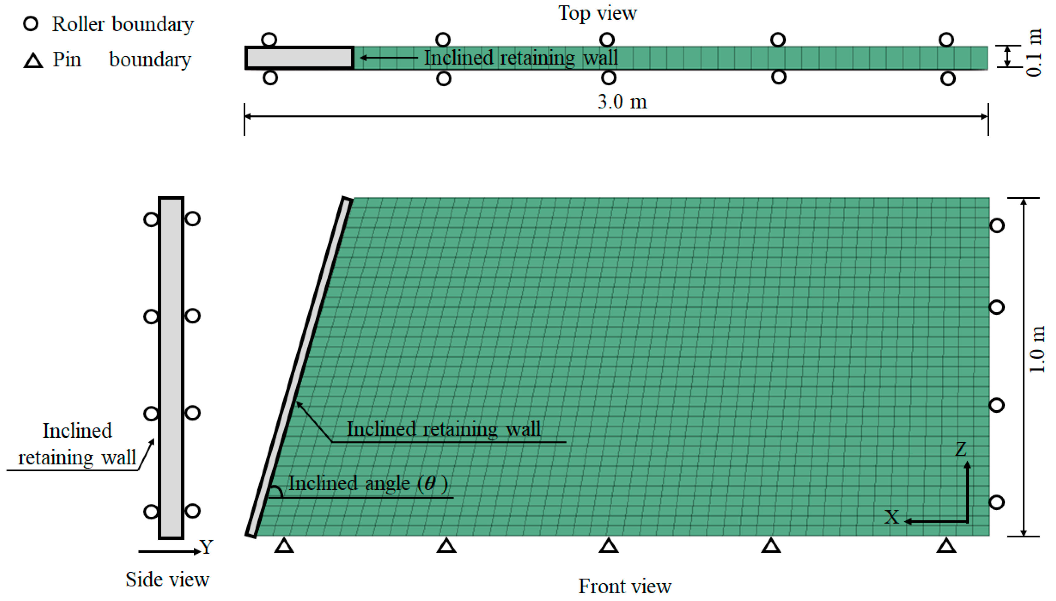
4.2. Comparison with Numerical Simulation Results of Inclined Retaining Walls

This study presents a comparison of numerical simulation results to address the lack of measured data for inclined retaining walls. All the finite-difference numerical model calculations in this paper are performed by FLAC 3D. Section 2 describes the model details, and Figure 1 presents the established model. Figure 8 shows the earth pressure comparison between the numerical simulation results and the proposed analytical results with various inclination angles. The inclination of the wall significantly affects the distribution of active earth pressure. As the inclination angle of the retaining walls changes from 0° to 10°, the normal active earth pressure at the same depth gradually decreases, which is consistent with Coulomb’s theory [2]. The earth pressure distribution gradually changes from a triangle to a curve with increasing inclination angle. Reasonable agreements between the measured, computed, and theoretical solutions are found. Cao’s [27] assumption of uniformly distributed vertical stress results in the calculated data of earth pressure being greater than the numerical data in the upper portion. The coincidence between the experimental and numerical simulations verifies the accuracy of the proposed analytical solution.

4.3. Comparison between Uniform and Nonuniform Distributions of Vertical Stress

Sand with an internal friction angle of 30° is used as the study object in this section. Figure 9 represents the distribution of the normal active stress acting on the wall (σ_w) with varying inclination and roughness of the retaining walls. When the inclination angle (θ) and the friction angle (δ) increase, the distribution of normal stress along the burial depth becomes more nonlinear, and the normal active stress decreases. An increased inclination angle and wall–soil interface roughness led to a higher maximum active stress position. Figure 9 compares the normal active stress under two vertical stress assumptions. At the same inclination angle, the calculation method considering the uniform distribution of vertical stress overestimates the vertical stress state, resulting in the shallow earth pressure being greater than that calculated from the proposed method. The earth pressure distribution, considering the nonuniform distribution of the vertical force, shows a more obvious soil arching effect under the same retaining wall roughness.

5. Conclusions

In this paper, the soil behind the retaining walls is divided into two zones based on its vertical stress distribution characteristics. A formula is established to describe the nonuniformly distributed vertical stress. An analytical solution is proposed for the active earth pressure of cohesionless soil acting on an inclined retaining wall. The proposed analytical solution describes the relationship between nonuniformly distributed vertical stresses of soil and earth pressure. The accuracy of the proposed analytical solution is demonstrated based on a comparison with experimental and numerical results. The following conclusions can be drawn:

(1)

As the inclination angle of the retaining wall increases, the normal active earth pressure on the inclined wall at the same depth gradually decreases.

(2)

The wall inclination has an obvious influence on the normal active earth pressure. The distribution of earth pressure gradually changes from a triangle to a curve with increasing inclination angle.

(3)

Compared with the traditional method, the proposed method considers the characteristics of a nonuniform distribution of vertical stress, resulting in a more accurate earth pressure calculation. The proposed method is helpful for the economic design of inclined retaining walls.

The earth pressure calculation method proposed in this paper is only applicable to sandy soil. Due to the complexity of clay, the proposed theory is not applicable to clay, and a calculation theory related to clay will be examined in future studies.

References

1. Zucca, M.; Valente, M. On the limitations of decoupled approach for the seismic behaviour evaluation of shallow multi-propped underground structures embedded in granular soils. Eng. Struct. 2020, 211, 110497. [Google Scholar] [CrossRef]
2. Rankine, W.J.M. II. On the stability of loose earth. Philos. Trans. R. Soc. 1857, 147, 9–27. [Google Scholar]
3. Coulomb, C.A. Essai sur une Application des Règles de Maximis et Minimis a Quelques Problèmes de Statique, Relatifs a l’Architecture; De l’Imprimerie Royale: Paris, France, 1776. (In French) [Google Scholar]
4. Lim, A.; Ou, C.Y.; Hsieh, P.G. Investigation of the integrated retaining system to limit deformations induced by deep excavation. Acta Geotech. 2018, 13, 973–995. [Google Scholar] [CrossRef]
5. Lim, A.; Ou Cyhsieh, P.G. A novel strut-free retaining wall system for deep excavation in soft clay: Numerical study. Acta Geotech. 2020, 15, 1557–1576. [Google Scholar] [CrossRef]
6. Wang, L.; Wu, C.; Tang, L.; Zhang, W.; Lacasse, S.; Liu, H.; Gao, L. Efficient reliability analysis of earth dam slope stability using extreme gradient boosting method. Acta Geotech. 2020, 15, 3135–3150. [Google Scholar] [CrossRef]
7. Paik, K.H.; Salgado, R. Estimation of active earth pressure against rigid retaining walls considering arching effects. Geotechnique 2003, 53, 643–645. [Google Scholar] [CrossRef]
8. Cai, Y.; Chen, Q.; Zhou, Y.; Nimbalkar, S.; Yu, J. Estimation of passive earth pressure against rigid retaining wall considering arching effect in cohesive-frictional backfill under translation mode. Int. J. Geomech. 2017, 17, 04016093. [Google Scholar] [CrossRef]
9. Li, J.; Wang, M. Simplified method for calculating active earth pressure on rigid retaining walls considering the arching effect under translational mode. Int. J. Geomech. 2014, 14, 282–290. [Google Scholar] [CrossRef]
10. Ni, P.; Song, L.; Mei, G.; Zhao, Y. On predicting displacement-dependent earth pressure for laterally loaded piles. Soils Found. 2018, 58, 85–96. [Google Scholar] [CrossRef]
11. Rao, P.; Chen, Q.; Zhou, Y.; Nimbalkar, S.; Chiaro, G. Determination of active earth pressure on rigid retaining wall considering arching effect in cohesive backfill soil. Int. J. Geomech. 2015, 16, 04015082. [Google Scholar] [CrossRef]
12. Goel, S.; Patra, N.R. Effect of arching on active earth pressure for rigid retaining walls considering translation mode. Int. J. Geomech. 2008, 8, 123–133. [Google Scholar] [CrossRef]
13. Patel, S.; Deb, K. Study of active earth pressure behind a vertical retaining wall subjected to rotation about the base. Int. J. Geomech. 2020, 20, 04020028. [Google Scholar] [CrossRef]
14. Khosravi, M.H.; Pipatpongsa, T.; Takemura, J. Experimental analysis of earth pressure against rigid retaining walls under transla-tion mode. Geotechnique 2013, 63, 1020–1028. [Google Scholar] [CrossRef]
15. Khosravi, M.H.; Pipatpongsa, T.; Takemura, J. Theoretical analysis of earth pressure against rigid retaining walls under translation mode. Soils Found. 2016, 56, 664–675. [Google Scholar] [CrossRef]
16. Lai, F.; Yang, D.; Liu, S.; Zhang, H.; Cheng, Y. Towards an improved analytical framework to estimate active earth pressure in nar-row c–ϕ soils behind rotating walls about the base. Comput. Geotech. 2022, 141, 104544. [Google Scholar] [CrossRef]
17. Zheng, G.; He, X.; Zhou, H.; Diao, Y.; Li, Z.; Liu, X. Performance and mechanism of batter-vertical framed retaining wall for ex-cavation in clay. Tunn. Undergr. Space Technol. 2022, 130, 104767. [Google Scholar] [CrossRef]
18. Zheng, G.; Liu, Z.; Zhou, H.; He, X.; Guo, Z. Behaviour of an outward inclined-vertical framed retaining wall of an excavation. Acta Geotech. 2022, 17, 5521–5532. [Google Scholar] [CrossRef]
19. Zheng, G.; Guo, Z.; Zhou, H.; Diao, Y.; Yu, D.; Wang, E.; He, X.; Tian, Y.; Liu, Z. Parametric studies of wall displacement in ex-cavations with inclined framed retaining walls. Int. J. Geomech. 2022, 22, 04022157. [Google Scholar] [CrossRef]
20. Zheng, G.; He, X.; Zhou, H. A Prediction Model for the Deformation of an Embedded Cantilever Retaining Wall in Sand. Int. J. Geomech. 2023, 23, 06023001. [Google Scholar] [CrossRef]
21. Handy, R.L. The arch in soil arching. J. Geotech. Eng. 1985, 111, 302–318. [Google Scholar] [CrossRef]
22. Segrestin, P. Design of Sloped Reinforced Fill Structures; Retaining Structures; Thomas Telford Publishing: London, UK, 1993; pp. 574–586. [Google Scholar]
23. Fang, Y.S.; Ishibashi, I. Static earth pressures with various wall movements. J. Geotech. Eng. 1986, 112, 317–333. [Google Scholar] [CrossRef]
24. Benmeddour, D.; Mellas, M.; Frank, R.; Mabrouki, A. Numerical study of passive and active earth pressures of sands. Comput. Geotech. 2012, 40, 34–44. [Google Scholar] [CrossRef]
25. Zhou, H.; Shi, Y.; Yu, X.; Xu, H.; Zheng, G.; Yang, S.; He, Y. Failure mechanism and bearing capacity of rigid footings placed on top of cohesive soil slopes in spatially random soil. Int. J. Geomech. 2023, 23, 04023110. [Google Scholar] [CrossRef]
26. Sitharam, T.G.; Maji, V.B.; Verma, A.K. Practical equivalent continuum model for simulation of jointed rock mass using FLAC3D. Int. J. Geomech. 2007, 7, 389–395. [Google Scholar] [CrossRef]
27. Cao, W.; Liu, T.; Xu, Z. Calculation of passive earth pressure using the simplified principal stress trajectory method on rigid retaining walls. Comput. Geotech. 2019, 109, 108–116. [Google Scholar] [CrossRef]
Figure 1. Numerical model.
Buildings 14 00076 g001
Figure 2. Comparison between the computed and experimental earth pressures [23].
Buildings 14 00076 g002
Figure 3. Vertical stress and principal stress distribution of soil behind walls: (a) a vertical wall, (b) an inclined wall with a 10° inclination angle, and (c) an inclined wall with a 20° inclination angle.
Buildings 14 00076 g003
Figure 4. Vertical stress field and distribution behind the inclined retaining wall: (a) vertical stress field distribution; (b) comparison result of numerical data and analytical solution.
Buildings 14 00076 g004
Figure 5. Trajectory of the major principal stress of soil.
Buildings 14 00076 g005
Figure 6. Forces acting on the horizontal element.
Buildings 14 00076 g006
Figure 7. Earth pressure comparison results from different theories [2,12,15,23].
Buildings 14 00076 g007
Figure 8. Earth pressure of different retaining walls [27].
Buildings 14 00076 g008
Figure 9. The distribution of active normal stress ( σ w ): (a) various inclination angles of the retaining wall, δ = 15° and (b) various wall–soil interface frictions, θ = 5°.
Buildings 14 00076 g009aBuildings 14 00076 g009b
Disclaimer/Publisher’s Note: The statements, opinions and data contained in all publications are solely those of the individual author(s) and contributor(s) and not of MDPI and/or the editor(s). MDPI and/or the editor(s) disclaim responsibility for any injury to people or property resulting from any ideas, methods, instructions or products referred to in the content.