
Elastic Local Buckling and Width-to-Thickness Limits of I-Beams Incorporating Flange–Web Interactions


Abstract
:1. Introduction
2. Finite Element Analysis
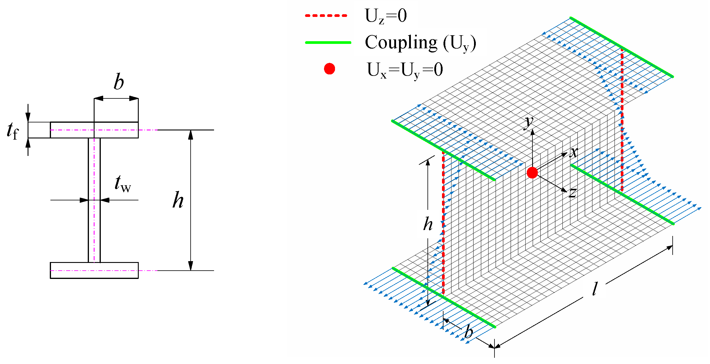
2.1. Finite Element Modeling
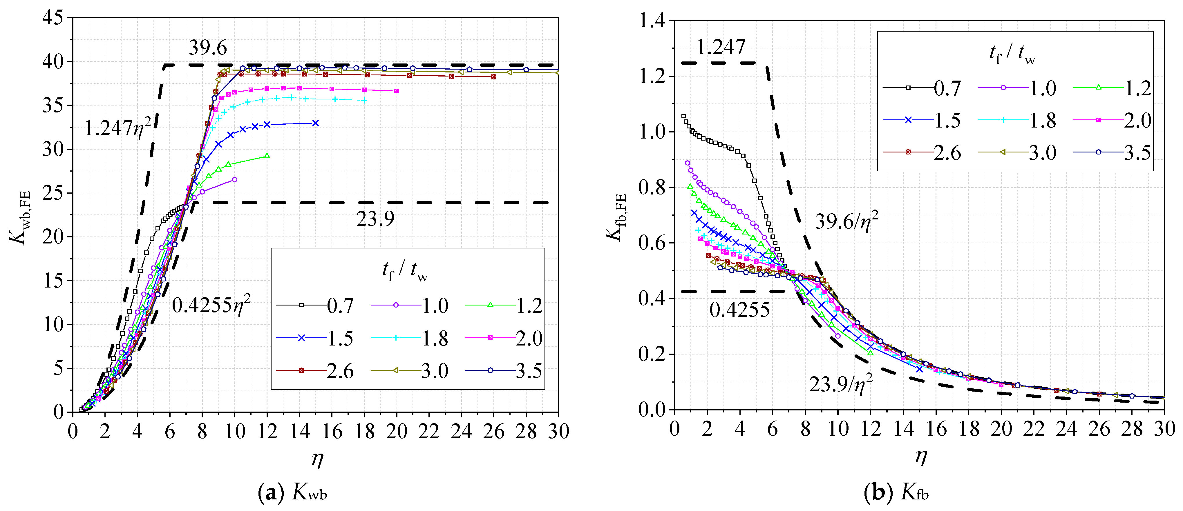
2.2. Results and Discussions
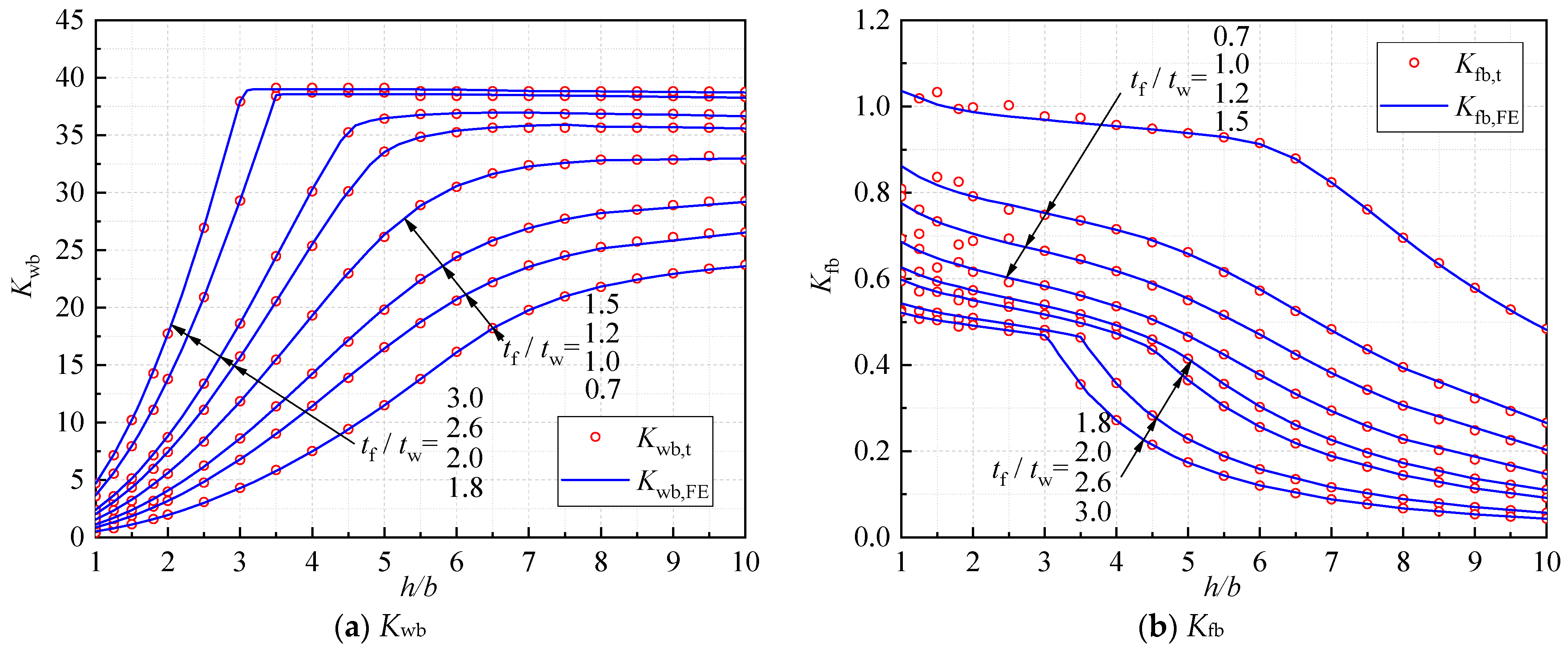
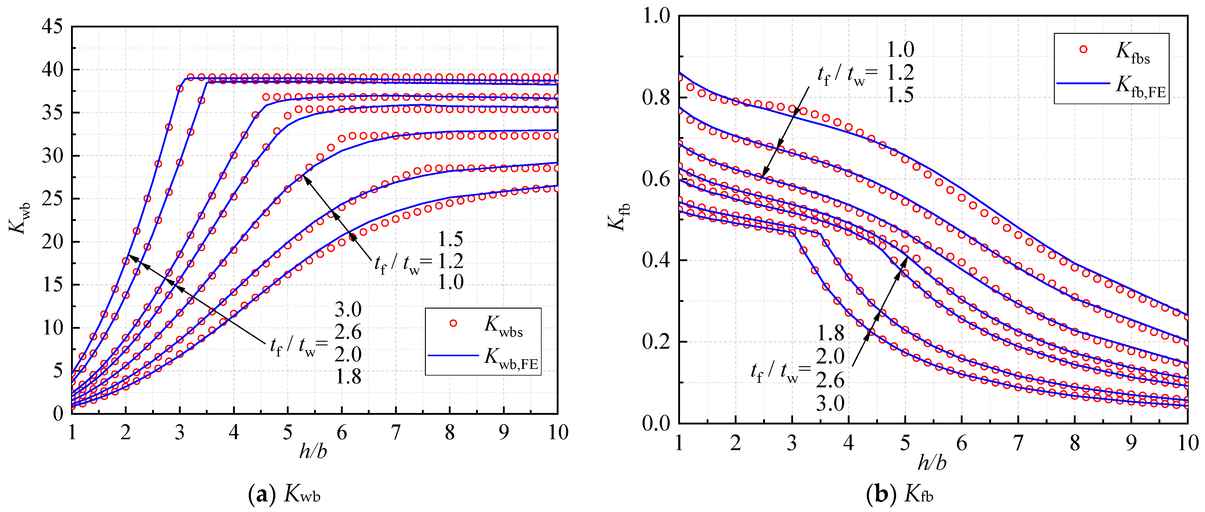
2.3. Comparison with Analytical Solutions
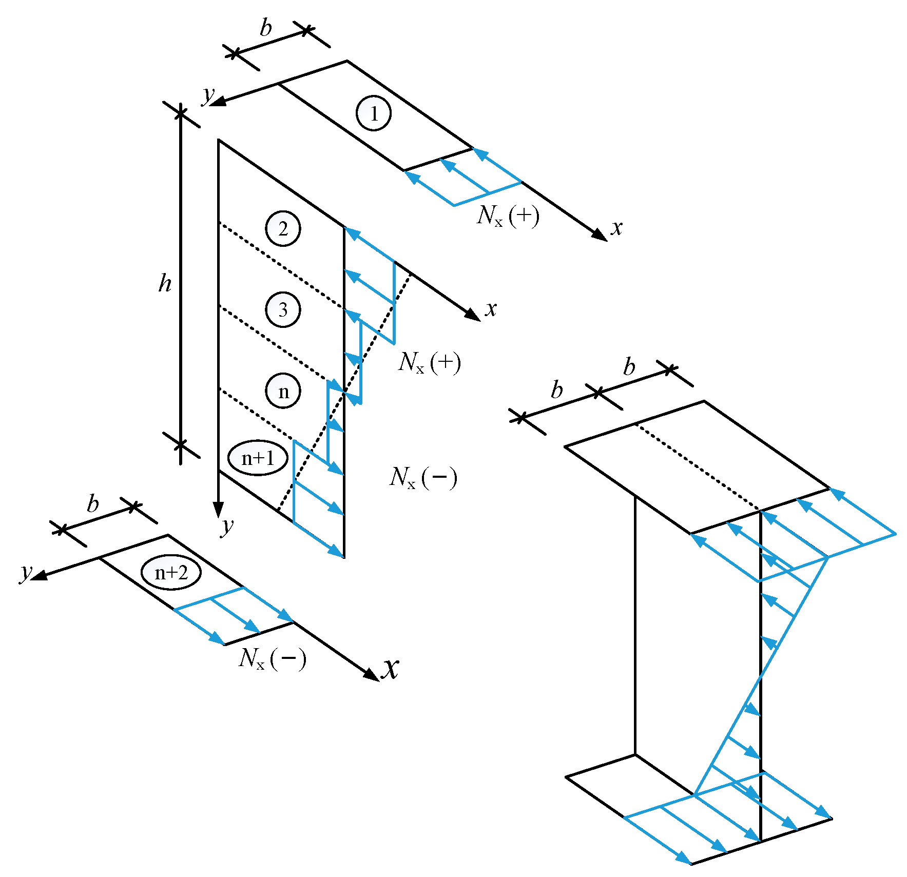
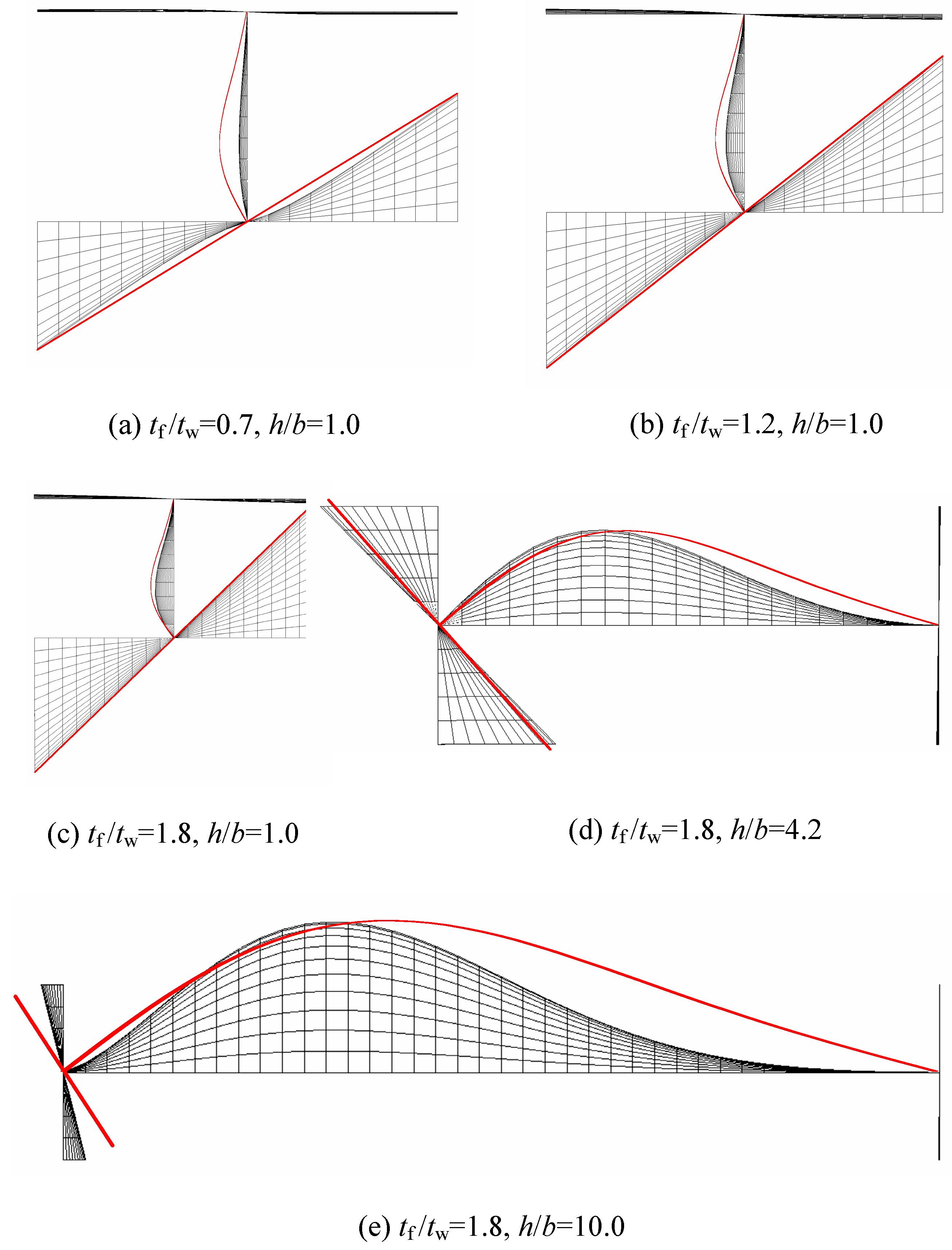
2.4. Buckling Mode
3. Simple Solution Development
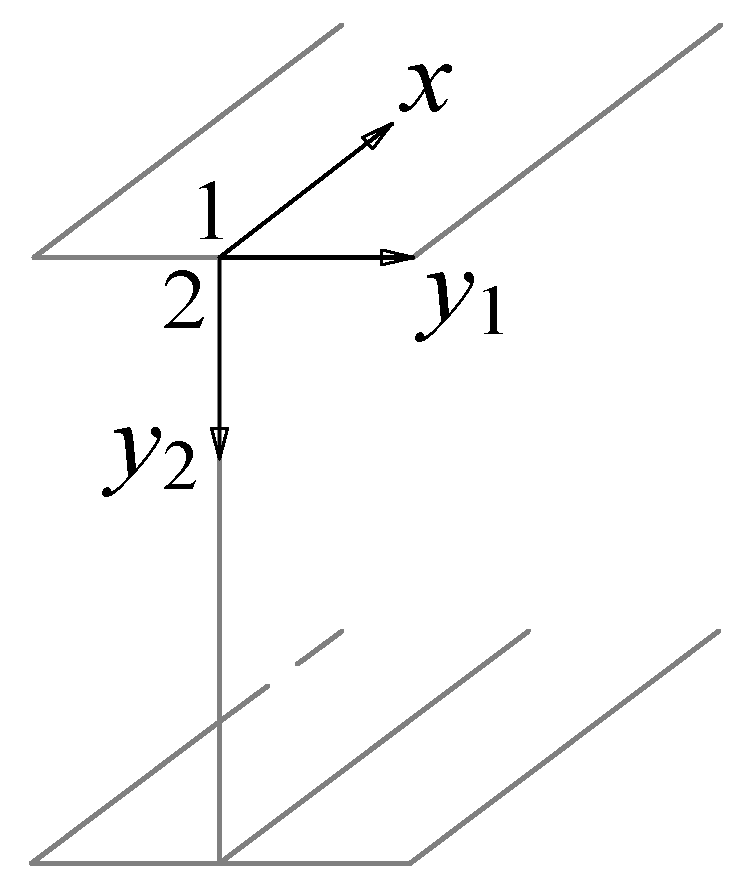
3.1. Energy Method
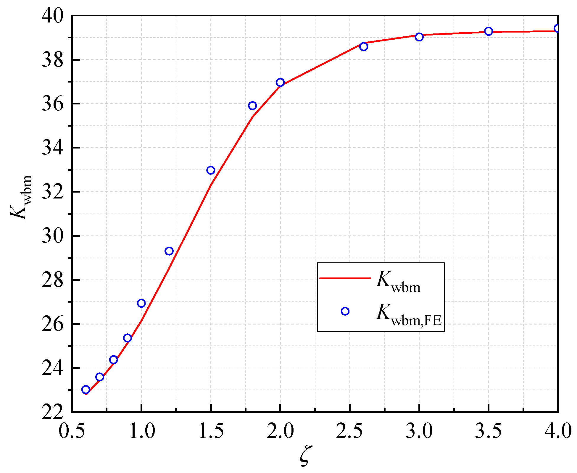
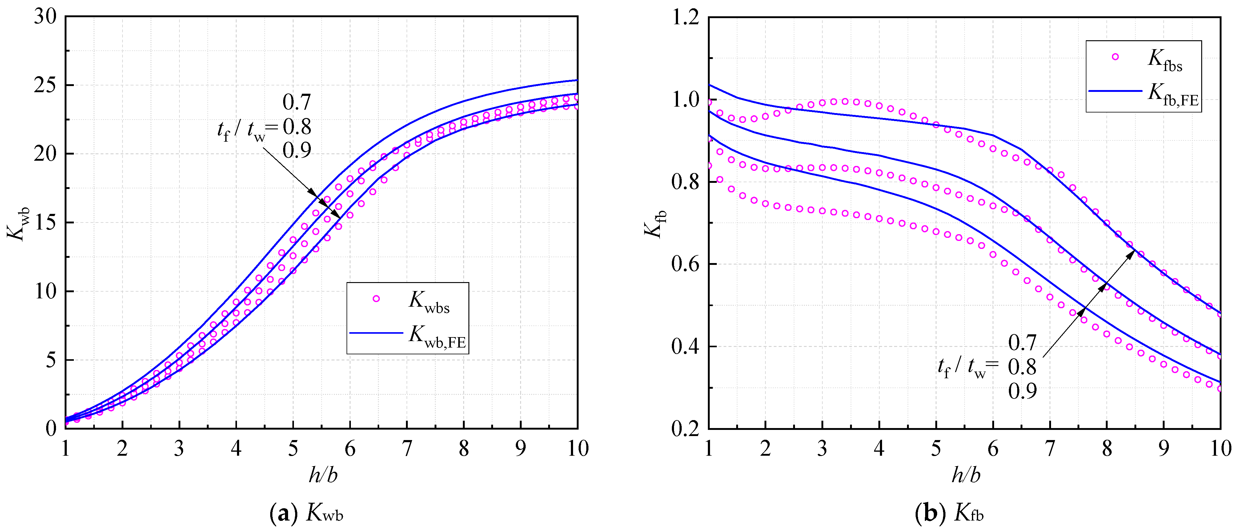
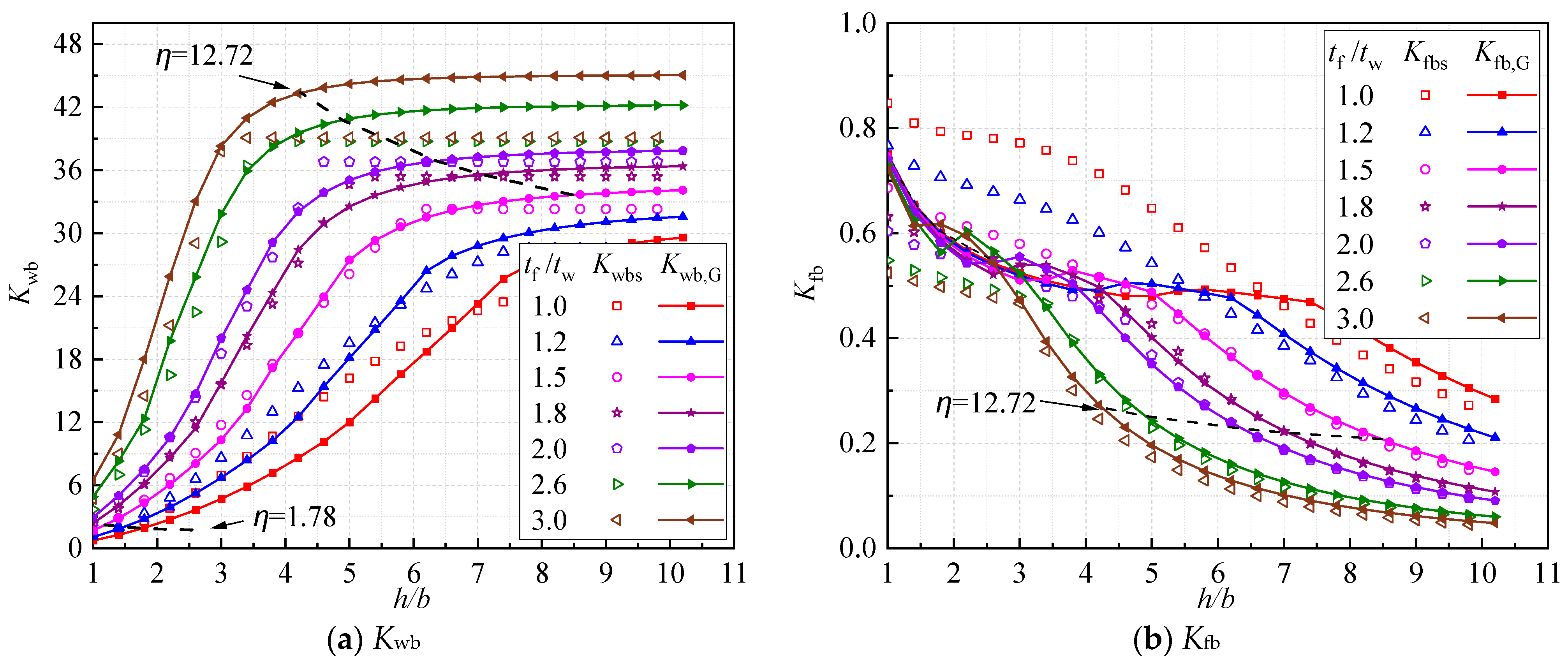
3.2. Comparison with Existing Solutions
4. Width-to-Thickness Limit for I-Section Beams
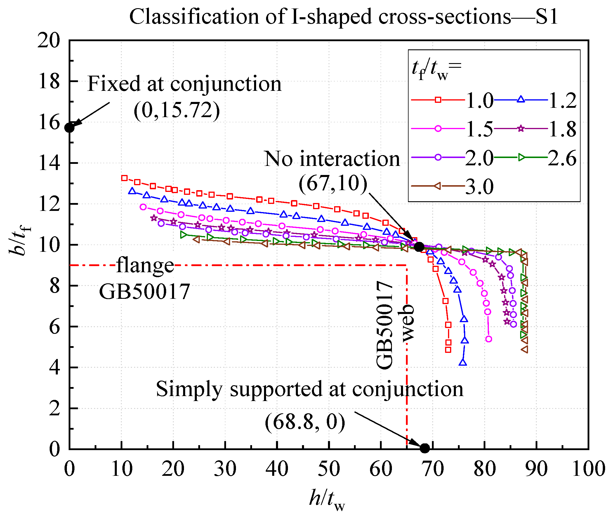
4.1. Method for the Determination of the Width-to-Thickness Limit
4.2. Revised Width-to-Thickness Limits
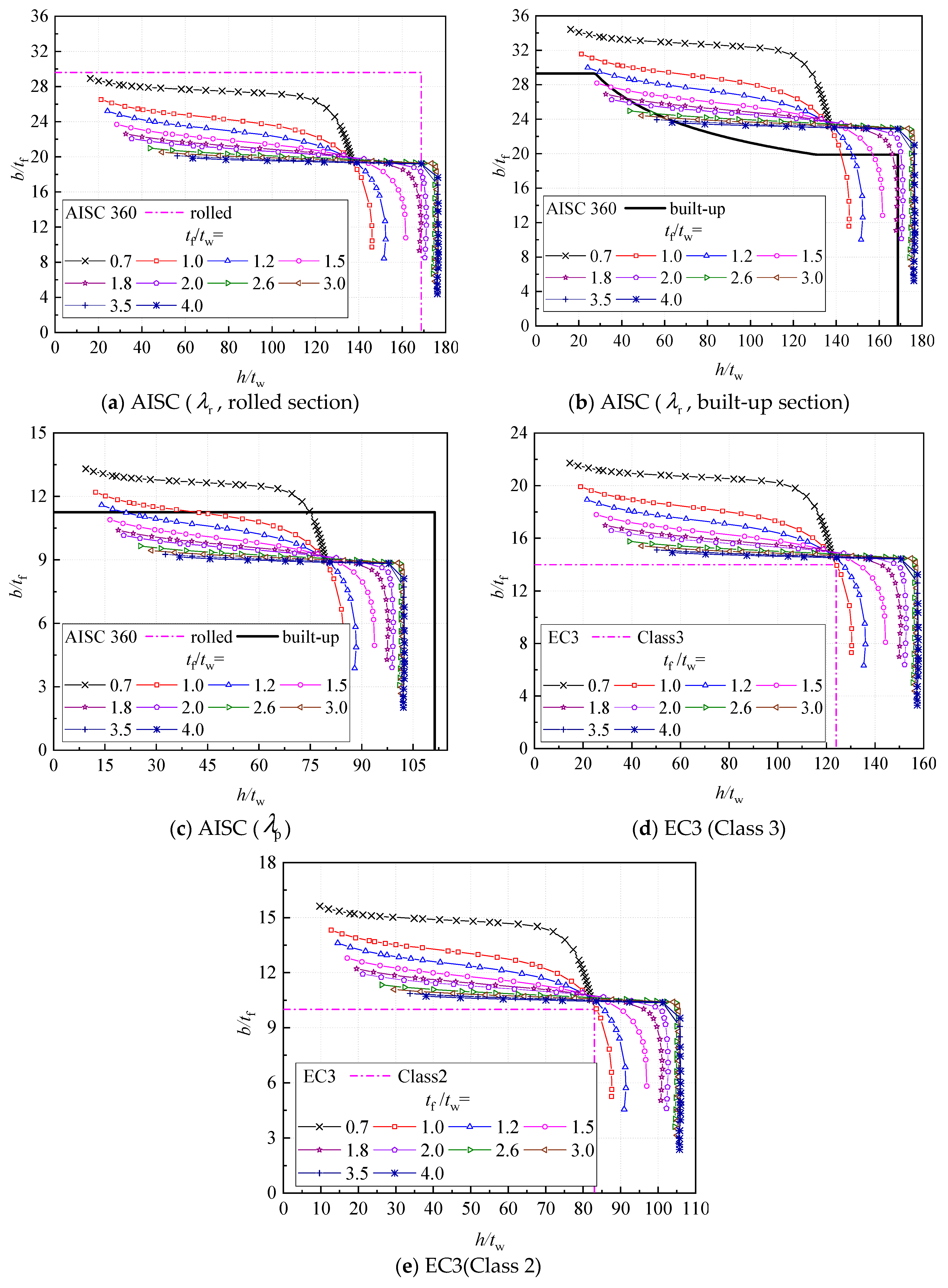
4.3. Evaluation of the Provisions of AISC and EC3
4.4. Comparison with Solutions in Existing Studies
5. Conclusions
Author Contributions
Funding
Data Availability Statement
Conflicts of Interest
References
- GB50017-2017; Standard for Design of Steel Structures. China Architecture & Building Press: Beijing, China, 2017.
- ANSI/AISC 360-16; Specification for Structural Steel Buildings. American Institute of Steel Construction: Chicago, IL, USA, 2016.
- EN 1993-1-1; Eurocode 3: Design of Steel Structures—Part 1-1: General Rules and Rules for Buildings. European Committee for Standardization: Brussels, Belgium, 2005.
- Bleich, F. Buckling Strength of Metal Structures; Mc Graw-Hill Book Company, Inc.: New York, NY, USA, 1952. [Google Scholar]
- Timoshenko, S.P.; Gere, J.M. Theory of Elastic Stability, 2nd ed.; McGraw-Hill: New York, NY, USA, 1961. [Google Scholar]
- Kroll, W.D.; Fisher, G.P.; Heimerl, G.J. Charts for Calculation of the Critical Stress for Local Instabilty of Columns with I-, Z-, Channel, and Rectangular-Tube Section; NACA: Washington, DC, USA, 1943. [Google Scholar]
- Lundquist, E.E.; Stowell, E.Z. Critical Compressive Stress for Flat Rectangualr Plates Supported along all Edges and Elastically Restrained against Rotation along the Unloaded Edges; NACA: Washington, DC, USA, 1942. [Google Scholar]
- Peng, G. The Research on Local Buckling of Thin-Walled Section. Master’s Thesis, Zhejiang University, Hangzhou, China, 2012. [Google Scholar]
- Seif, M.; Schafer, B.W. Local buckling of structural steel shapes. J. Constr. Steel Res. 2010, 66, 1232–1247. [Google Scholar] [CrossRef]
- Gardner, L.; Fieber, A.; Macorini, L. Formulae for Calculating Elastic Local Buckling Stresses of Full Structural Cross-sections. Structures 2019, 17, 2–20. [Google Scholar] [CrossRef]
- Jin, Y.; Tong, G. Elastic Buckling of Web Restrained by Flanges in I-section members. J. Zhejiang Univ. Eng. Sci. 2009, 43, 1883–1891. [Google Scholar]
- Vieira, L.; Gonçalves, R.; Camotim, D. On the local buckling of RHS members under axial force and biaxial bending. Thin Wall Struct. 2018, 129, 10–19. [Google Scholar] [CrossRef]
- Ragheb, W.F. Local buckling of welded steel I-beams considering flange–web interaction. Thin Wall Struct. 2015, 97, 241–249. [Google Scholar] [CrossRef]
- Johnson, D.L. An Investigation into the Interaction of Flanges and Webs in Wide-Flange Shapes. In Proceedings of the Annual Technical Session and Meeting, Cleveland, OH, USA, 16–17 April 1985; pp. 395–405. [Google Scholar]
- Zhang, Q.; Zhang, L.; Zhang, Y.; Liu, Y.; Zhou, J. Elastic Local Buckling of I-Sections under Axial Compression Incorporating Web–Flange Interaction. Buildings 2023, 13, 1912. [Google Scholar] [CrossRef]
- Wu, R.; Wang, L.; Tong, J.; Tong, G.; Gao, W. Elastic buckling formulas of multi-stiffened corrugated steel plate shear walls. Eng. Struct. 2024, 300, 117218. [Google Scholar] [CrossRef]
- Bulson, P.S. The Stability of Flat Plates; Chatto and Windus: London, UK, 1970. [Google Scholar]
- Szychowski, A. Computation of thin-walled cross-section resistance to local buckling with the use of the Critical Plate Method. Arch. Civ. Eng. 2016, 62, 229–264. [Google Scholar] [CrossRef]
- Szychowski, A.; Brzezińska, K. Local buckling and resistance of continuous steel beams with thin-walled I-shaped cross-sections. Appl. Sci. 2020, 10, 4461. [Google Scholar] [CrossRef]
- Chen, S.; Liu, J.; Chan, T. Local buckling behaviour of high strength steel and hybrid I-sections under axial compression: Numerical modelling and design. Thin Wall Struct. 2023, 191, 111079. [Google Scholar] [CrossRef]
- ANSYS. ANSYS Release 17.0 Documentation; ANSYS: Canonsburg, PA, USA, 2015. [Google Scholar]
- Ragheb, W.F. Local buckling analysis of pultruded FRP structural shapes subjected to eccentric compression. Thin Wall. Struct. 2010, 48, 709–717. [Google Scholar] [CrossRef]
- Tong, G. Out-of-Plane Stability of Steel Structures (Revised Version); China Architecture & Building Press: Beijing, China, 2012. [Google Scholar]
- EN 1993-1-5; Eurocode 3: Design of Steel Structures—Part 1-5: Plated Structrual Elements. European Committee for Standardization: Brussels, Belgium, 2006.
- Lukey, A.F.; Adams, P.F. Rotation capacity of beams under moment gradient. J. Struct. Div. 1969, 95, 1173–1188. [Google Scholar] [CrossRef]
- Yura, J.A.; Galambos, T.V.; Ravindra, M.K. The bending resistance of steel beams. J. Struct. Div. 1978, 104, 1355–1370. [Google Scholar] [CrossRef]


| Case | Flange-Dominated Mode | Weak Interaction | Web-Dominated Mode |
|---|---|---|---|
| tf/tw = 0.7 |  |  | |
| h/b = 1 | h/b = 10 | ||
| tf/tw = 1.2 | 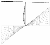 | 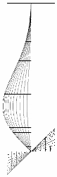 | 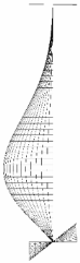 |
| h/b = 1 | h/b = 6.2 | h/b = 10 | |
| tf/tw = 1.8 | 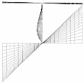 |  |  |
| h/b = 1 | h/b = 4.2 | h/b = 10 | |
| tf/tw = 2.6 |  |  |  |
| h/b = 1 | h/b = 2.8 | h/b = 10 | |
| Class | ||||
|---|---|---|---|---|
| S1 | S2 | S3 | S4 | |
| 67 | 81 | 94 | 107 | |
| 10 | 12 | 14 | 16 | |
Design Codes | Design Codes | In this Section | Design Codes | Design Codes | In this Section | |||
|---|---|---|---|---|---|---|---|---|
| AISC | Rolled I-shaped sections | Flange | 0.46 a | 0.46 | 1.0 a | 1.0 | ||
| Web | 0.58 a | 0.58 | 1.0 a | 1.0 | ||||
| Built-up I-shaped sections | Flange | 0.46 a | 0.46 | 1.19 a | 1.19 | |||
| Web | 0.58 a | 0.58 | 1.0 a | 1.0 | ||||
| EC3 | Flange | 0.54 b | 0.54 | 0.751 b 0.748 c | 0.751 | |||
| Web | 0.60 b | 0.60 | 0.893 b 0.874 c | 0.893 | ||||
Disclaimer/Publisher’s Note: The statements, opinions and data contained in all publications are solely those of the individual author(s) and contributor(s) and not of MDPI and/or the editor(s). MDPI and/or the editor(s) disclaim responsibility for any injury to people or property resulting from any ideas, methods, instructions or products referred to in the content. |
© 2024 by the authors. Licensee MDPI, Basel, Switzerland. This article is an open access article distributed under the terms and conditions of the Creative Commons Attribution (CC BY) license (https://creativecommons.org/licenses/by/4.0/).
Share and Cite
Zhang, L.; Zhang, Q.; Tong, G.; Zhu, Q. Elastic Local Buckling and Width-to-Thickness Limits of I-Beams Incorporating Flange–Web Interactions. Buildings 2024, 14, 347. https://doi.org/10.3390/buildings14020347
Zhang L, Zhang Q, Tong G, Zhu Q. Elastic Local Buckling and Width-to-Thickness Limits of I-Beams Incorporating Flange–Web Interactions. Buildings. 2024; 14(2):347. https://doi.org/10.3390/buildings14020347
Chicago/Turabian StyleZhang, Lei, Qianjing Zhang, Genshu Tong, and Qunhong Zhu. 2024. "Elastic Local Buckling and Width-to-Thickness Limits of I-Beams Incorporating Flange–Web Interactions" Buildings 14, no. 2: 347. https://doi.org/10.3390/buildings14020347