
Refined Analysis of Spatial Three-Curved Steel Box Girder Bridge and Temperature Stress Prediction Based on WOA-BPNN


Abstract
:1. Introduction
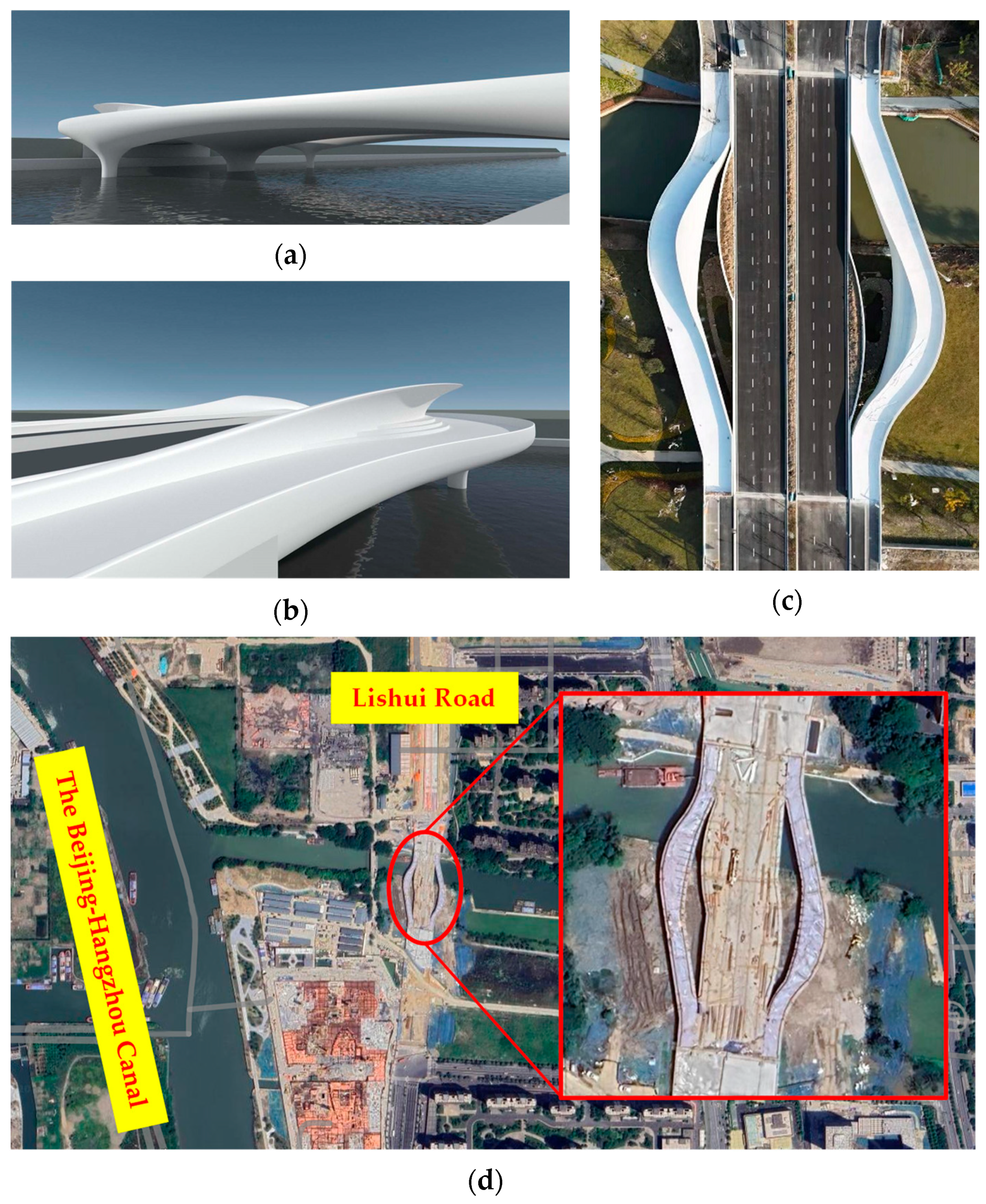
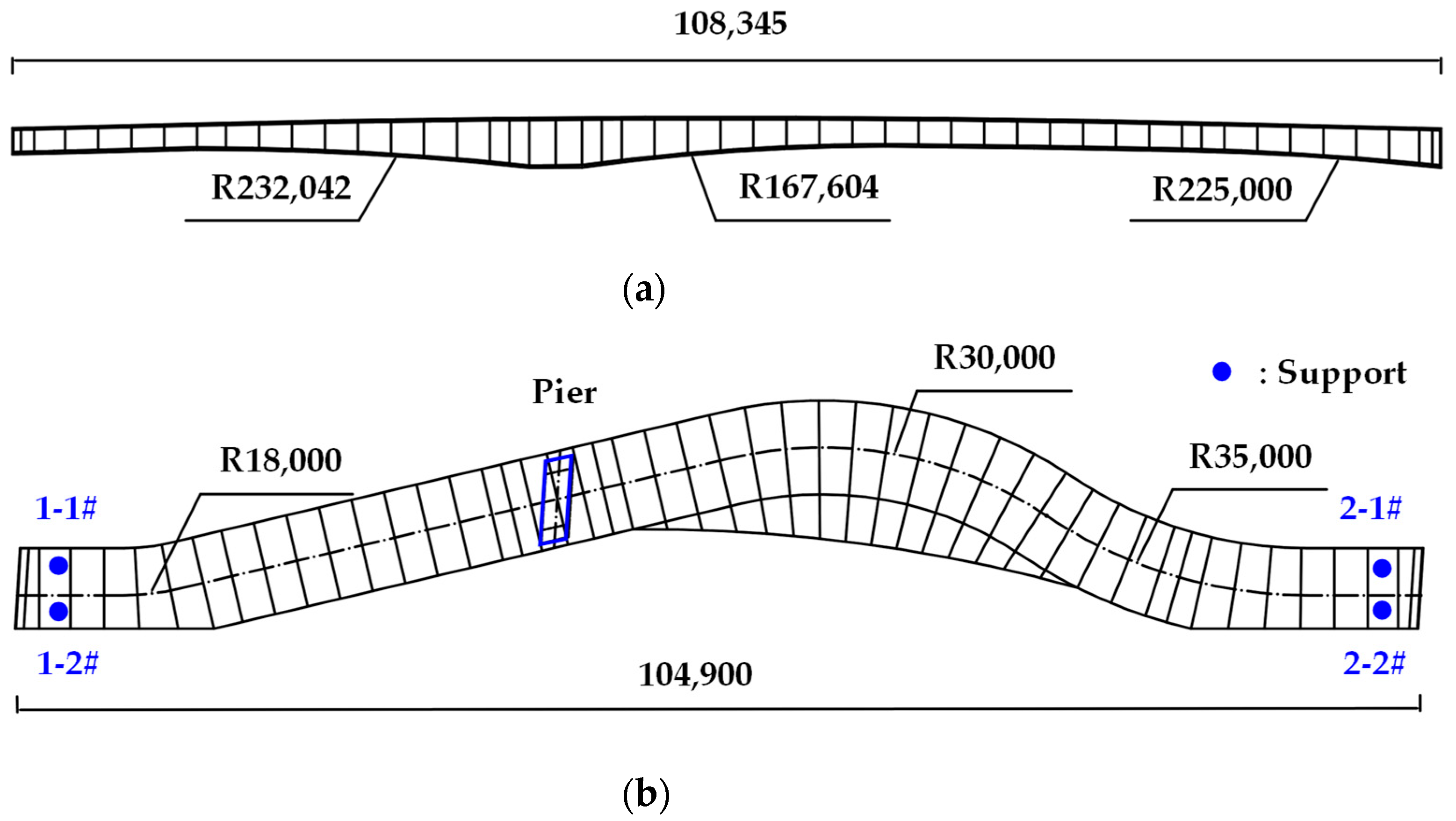
2. Bridge Description
3. Refined Finite Element Analysis
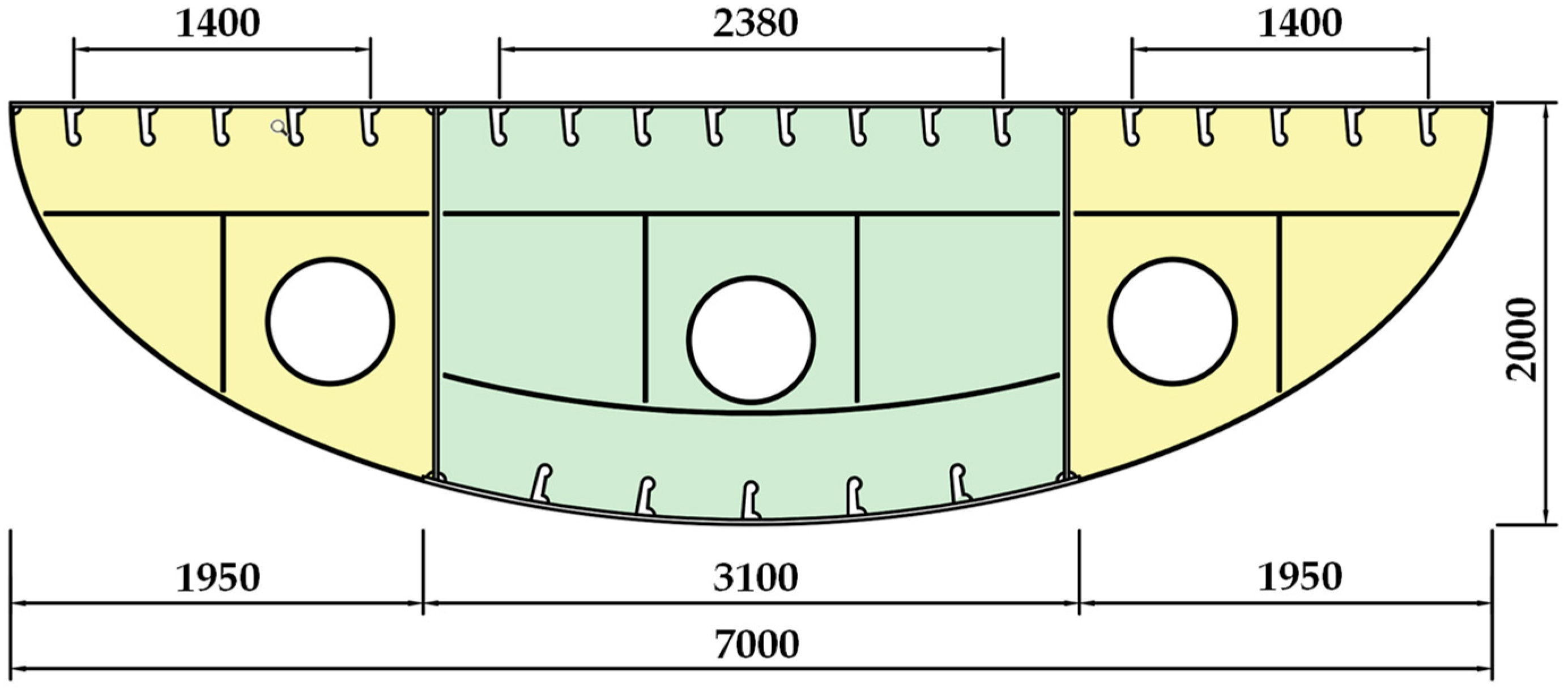
3.1. Modeling
3.2. Force Analysis
3.3. Stress Analysis
3.4. Curve Characterization
4. Temperature Gradient Effect Analysis
4.1. Temperature Gradient Distribution
4.2. Force Analysis
4.3. Stress Analysis
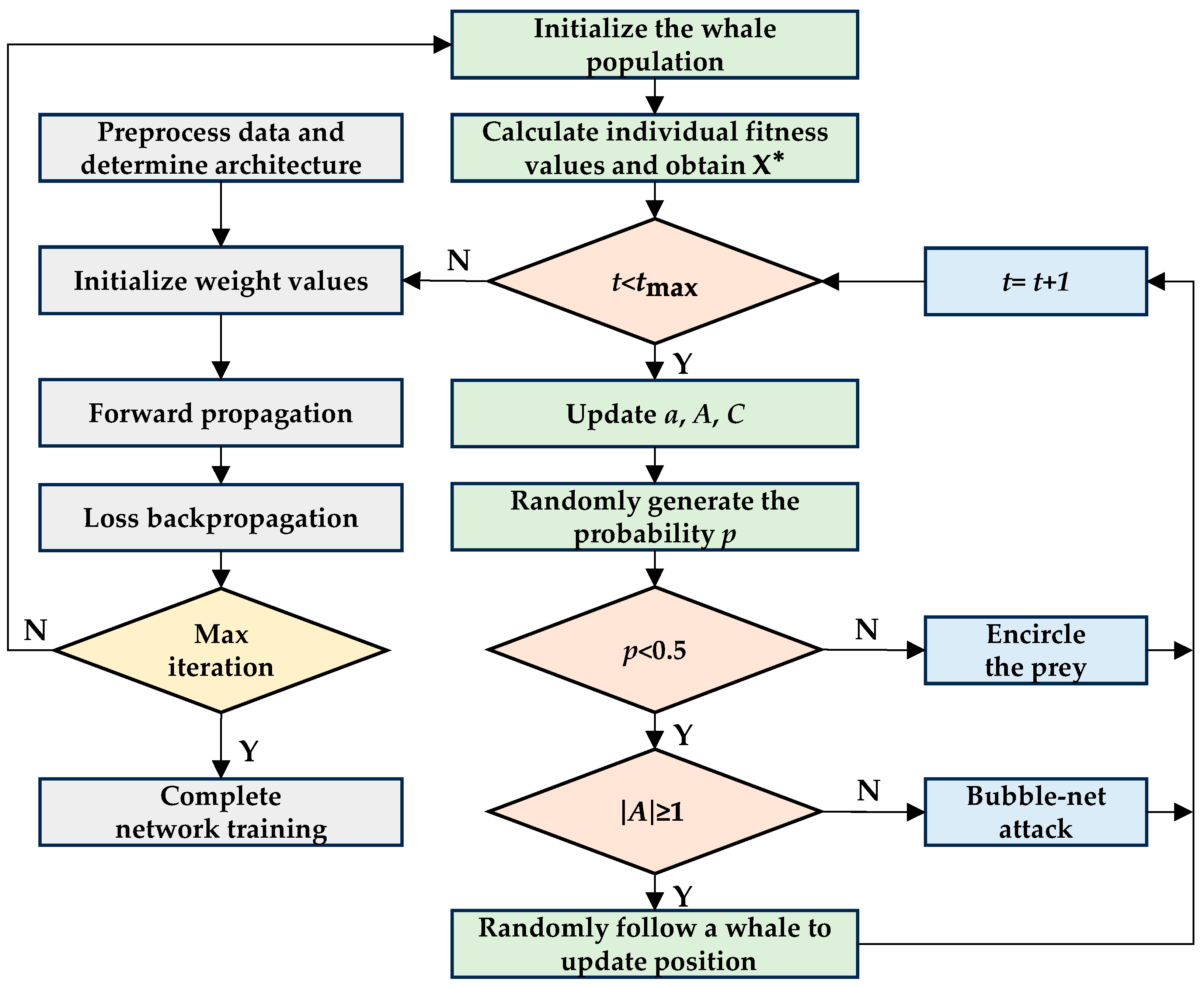
5. Neural Network Prediction
5.1. Methods
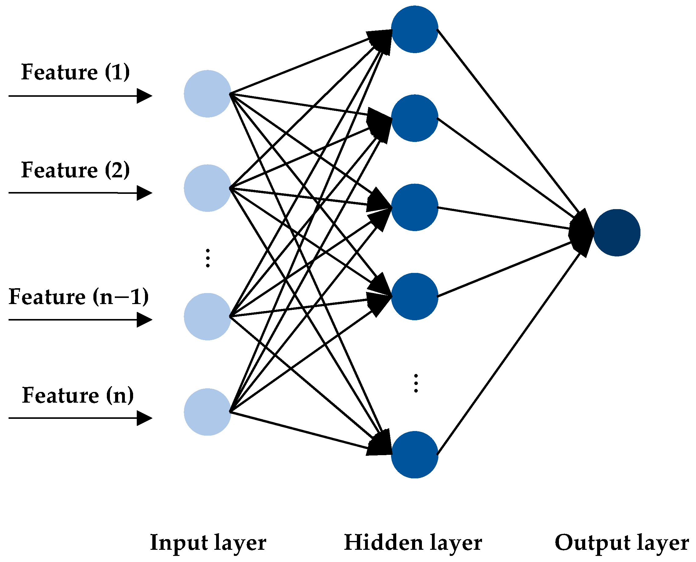
5.1.1. BPNN
5.1.2. WOA
5.1.3. WOA-BPNN
5.2. Evaluation Metric
5.3. Prediction Results
6. Conclusions
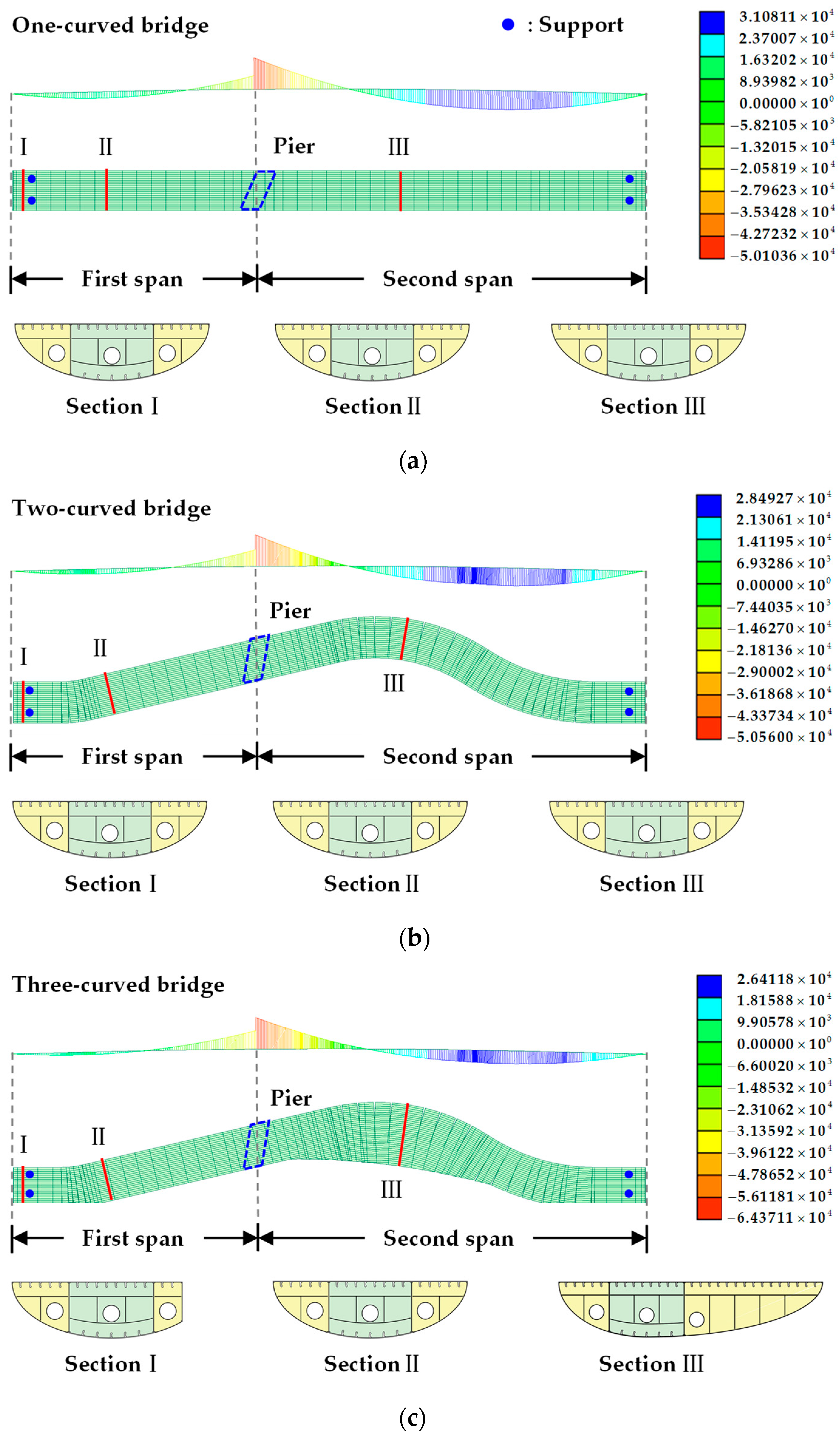
- A beam element model is established to analyze the general internal force of the bridge. The spatial three-curved steel box girder bridge exhibits spatial stress characteristics and a notable bending–torsion coupling effect. The bending and torsional moments at the cross-sections of the reverse curve section are relatively high.
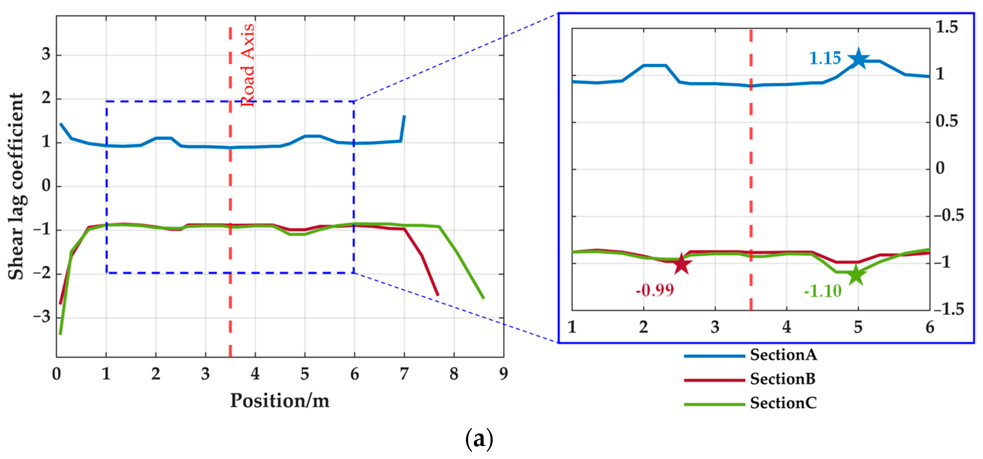
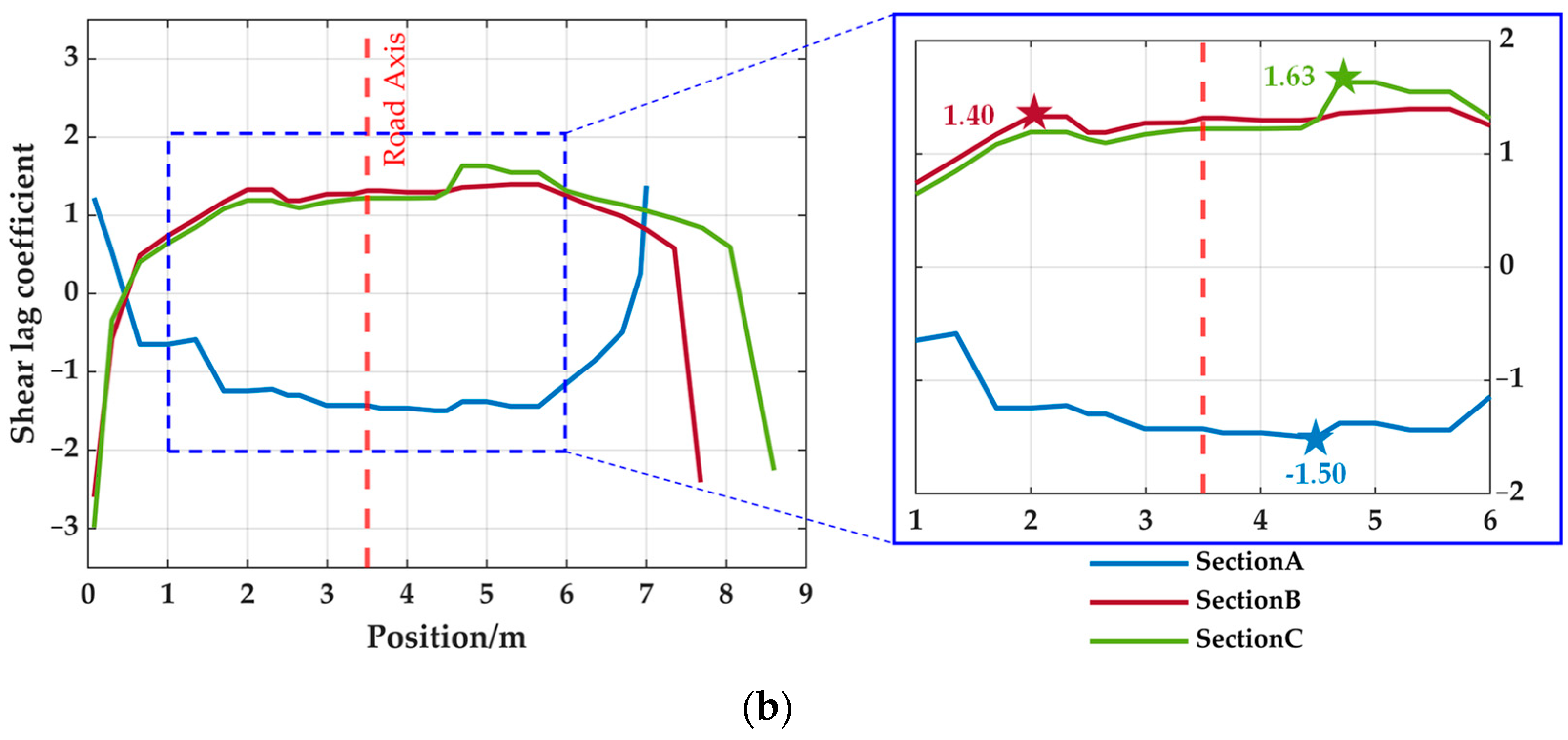
- A detailed stress analysis is performed on a plate element model. The shear lag effect is significant on the top and bottom plates of the steel box girder, and the widening of the cross-section aggravates the uneven stress distribution. In addition, severe stress concentration occurs at the vertices at both ends of the cross-section, with the maximum shear lag coefficient exceeding 3.
- Under the temperature effect, the three-curved steel box girder bridge displays a warped stress state. The torsion asymmetry phenomenon in the second span of the bridge intensifies the coupling effect of the bending and torsional moment.
- Under different temperature gradient modes, the temperature of the steel box girder’s bottom plate remains low and exhibits minimal changes. Compared to the BS-5400, the exponential temperature gradient pattern emphasizes a higher temperature gradient near the top plate of the cross-section, resulting in a 21% increase in average stress.
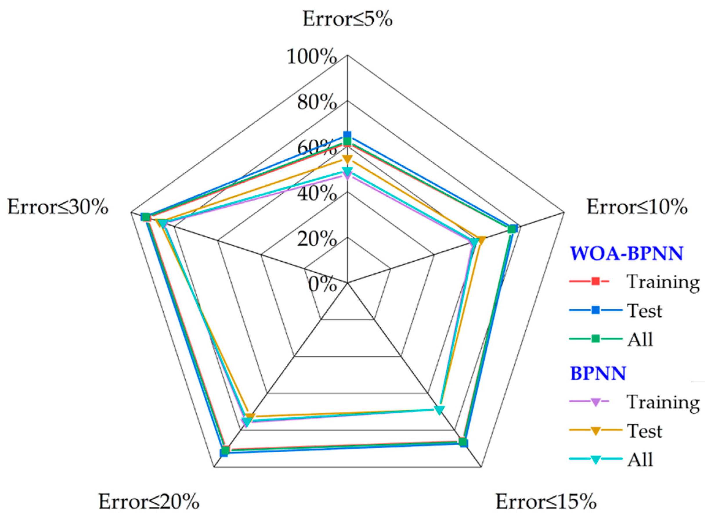
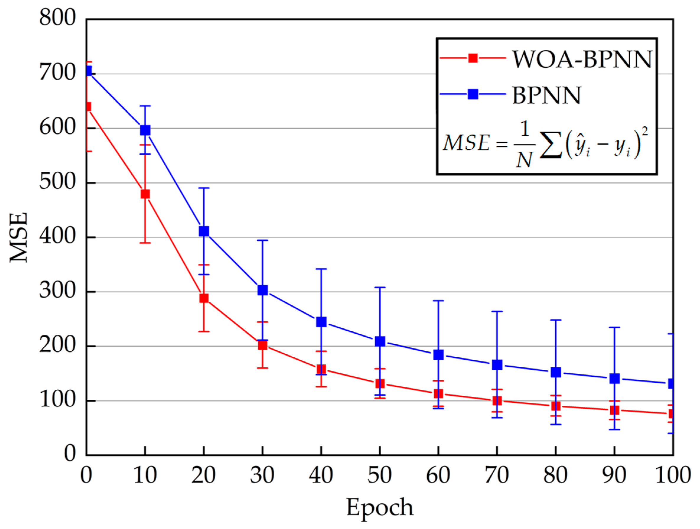
- Compared to BPNN, the use of the WOA algorithm to optimize the initial weight value can greatly improve the convergence speed of neural network training and the prediction accuracy of temperature gradient stress. The prediction accuracy of WOA-BPNN can reach over 90% with a 10% error tolerance and R2 of 0.99.
Author Contributions
Funding
Data Availability Statement
Conflicts of Interest
References
- Li, G.H.; Yu, Z.W.; Wang, Y.Z. Diseases of Curved Bridge and Temperature Effect. J. Highw. Trans. Res. Dev. 2008, 25, 58–63. [Google Scholar]
- Tong, Z.Y. Influence of Temperature Effect on Stress of Continuous Curved Box Girde. Railw. Eng. 2008, 11, 4–6. [Google Scholar]
- Zhang, J.D.; Zhang, Y.W.; Xing, S.L.; Zhu, J.P. Study of Temperature Effect of Concrete Curved Beam Bridge. World Bridge 2014, 42, 47–52. [Google Scholar]
- Liu, Y.J.; Liu, J.; Zhang, N. Review on Solar Thermal Actions of Bridge Structures. Civ. Eng. J. 2019, 52, 59–78. [Google Scholar]
- Liu, C. The Temperature Field and Thermal Effect of Steel-Concrete Composite Bridge. Ph.D. Thesis, Tsinghua University, Beijing, China, 2018. [Google Scholar]
- JTG D60-2015; General Specifications for Design of Highway Bridge and Culverts. China Communications Press: Beijing, China, 2015.
- BS 5400-2; Steel, Concrete and Composite Bridges (Part 2: Specification for Loads). Board of BSI: London, UK, 1978.
- Zhu, Z.W.; Wang, Y.J.; Li, J.P.; Teng, H.J. Comparison of Different Specification and Field Measurement on Vertical Temperature Gradient of Steel Box Girder. Stl. Constr. 2022, 37, 40–62. [Google Scholar]
- Teng, H.J.; Zhu, Z.W.; Li, J.P. Investigation on Vertical Temperature Gradient of Steel Box Girder with Steel Deck under Solar Radiation. J. Railw. Sci. Eng. 2021, 18, 3267–3277. [Google Scholar]
- Wang, Y.F.; Yang, H.Y.; Wang, Y.; Hao, J.; Xu, F.; Bai, C. Vertical Temperature Gradient Model of Steel Box Girder: Taking Steel Box Girder of Viaduct in Wuhan as Study Case. J. Wuhan Inst. Technol. 2021, 43, 202–220. [Google Scholar]
- Ding, Y.; Zhou, G.; Li, A.; Wang, G. Thermal Field Characteristic Analysis of Steel Box Girder Based on Long-Term Measurement Data. Int. J. Steel Struct. 2012, 12, 219–223. [Google Scholar] [CrossRef]
- Guo, F.; Zhang, S.; Duan, S. Analysis of Measured Temperature Field of Unpaved Steel Box Girder. Appl. Sci. 2022, 12, 8417. [Google Scholar] [CrossRef]
- Guo, F.; Zhang, S.; Duan, S.; Shen, Z.; Yu, Z.; Jiang, L.; He, C. Temperature Gradient Zoning of Steel Beams without Paving Layers in China. Case Stud. Constr. Mater. 2023, 18, e02054. [Google Scholar] [CrossRef]
- Editorial Department of China Journal of Highway and Transport. Review on China’s Bridge Engineering Research: 2021. J. Highw. Trans. 2021, 34, 1–97. [Google Scholar]
- Tian, G.; Xu, R.N.; Liao, C.Q.; Sun, C.Z. Temperature Estimation of Mass Concrete Structure Based on BP Neural Network. J. Water Resour. Archit. Eng. 2010, 8, 107–109, 123. [Google Scholar]
- Ying, M.; Zheng, Y.F.; Wang, D.J. Research of Arch Bridge Ring Temperature Field Based on BP Method. J. Harbin Inst. Technol. 2011, 43, 134–137. [Google Scholar]
- Wang, K.; Zhang, Y.; Liu, J.L.; He, X.H.; Cai, C.Z.; Huang, S.J. Prediction of Concrete Box-girder Maximum Temperature Gradientbased on BP Neural Network. J. Railway Sci. Eng. 2023, 1–11. [Google Scholar] [CrossRef]
- Wang, J.F.; Xu, Z.Y.; Fan, X.L.; Lin, J.P. Thermal Effects on Curved Steel Box Girder Bridges and Their Countermeasures. J. Perform. Constr. Facil. 2017, 31, 04016091. [Google Scholar] [CrossRef]
- Xu, Z.Y. The Temperature Fields of Curved Bridges with Steel Box Girder and their Effect. Master’s Thesis, Zhejiang University, Hangzhou, China, 2017. [Google Scholar]
- Yuan, J.; Lv, S.; Peng, X.; You, L.; Borges Cabrera, M. Investigation of Strength and Fatigue Life of Rubber Asphalt Mixture. Materials 2020, 13, 3325. [Google Scholar] [CrossRef] [PubMed]
- Mei, X.; Li, C.; Sheng, Q.; Cui, Z.; Zhou, J.; Dias, D. Development of a Hybrid Artificial Intelligence Model to Predict the Uniaxial Compressive Strength of a New Aseismic Layer Made of Rubber-Sand Concrete. Mech. Adv. Mater. Struct. 2023, 30, 2185–2202. [Google Scholar] [CrossRef]
- Liu, X.; Liu, Z.; Liang, Z.; Zhu, S.-P.; Correia, J.A.F.O.; De Jesus, A.M.P. PSO-BP Neural Network-Based Strain Prediction of Wind Turbine Blades. Materials 2019, 12, 1889. [Google Scholar] [CrossRef] [PubMed]
- Mirjalili, S.; Lewis, A. The Whale Optimization Algorithm. Adv. Eng. Softw. 2016, 95, 51–67. [Google Scholar] [CrossRef]


| Material | E (MPa) | γ (N/m3) | α (C−1) | µ |
|---|---|---|---|---|
| Q355 | 2.06 × 10⁵ | 7.85 × 10⁴ | 1.2 × 10⁻⁵ | 0.31 |
| C40 | 3.25 × 10⁴ | 2.5 × 10⁴ | 1 × 10⁻⁵ | 0.2 |
| Support | Force (kN) | RD (%) |
|---|---|---|
| 1-1# | 387.4 | 29.6 |
| 1-2# | 712.8 | |
| 2-1# | 973.4 | 19.8 |
| 2-2# | 1452.8 |
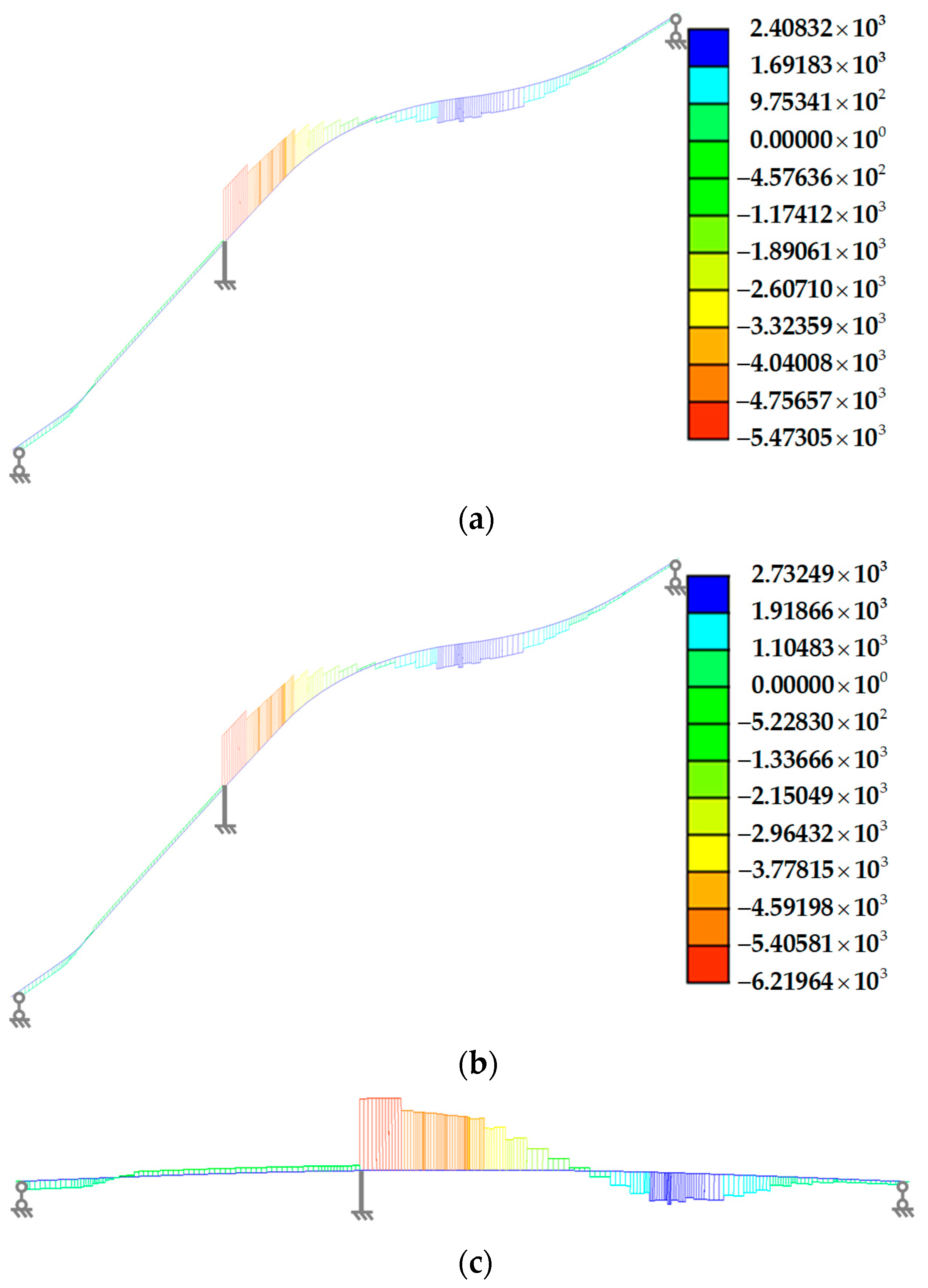
| Moment (kN·m) | BS-5400 | Wang et al. [18,19] |
|---|---|---|
| Mmax | 16,612.1 | 18,822.5 |
| Tmax | 2408.3 | 2732.5 |
| Tmin | 5473.1 | 6219.6 |
| Method | Support | Force (kN) | RD |
|---|---|---|---|
| BS-5400 | 1-1# | 28.6 | 86.0% |
| 1-2# | 379.5 | ||
| 2-1# | 232.3 | 75.2% | |
| 2-2# | 33 | ||
| Wang et al. [18,19] | 1-1# | 31.6 | 86.3% |
| 1-2# | 430.8 | ||
| 2-1# | 262.8 | 74.4% | |
| 2-2# | 38.6 |
| Section | BS-5400 | Wang et al. [18,19] | ||
|---|---|---|---|---|
| Tensile Stress (MPa) | Compressive Stress (MPa) | Tensile Stress (MPa) | Compressive Stress (MPa) | |
| A | 26.5 | 39.2 | 27.8 | 48.0 |
| B | 15.3 | 26.6 | 17.0 | 33.0 |
| C | 19.0 | 27.2 | 26.8 | 33.5 |
| Dataset | a10 | a20 | R2 | MAE (MPa) | MAPE | |
|---|---|---|---|---|---|---|
| BPNN | Training | 75.75% | 84.60% | 0.97 | 3.33 | 4.27 |
| Test | 72.60% | 86.60% | 0.97 | 3.28 | 4.44 | |
| All | 75.00% | 85.24% | 0.97 | 3.30 | 4.29 | |
| WOA-BPNN | Training | 90.55% | 92.45% | 0.99 | 2.13 | 4.87 |
| Test | 92.36% | 93.64% | 0.99 | 2.02 | 5.78 | |
| All | 91.05% | 92.98% | 0.99 | 2.08 | 4.94 | |
Disclaimer/Publisher’s Note: The statements, opinions and data contained in all publications are solely those of the individual author(s) and contributor(s) and not of MDPI and/or the editor(s). MDPI and/or the editor(s) disclaim responsibility for any injury to people or property resulting from any ideas, methods, instructions or products referred to in the content. |
© 2024 by the authors. Licensee MDPI, Basel, Switzerland. This article is an open access article distributed under the terms and conditions of the Creative Commons Attribution (CC BY) license (https://creativecommons.org/licenses/by/4.0/).
Share and Cite
Hu, W.; Zhang, Z.; Shi, J.; Chen, Y.; Li, Y.; Feng, Q. Refined Analysis of Spatial Three-Curved Steel Box Girder Bridge and Temperature Stress Prediction Based on WOA-BPNN. Buildings 2024, 14, 415. https://doi.org/10.3390/buildings14020415
Hu W, Zhang Z, Shi J, Chen Y, Li Y, Feng Q. Refined Analysis of Spatial Three-Curved Steel Box Girder Bridge and Temperature Stress Prediction Based on WOA-BPNN. Buildings. 2024; 14(2):415. https://doi.org/10.3390/buildings14020415
Chicago/Turabian StyleHu, Wei, Zhongyong Zhang, Junwei Shi, Yulun Chen, Yixuan Li, and Qian Feng. 2024. "Refined Analysis of Spatial Three-Curved Steel Box Girder Bridge and Temperature Stress Prediction Based on WOA-BPNN" Buildings 14, no. 2: 415. https://doi.org/10.3390/buildings14020415
APA StyleHu, W., Zhang, Z., Shi, J., Chen, Y., Li, Y., & Feng, Q. (2024). Refined Analysis of Spatial Three-Curved Steel Box Girder Bridge and Temperature Stress Prediction Based on WOA-BPNN. Buildings, 14(2), 415. https://doi.org/10.3390/buildings14020415