Abstract
Equivalent viscous damping plays a central role in displacement-based design procedures. In this paper, approaches for estimating the equivalent viscous damping of RC frame buildings are proposed. At first, the analytical formulation of Blandon and Priestley was analysed, and then a calibration of the coefficients of this formulation was performed. Compared with the work of Blandon and Priestley, a larger set of synthetic accelerograms, related to different types of soil and different intensities, and a wider range of the effective periods were considered. In particular, two different sets of parameters are proposed: the first is usable in the case of spectra obtained numerically (approach 1), and the second is usable in the case of code-based spectra and damping modification factor (approach 2). To test the performed calibration and to compare the considered formulations (i.e., the proposed and literature equations), the direct displacement-based design procedure has been applied to three case studies of reinforced concrete frame structures, and then pushover and nonlinear time-history analyses have been performed. The results show that the use of the calibrated parameters (for both the considered approaches) has determined more conservative results, in terms of design base shear and maximum drift from NLTH. Moreover, the average displacement profiles and the inter-storey drifts obtained from time-history analyses for the frames designed with the calibrated parameters match better the design profile.
1. Introduction
Nowadays, design codes include force-based design methods to define the capacity and the demand of structural systems under seismic actions. However, critical aspects characterize the traditional force-based approaches, and displacement-based design approaches have been proposed to overcome such issues [1,2,3,4,5]. Among the different approaches proposed in the literature [6,7], a widespread method is direct displacement-based design (DDBD) [1]: in this approach, structures are designed with a direct procedure to achieve displacements related to specific limit states. Specifically, the basic idea behind the approach is to identify the optimal structural strength to obtain a selected performance limit state, which is related to a given level of damage, for a specified level of seismic intensity [8].
The DDBD relies on the concept of equivalent structure developed in the pioneering work by Shibata and Sozen [9], which characterizes the structure by means of two parameters, i.e., the secant stiffness related to maximum displacement [10] and the equivalent viscous damping (EVD), which represent the effects of both elastic and hysteretic damping. Errors in the estimation of the latter parameter can lead to consequent errors in the design procedure [11]. Specifically, hysteretic damping is used to model the dissipating behaviour of the structure and is related to the hysteretic energy dissipated during the inelastic response [8]. In the DDBD procedure, the equivalent viscous damping is used to select the appropriate damped displacement spectrum.
The DDBD approach belongs to the methods for so-called “deformation-specification based design”, and the transition to these methods from the traditional force-based approaches has been characterized by different steps [8]. The first stage was characterized by the approaches known as “force-based/displacement checked”, i.e., an improvement to the force-based design approaches, where emphasis is placed on the calculation of the displacement demand for structures designed using force-based approaches. An advancement of this approach consisted of the so-called “deformation-calculation based design”, where attention is paid to the detailing of critical sections (e.g., transverse reinforcement of RC elements) as a function of the local deformation demand. Finally, in the “deformation-specification based design” approach the structure is designed to reach a specified deformation state when subjected to the design-level earthquake [8].
Kumbhar et al. [12] analysed the efficiency of various DDBD approaches for RC buildings by considering the most important parameters that characterizes the different approaches, such as target displacement profile, equivalent viscous damping, and base shear distribution pattern. In [13] a simplified displacement-based assessment was applied for direct monetary loss estimation of a RC frame building damaged during the 2009 L’Aquila earthquake. In [14] a simplified pushover analysis approach for RC frame structures was proposed. In general, the results of pushover analyses are useful to define the behaviour of equivalent single-degree-of-freedom structures, thus enabling the possibility of using simplified seismic assessment procedures such as the displacement-based assessment [8].
Equivalent viscous damping was usually estimated by using the methodology proposed by Jacobsen [15], which, however, assumes complete loops in the hysteretic models under sinusoidal excitation. Subsequent studies, such as those proposed by Miranda and Garcia [16] and by Priestley and Grant [17], have shown how Jacobsen’s approach tends to overestimate this parameter for some hysteretic models. Blandon and Priestley [18] proposed a new methodology for the evaluation of equivalent viscous damping, based on an iterative procedure using nonlinear time-history analyses of single degree of freedom structures. The equations proposed by Blandon and Priestley have been obtained by using six synthetic accelerograms, compatible with the ATC32 design spectrum for soil type C and PGA 0.7 g [18], and by considering a range of effective periods equal to 0.5–4 s.
Research on the estimation of the equivalent viscous damping in the context of DDBD approaches has continued in research years by focusing on a variety of different structures; for example: steel members [19], infilled RC frames [20], linked-column steel frame structures [21], RC frame structures with BRBs [22], and steel moment-resisting framed structures with dissipative beam-to-column partial-strength joints [23]. In the work of Gu and Shen [24], the influence of different formulations of the EVD on the DDBD procedure has been assessed by considering un-bonded post-tensioned concrete wall systems. In [25] the displacement-based assessment procedure is extended to infilled RC frames, by studying two fundamental steps of the process, i.e.,: the estimation of the EVD and the identification of the limit-state displacement profile. DDBD approaches have been also applied to timber structures, as shown in [26,27], which focus, respectively, on cross laminated timber building structures and glue-laminated timber frame with BRBs. The estimation of the EVD in the context of DDBD was also performed for non-structural building elements and special structures: in [28] a calibrated EVD was proposed for suspended piping trapeze restraint installations, while in [29] the formulation of the EVD was proposed for pallet-type steel storage racks.
In this paper, the results obtained with the formulation of Blandon and Priestley [18] for the evaluation of equivalent viscous damping have been analysed, and two modified sets of coefficients, obtained through an extensive calibration procedure, are proposed. Compared with the work of Blandon and Priestley [18], this has been carried out by considering a larger set of synthetic accelerograms, related to different types of soil and different intensities, and by considering a wider range of the effective periods. By operating in this way, the original expression proposed by Blandon and Priestley [18] has been maintained unchanged; only the coefficients of the expression have been varied. The main objective of this study is a comparison between the application of the equations with the proposed calibrated coefficients and the equations proposed in the literature.
Firstly, in order to calibrate the equivalent damping equations, the analytical computation of displacement-damped spectra from site accelerometric records has been used. Then, the calibration procedure has been repeated with the Eurocode 8 [30] design spectrum and the Damping Reduction Factor (DRF) η for the evaluation of reduced damped displacement spectra. In this way, it has been possible to obtain two different sets of parameters to be used in equivalent viscous damping equations according to the methodology chosen to obtain the displacement damped spectra.
Furthermore, a comparison between the response predicted in the design of a set of reinforced concrete (RC) structures by using the DDBD procedure with the calibrated damping equations and those from the literature, and the response obtained from nonlinear time-history analyses has been performed.
2. Materials and Methods
2.1. Modelling Equivalent Viscous Damping
According to the DDBD procedure, the real structure with multiple degrees of freedom (MDOF) is associated with an equivalent single-degree-of-freedom system (SDOF), characterized by a secant stiffness and an equivalent viscous damping index, which takes into account the nonlinear behaviour of the structure.
The equation proposed by Priestley et al. [8] to compute the equivalent viscous damping is composed of two parts:
where represents the initial damping in the elastic phase, and represents the energy dissipation due to nonlinear hysteretic behaviour.
The initial elastic damping, usually set at 5%, should represent the energy dissipation when the structure is in the elastic range. However, it is not clear whether the use of this constant coefficient is suitable for the inelastic response of structures, since hysteretic models usually include the entire energy dissipation [18]. Therefore, both in the latter study and in the present research, the influence of elastic damping has been removed from the DDBD process and the time-history analysis, in order to investigate only the hysteretic component.
There are several references [3,31,32,33,34] which propose different equivalent viscous damping formulations, some based on the Jacobsen method, others on time-history analyses results. Some of the main equations are listed in Table 1.

Table 1.
Literature equivalent viscous damping equations.
In general, the formulation proposed by Priestley [3], for different hysteretic laws, has the following aspect:
where indicates the initial viscous damping, μ is the ductility level, and and are parameters depending on the hysteretic model and on the type of structure. It can be noticed that equivalent damping index varies according to the structural system and in some cases even within the same type of structure; this can lead to different evaluations of the target displacement in a DDBD procedure.
Previous studies in the literature indicate that the use of Jacobsen’s approach for equivalent viscous damping is characterized by some problems. Dwairi and Kowalsky [35] pointed out that, in the case of sinusoidal excitation, Jacobsen’s approach tends to overestimate the displacements for period less than the sine wave fundamental period: when using natural accelerograms, this approach tends to overestimate the equivalent viscous damping in case of hysteretic models characterized by large loops, involving an underestimation of displacements. Blandon and Priestley [18] confirmed that Jacobsen’s approach tends to overestimate the equivalent viscous damping especially for hysteretic models with high energy dissipation capacity. In their study, Blandon and Priestley [18] have identified a methodology which is able to provide more precise and reliable equivalent viscous damping equations. The results proposed in the aforementioned study led to the following formulation, assuming :
which can be also expressed as:
where a, b, c, d are coefficients defined according to the considered hysteretic model, μ indicates the ductility level, the effective period (according to secant stiffness), and N is the normalization factor:
The innovative aspect compared to previous formulations consists of the term depending on the effective period.
2.2. Procedure for the Calibration of Equivalent Viscous Damping Equations
The equations proposed by Blandon and Priestley [18] have been obtained by using the data from nonlinear time-history analyses of single-degree-of-freedom systems, characterized by different effective periods and ductility levels, subjected to 6 synthetic accelerograms. In this paper, a large set of analyses has been performed in order to propose modified coefficients for the relation (4) using the same algorithm proposed by Blandon and Priestley [18] (Figure 1).
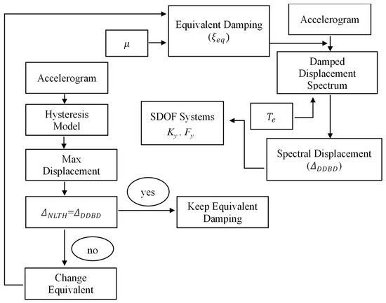
Figure 1.
Verification algorithm proposed by Blandon and Priestley [18].
2.2.1. Methodology for the Analysis of Previous Formulations
The algorithm reported in Figure 1 is aimed at determining a value in order to have results from DDBD equal to nonlinear time history analysis and is summarized in the following steps:
- 1.
- Firstly, an effective period and a level of ductility are selected.
- 2.
- The equivalent damping factor () is estimated. In order to separate the influence of elastic damping from the hysteretic component, the initial elastic damping factor has been assumed to be .
- 3.
- The damped displacement spectrum is determined for the computed value of .
- 4.
- The displacement is then obtained from the damped spectrum, for the selected effective period (Figure 2).
- 5.
- For a given hysteretic model, the initial stiffness () and yield force () are defined by using , a mass value (), the effective period (), and the ductility level () as follows (Figure 3):where is the yield displacement, is the maximum force and r is the post-yield stiffness ratio.
- 6.
- The initial stiffness () can therefore be obtained as follows:
- 7.
- A nonlinear time-history analysis is performed for the considered earthquake record and the maximum displacement is then obtained ().
- 8.
- The ratio between the displacement obtained from time-history analysis and the one computed from the DDBD procedure (DR = ) is finally evaluated. In particular, a single value for each ground motion is obtained.
- 9.
- If the displacements are similar (within a 3% tolerance), the equivalent damping index can be kept unchanged, otherwise it is changed and the process is repeated from step two.
The iterations required by step 9 have been used in the calibration procedure: when a study on the DR values has been made, only steps 1 to 8 have been followed without iterations.

Figure 2.
Determination of the displacement from the average reduced spectrum.
Figure 2.
Determination of the displacement from the average reduced spectrum.


Figure 3.
Parameters characterizing the equivalent SDOF system.
Figure 3.
Parameters characterizing the equivalent SDOF system.

2.2.2. Hysteretic Models
Four hysteretic models have been considered in the analyses: elastic perfectly plastic (EPP), bilinear, “narrow”, and “fat” Takeda models. The equations derived by Blandon and Priestley [18] are shown below, according to each hysteretic model. In particular, they maintained the coefficients b and c, and changed only the coefficients a and d according to the considered hysteretic model. These equations have been obtained by using the data from nonlinear time-history analyses of single-degree-of-freedom systems, characterized by different effective periods and ductility levels, subjected to 6 synthetic accelerograms [18].
The main characteristic of the EPP model is that it has a post-yield stiffness ratio [36]. The equation proposed for this model is:
The bilinear model with can be used to represent the dynamic behavior of different types of structures such as steel structures or structures equipped with isolation systems. In particular, the considered equation is:
The Takeda hysteretic model can be used to represent the nonlinear behaviour of structures with stiffness degradation due to cycling loading such as concrete structures and steel members. The fundamental parameters are the post-yield stiffness ratio (r) and the parameters and are necessary to define the unloading and reloading stiffness, respectively. The “narrow” model is generally appropriate for modelling bridge piers and reinforced concrete walls [36] and is characterized by the parameters , , :
The Takeda “fat” model is known to be appropriate for reinforced concrete frames [36] and is characterized by , , :
2.2.3. Seismic Demand
In the present study, twelve synthetic accelerograms have been selected in order to consider a sufficiently wide number of registrations to satisfy requirements concerning different intensities and types of soil.
The set of synthetic accelerograms has been obtained by using the SIMQKE software [37] in order to define accelerograms compatible with the elastic response spectrum provided by the Eurocode 8 according to different levels of seismic hazard and to different soil types [38].
Given a selected site of medium-to-high seismicity, four seismic hazard levels have been considered as functions of probability of exceedance according to the four limit states: operational (OP), damage limitation (DL), life safety (LS), near collapse (NC) (see Table 2). For each limit state, three different types of soils have been considered (i.e., A, C, E), leading to a total of twelve elastic response spectra. For each of the aforementioned cases, a synthetic earthquake recording has then been generated to match the elastic spectrum.
Table 2.
Parameters for the computation of elastic response spectra.
The computation of the damped displacement spectra according to the calculated equivalent damping index is required in order to apply the algorithm described in Section 2.2.1. In the present study, the damped displacement spectra have been obtained in two different ways. The first approach involves the numerical computation of a response spectrum by plotting the maximum response of a set of oscillators to a given earthquake over a range of values within their natural period and damping: this approach has been followed by using the Seismosignal software [39]. The second approach uses the Damping Reduction Factor (DRF) η instead to obtain the reduced spectrum for a given damping, according to the EC8 formulation proposed in the literature [30]. In general, the expression of the DRF is affected by some uncertainties as many authors have pointed out [40,41,42,43].
3. Results
3.1. Evaluation of Existing Equivalent Viscous Damping Equations
Before proposing a new set of coefficients for Equations (11)–(14), the existing equivalent viscous damping equations proposed by Blandon and Priestly [18] have been tested through the verification algorithm described in Section 2.2.1. In particular, four hysteretic models and twelve accelerograms (those described in Section 2.2.3) have been considered with this aim.
In order to run the nonlinear time-history analyses, it has been necessary to use a finite element software: the NONLIN [44] developed at the University of Virginia-Blacksburg has been used to perform nonlinear analyses in the time domain with a concentrated plasticity model. In particular, portal frames characterized by one degrees of freedom have been considered. The verification process has been repeated for a wide range of effective periods and ductility levels: from 0.5 to 5 s in steps of 0.5 s and for five ductility levels from 2 to 6.
In this section, the results obtained through the two approaches described in Section 2.2.3 are reported. In particular, the values shown below are the average results related to the twelve accelerograms used for each hysteretic model. The displacement ratio (DR, intended as the ratio between the displacement provided by time-history analysis and the target displacement obtained by DDBD procedure) has been plotted (Figure 4 and Figure 5) against the effective period for different ductility levels.
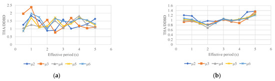
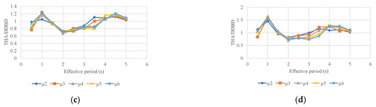
Figure 4.
Time-history analysis/DDBD displacement average ratio using approach 1 and a set of synthetic accelerograms: (a) EPP (r = 0), (b) bilinear (r = 0.2), (c) Takeda model (“narrow” type, α = 0.5, β = 0.0, r = 0.05), (d) Takeda model (“fat” type α = 0.3, β = 0.6, r = 0.05).
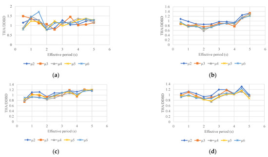
Figure 5.
Time-history analysis/DDBD displacement average ratio using approach 2 and a set of synthetic accelerograms: (a) EPP (r = 0), (b) bilinear (r = 0.2), (c) Takeda model (“narrow” type, α = 0.5, β = 0.0, r = 0.05), (d) Takeda model (“fat” type α = 0.3, β = 0.6, r = 0.05).
3.1.1. Approach 1
By analysing the graphs presented in Figure 4, it can be noticed that the displacement ratio obtained by using the equations proposed by Blandon and Priestley depends on the considered hysteretic model, on the ductility level, and on the effective period. When the value of the displacement ratio is higher than the unity, then:
It can be noticed that this is an underestimation of the equivalent damping obtained by using Equations (11)–(14). In this case, the formulation used to evaluate the equivalent viscous damping leads to smaller displacements than the ones obtained from nonlinear time-history analysis. It can be noted that the agreement is better for the models characterized by a lower hysteretic energy (see the Takeda “narrow” model in Figure 4c) where the average ratio is generally within ±15% of the unity. In general, it is not possible to identify a clear trend in the DR as a function of the ductility level, even if in Figure 4b–d it seems there is a lower dependency on ductility level than in Figure 4a. In the case of models characterized by a larger hysteretic energy, as in the case of the EPP model, the average values of the ratio are much greater than the other cases, up to twice the unity.
The results related to the elastic perfectly plastic hysteretic model presented in Figure 4a show, on average, high values for the DR with respect to the other hysteretic models, partially due to the post-yield stiffness ratio () [18]. For this model, the formulation proposed by Blandon and Priestley tends to provide DR values that are mostly higher than one for each ductility level and effective period. The DR trend for the bilinear model (Figure 4b) is quite uniform, especially for central periods (1.5–4 s) for all ductility levels. In the case of both Takeda models the trend is similar, with DR values of about 0.8 in the central region of periods (between 1.5 s and 3.5 s) and values larger than the unity outside this region. Between these two Takeda models, the Takeda “fat” provides larger values than the “narrow” outside the central region.
3.1.2. Approach 2
In this section the results of the analyses carried out by using approach 2, as explained in Section 2.2.3 of this paper, are reported. The verification procedure has been repeated by using the damping reduction factor η provided by EC8 [30] for the reduction in the elastic spectra in the application of DDBD.
By observing the results presented in the graphs reported in Figure 5, the use of approach 2 leads to smaller values of the displacement ratio than the ones obtained through approach 1. The results indeed show a closer approximation of the displacement ratio to the unitary value. In fact, the equations proposed by Blandon and Priestley have been formulated by reducing the elastic spectra in the DDBD procedure through the DRF η. In general, the use of this factor involves more conservative estimates of displacement demand, and then an underestimation of the damped spectra [40,41,42,43].
Also in this case, by examining the graphs in Figure 5, it is clear how the displacement ratio obtained by using the equations from Blandon and Priestley depends on the hysteretic model, on the ductility level, and on the effective period. As for approach 1, better results are obtained in the case of models characterized by lower hysteretic energy (as in the case of Takeda “narrow” model) where the average ratio is generally within ±10% of unity. In the case of the EPP model, the average values of ratios are always much higher, presenting values 60–70% higher than the unity. Similar to what has been observed for the results obtained by using approach 1, the elastic perfectly plastic model (Figure 5a) presents a noteworthy variety of DR values for all ductility levels and effective periods. The results related to the bilinear model presented in Figure 5b show quite uniform values for all ductility levels and periods, with DR values only being higher than one for longer periods (4.5–5 s). By analysing the two Takeda models, the trend is similar, with quite uniform values and an increasing tendency for longer periods. As for approach 1, the values obtained with Takeda “fat” seem larger than those obtained with Takeda “narrow”, even if these differences seem more evident for approach 1.
3.2. Calibration of Equivalent Viscous Damping Equations
In order to improve the results obtained in the last section, a calibration of the equivalent viscous damping equations has been performed, keeping the formal aspect of Equation (4) unchanged. This calibration has been carried out by considering different types of hysteretic models, ductility levels, and effective periods.
Therefore, four different sets of parameters have been derived (one for each hysteretic model). The maximum displacements in the SDOF systems have been estimated through nonlinear time-history analyses and through DDBD. A procedure has then been developed with the aim of minimizing the difference between the two values of displacements obtained.
Among the four parameters (a, b, c, d) used to characterize each hysteretic model, the b and c coefficients have been kept unchanged for each case (, ). Indeed, it has been shown that varying the hysteretic model does not significantly affect these parameters [18].
The calibration has been performed using the same twelve artificial ground motions defined in Section 2.2.3. As in the previous section, two approaches have been applied for the determination of the higher damped spectra in the DDBD procedure.
In approach 1 the spectra have been evaluated by using the Seismosignal software. In order to calibrate the parameters used in the viscous damping equations within the DDBD procedure, for each accelerogram and hysteretic model, an iterative process has been activated to obtain a value of the DR equal to one. In particular, the application of DDBD has been repeated by modifying the value of the equivalent viscous damping obtained by using Blandon and Priestley’s equations with prefixed a and d until a difference less than or equal to 3% has been reached between the DDBD and the displacement derived from the time-history analysis. The value related to this condition has then been computed for each pair and has been called .
In approach 2, an alternative methodology that considers the damping reduction factor , used to obtain the damped displacement spectra, has been proposed. By considering the latter approach, the design displacement in DDBD procedure has been computed as:
In order to obtain an equal displacement between the time-history analysis and the DDBD procedure, it has been assumed that:
In this way, it has been possible to obtain the value of as:
In both approaches, a different value of has then been derived for each ground motion. The average over all the twelve ground motions has then been determined (procedure of Section 2.2.1). For each hysteretic model, by considering the damping value , computed by using Blandon and Priestley’s [18] equations with prefixed a and d, the error in terms of difference between and , has been computed as:
This calculation has been repeated for all the considered ductility levels and effective period values (see Section 3.1), and the following error estimate has been derived as:
The error depends then only on the prefixed values of a and d. Therefore, the calibration involved the calculation of for several values of a and d: 500 values of a in the interval [1, 500], and 60 values of d in the interval [0.1, 6]. Finally, the values of a and d associated with the minimum , for all a and d, have been taken as the calibrated values.
Table 3 shows the proposed parameters calibrated by using approaches 1 and 2, compared with the one proposed by Blandon and Priestley [18].
Table 3.
Sets of parameters a and d in Equation (4) for each hysteretic model.
3.3. Verification of the Calibrated Parameters by Using Natural Accelerograms
In this section, a comparison between the use of the latter calibrated parameters (obtained through both approaches 1 and 2) and those proposed by Blandon and Priestley [18] is shown. With this aim, the verification algorithm described in Section 2.2.1 has then been applied. A set of fourteen natural accelerograms, divided into two main categories (far-field and near-field records) has been considered. The choice of these accelerograms has been made in order to take into account different types of ground motions by considering parameters such as the Arias intensity, the significant duration, and the PGA intensity. These ground motions, listed in Table 4, have been obtained from the PEER NGA Strong Motion Database [45], in NGA format.
Table 4.
Natural ground motions considered in the study.
The values shown in this section for each hysteretic model are the average results of fourteen different analyses each performed by using one of the ground motions listed in Table 4. As in Section 3.1 of this paper, the displacement ratio has been plotted (Figure 6 and Figure 7) against the effective period for different ductility levels.
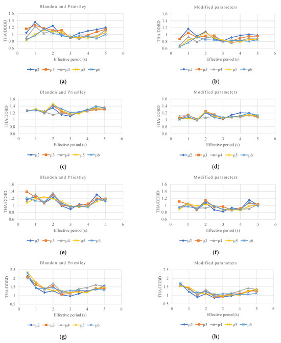
Figure 6.
Time-history analysis/DDBD displacement average ratio using approach 1 and a set of natural accelerograms: (a,b) EPP (r = 0), (c,d) bilinear (r = 0.2), (e,f) Takeda model (“narrow” type, α = 0.5, β = 0.0, r = 0.05), (g,h) Takeda model (“fat” type α = 0.3, β = 0.6, r = 0.05).
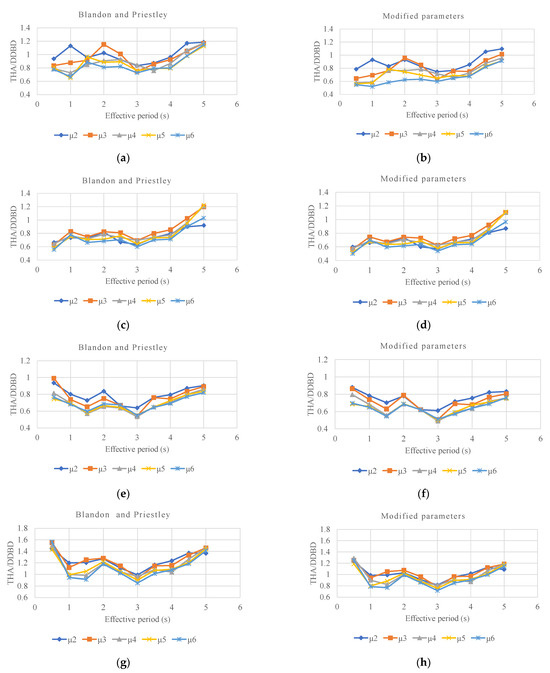
Figure 7.
Time-history analysis/DDBD displacement average ratio using approach 2 and a set of natural accelerograms: (a,b) EPP (r = 0), (c,d) bilinear (r = 0.2), (e,f) Takeda model (“narrow” type, α = 0.5, β = 0.0, r = 0.05), (g,h) Takeda model (“fat” type α = 0.3, β = 0.6, r = 0.05).
3.3.1. Approach 1
The results related to Blandon and Priestley’s parameters and to those calibrated in this study using approach 1 are presented in Figure 6. In general, it seems that the use of the parameters calibrated in this study have determined a reduction in the DR values in comparison to those obtained with Blandon and Priestley’s parameters. This reduction means a more conservative estimate of equivalent viscous damping. It is possible to notice how, for all the aforementioned hysteretic models, a decrease of up to 20% in the DR values can be obtained by using the calibrated values with respect to the parameters from the literature (Figure 6b,d,f,h). Moreover, it seems that the calibrated parameters have determined not only lower values than those provided by Blandon and Priestley, but also values closer to the unity in the period ranges in which the formulation with the original parameters provided values larger than the unity.
By analysing the graphs shown in Figure 6, it can be noticed that the agreement is better in the case of models characterized by lower hysteretic energy (i.e., bilinear and Takeda “narrow”) by using both the calibrated equations and those from the literature. Particularly noteworthy are the results related to the bilinear model (Figure 6c,d) where, excluding some intermediate period values, quite regular values of the DR for all ductility levels can be noted by using both the literature and the calibrated equivalent viscous damping equations. Blandon and Priestley’s parameters have provided, in the case of models characterized by greater hysteretic energy, as in the case of EPP (Figure 6a), an average ratio generally within ±40% of unity. For the two Takeda models, the “narrow” one (Figure 6e) presents an average ratio which differs generally from the unity by about ±20%. The results related to the Takeda “fat” model (Figure 6g) show DR values up to two times higher than one.
3.3.2. Approach 2
As in the case of approach 1, the results in Figure 7 show how the use of calibrated parameters leads to a significant decrease in the values of DR compared to those obtained by using Blandon and Priestley’s [18] equations. In the case of the bilinear model, it is possible to notice that the values of the displacement ratio (using Blandon and Priestley’s parameters) are substantially equal to one for most period values, with an average ratio within ±10% of the unity only for the effective period of 5 s. By using the parameters calibrated in this study, lower ratios have been obtained, with values slightly higher than the unity only for high periods. By analysing the results related to the Takeda “narrow” model, a uniform trend of the DR can be noted, with values almost constantly equal or lower than the unity, using both Blandon and Priestley’s parameters and the calibrated values. In the case of models characterized by greater hysteretic energy such as EPP and Takeda “fat” models, it is possible to find average values of DR that are slightly higher than the unity for some period values. By comparing the graphs obtained by using the DRF η and those obtained through approach 1, a general reduction in the DR values can be observed, both by using the parameters proposed by Blandon and Priestley and the calibrated ones.
For the models characterized by lower hysteretic energy and for intermediate periods (Figure 7) values lower than one have been derived with Blandon and Priestley’s parameters. In such cases the reduction determined with the calibrated parameters is associated with more conservative estimates.
3.4. Applications
The considered equivalent viscous damping formulations have been further tested by applying them for the design of a set of typical RC frames. In particular, the direct displacement-based design procedure has been applied to three RC frame structures by using the different equivalent viscous damping formulations relative to the Takeda “fat” model.
The considered equations are the one (Equation (22)) indicated in the Model Code 2009 [46], the one proposed by Blandon and Priestley [18] with its original parameters (Equation (23)), and the ones obtained at the end of the calibration procedure described in the present paper through approaches 1 and 2 (Equations (24) and (25)):
The structures designed through the DDBD procedure have then been modelled by using the finite element computer program SAP2000 [47]. Pushover and nonlinear time-history analyses have then been performed. The displacement and inter-storey drift profiles obtained through the DDBD procedure have been compared with the ones obtained through the nonlinear analyses.
In this study, the damped displacement spectra used in the DDBD procedure have been computed in two different ways, following approaches 1 and 2, described in Section 2.2.3. In particular, the equation proposed in the Model Code 2009 and the formulation presented by Blandon and Priestley, with the related parameters, have been applied with both of the approaches. Each set of parameters proposed in this paper has been applied with the approach used in the corresponding calibration.
3.4.1. Design Spectrum
The design spectrum has been defined according to Eurocode 8 [30] considering a soil type “C” and a peak ground acceleration of 0.407 g for a 10% probability of exceedance in 50 years. The displacement spectrum has been calculated from the acceleration spectrum by using the following expression:
For each of the considered frame structures, the DDBD procedure has been repeated six times, in relation to the three different equivalent viscous damping formulations (Equations (22)–(25)) and the two approaches illustrated in Section 2.2.3. Approach 1 involved the use of an average spectrum, computed over a set of seven different damped spectra, obtained with the Seismosignal software, considering the equivalent viscous damping values calculated through Equations (22)–(24). The seven accelerograms used in this phase have been artificially generated with the SIMQKE software [37] in order to be compatible with the considered Eurocode 8 design spectrum. In approach 2, the damped spectrum was obtained from the elastic spectrum reduced through the DRF provided by the Eurocode 8 [30]. In this approach, Equations (22), (23) and (25) have been used to compute the equivalent viscous damping index.
3.4.2. Frame Description
Three frames (Figure 8) with four, eight, and twelve storeys, characterized by a constant inter-storey height of 3.2 m and three bays, each 6 m in width, have been considered. The beams are rectangular, with a section characterized by a width and depth, respectively, of 30 and 50 cm for all of the storeys and all of the considered structures. The dimensions of the cross section of the rectangular columns are listed in Table 5. It has been assumed to have a concrete cylindrical compressive strength equal to 20 MPa and reinforced steel with a yield strength of 450 MPa. In order to model the inelastic behaviour of beams and columns, a concentred plasticity model has been implemented; the plastic hinges, located at the ends of each element, are characterized by a bilinear moment-rotation curve, defined by determining the yield and the ultimate bending moments and the corresponding chord rotations. Beam-type hinges characterized by the Takeda “fat” hysteretic model [48] have been used for all the structural elements.
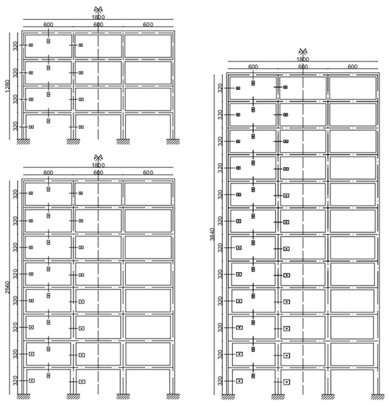
Figure 8.
Four, eight, and twelve-storey vertically regular RC frames (dimensions in cm).
Table 5.
Cross section dimensions of columns (dimensions in cm).
To determine the design actions on beams and columns, the DDBD has been applied according to the procedures reported in Section 3.4.1, considering the assumptions and the methods presented by Priestley et al. [8] and by the Model Code 2009 [46]. Specifically, the method based on equilibrium considerations, as described in [8], was used for determining the required moment capacities at potential hinge locations for the considered frames designed with the DDBD procedure. The results obtained for the RC frame structures designed by using the two approaches and the different equivalent viscous damping formulations described in Section 3.4.1 of this paper are listed below in Table 6 and Table 7.
Table 6.
DDBD parameters of frames designed with approach 1 and different equivalent viscous damping formulations.
Table 7.
DDBD parameters of frames designed with approach 2 and different equivalent viscous damping formulations.
3.4.3. Pushover Analyses
Pushover analyses were initially performed in order to compare the curves computed from the DDBD procedure (i.e., for the SDOF system) with the curves obtained with the adopted FEM computer program. According to the DDBD procedure, after modelling the equivalent SDOF system for each considered frame, the pushover curves have been computed, by using the yield and ultimate displacements and the design base shear (reported in Table 6 and Table 7).
The capacity curve of each MDOF frame has been obtained by performing a pushover analysis with the same distribution of lateral loads used in the DDBD procedure. The collapse point has been determined when the ultimate rotation in the first plastic hinge has been reached.
In order to compare directly, for each frame, the curves obtained through the DDBD procedure and the pushover analysis, a transformation from the curve of the MDOF system obtained with pushover analysis to the curve of the SDOF system has been necessary. This transformation is based on the computation of an equivalent displacement () of the MDOF system for each base shear value. In particular, for each step in the pushover analysis, knowing the displacement profile, it is possible to evaluate the equivalent displacement as:
The curves obtained from pushover analysis have then been linearized with the equal area criterion, keeping the same slope for the elastic range and the same ultimate displacement. These curves have been called linearized pushover curves (LPOC).
In Figure 9 the results related to the pushover analyses are presented, showing, in each case, the curves obtained for the structures designed with different equivalent viscous damping equations. In particular, the pushover curves are plotted in the base shear vs. equivalent SDOF displacement plane. For each considered frame, two graphs are reported. The first refers to the curves obtained using approach 1 (Figure 9a,c,e), with reference to the method for determining the damped spectra in the DDBD procedure, while the second has been obtained from the frames designed using approach 2 (Figure 9b,d,f).
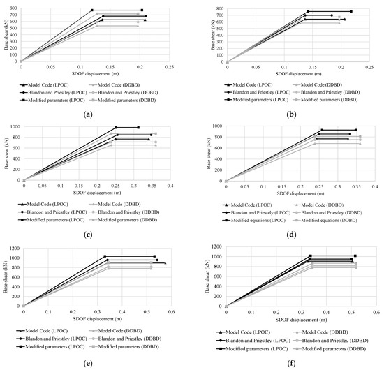
Figure 9.
Linearized pushover curves (LPOC) obtained for the four-storey (a,b), eight-storey (c,d) and twelve-storey (e,f) frames designed with three different damping equations (Model Code 2009, Blandon and Priestley, proposed parameters) and approach 1 (a,c,e) or approach 2 (b,d,f).
The results show a good correspondence between the pushover curves obtained with the FEM software and the DDBD procedure. In all of the analysed cases it can be noticed how the pushover curves from the FEM analyses provide slightly higher values (in terms of base shear) than the one obtained from the DDBD procedure. Moreover, the base shear presents higher values when the proposed equations calibrated in this work (with both the approach 1 and 2) are used, with respect to the values obtained by using the equations from the literature.
By analysing the results related to approach 1 in Figure 9a,c,e, it can be noticed that the curves related to the proposed parameters present higher stiffness values. This can be explained by the fact that the equations proposed by the Model Code and by Blandon and Priestley have been calibrated by using spectra reduced with the η parameter (approach 2, as explained in Section 2.2.3), while the proposed equations have been calibrated by using approach 1. Furthermore, in most cases the results related to approach 1 in comparison to approach 2 show a reduction in the ultimate displacement in all the frames, against an increase in stiffness and in maximum base shear.
It can be noted, in the case of approach 2 (Figure 9b,d,f), that the trend of the pushover curves related to the calibrated equations is more similar to those proposed by Blandon and Priestley [18].
3.4.4. Nonlinear Time-History Analyses
Nonlinear time-history analyses (NLTH) have been also performed on the considered frames by using the set of seven synthetic accelerograms presented in Section 3.4.1. In particular, as three frame structures with different number of storeys and six equivalent damping values considering two approaches and three different equivalent damping formulations (Equations (22)–(24) or (25)) have been taken into account, a total of 126 nonlinear time-history analyses have been run.
The results of time-history analyses have been used to assess the reliability of the design procedure based on the DDBD, by analysing the differences in terms of maximum displacements and inter-storey drifts. The design displacement profile, corresponding to the inelastic first mode shape at the design drift limit, has been determined by using the equation [46]:
where the term represents the design reduction factor. However, in the performed analyses, this factor has always been set equal to the unity, since also for the tallest frame the following result has been derived:
In this context, the DDBD displacement profile has been compared with the curve obtained by averaging the maximum displacement profiles computed through the time-history analyses for the seven ground motions. It can be observed that the displacement profile obtained from the DDBD procedure depends only on the storey height and the drift limit, differently from the profile obtained from NLTH.
In Figure 10, Figure 11 and Figure 12, the graphs (a) and (c) represent the design displacement profile of DDBD procedure and the averaged maximum displacements obtained from nonlinear time-history analyses for the frames designed using different equivalent viscous damping formulations and approaches 1 (a) or 2 (c). In graphs (b) and (d) the inter-storey drifts associated with the displacement profiles of graphs (a) and (c) are shown.
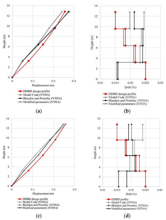
Figure 10.
Displacement and inter-storey drift average envelopes obtained with NLTH for the three four-storey frames designed with different damping equations (Model Code 2009, Blandon and Priestley, proposed parameters) and approach 1 (a,b) or 2 (c,d), compared with the DDBD design profile.
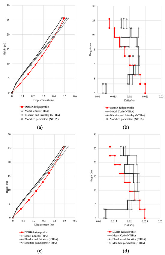
Figure 11.
Displacement and inter-storey drift average envelopes obtained with NLTH for the three eight-storey frames designed with different damping equations (Model Code 2009, Blandon and Priestley, proposed parameters) and approach 1 (a,b) or 2 (c,d), compared with the DDBD design profile.
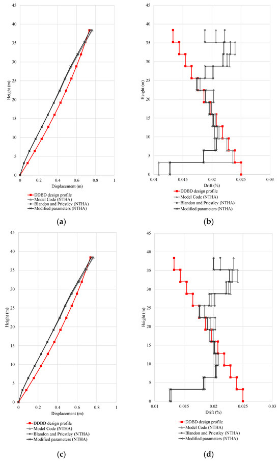
Figure 12.
Displacement and inter-storey drift average envelopes obtained with NLTH for the three twelve-storey frames designed with different damping equations (Model Code 2009, Blandon and Priestley, proposed parameters) and approach 1 (a,b) or 2 (c,d), compared with the DDBD design profile.
From the results reported in Figure 10, Figure 11 and Figure 12, it can be noticed that there is a good match between the displacement profiles obtained from the DDBD procedure and those from nonlinear time-history analyses. In particular, the set of displacement profiles obtained from time-history analyses generally presents an almost linear trend, representing a ductile collapse mechanism. It can be noted that, in most cases, the displacement of lower storeys computed from NLTH is lower than the design profile. This is probably due to the collapse mechanism obtained in NLTH, which is not always characterized by formation of plastic hinges in all base sections. In general, except the last storeys, the design DDBD displacement profile shows larger values than those from NLTH, showing that all the considered damping equations provides substantially conservative results. The displacement values obtained for the structures designed using the equivalent damping equation with the proposed parameters show similar or slightly lower values than other cases. This demonstrates the effectiveness of the equation with the proposed parameters too.
Concerning the inter-storey drifts, the mean values obtained from the time-history analyses are always lower than the 2.5% limit assumed in the design according to [46], and in most cases, the use of damping equations with the proposed parameters in the design provides lower drifts than those obtained by using the literature formulations, as shown in Table 8. On average, for the three considered structures, these reductions can be quantified as follows: when compared with the formulation of the Model Code, the maximum drift ratios obtained with the proposed formulations are reduced by approximately 10.5% and 7% for approach 1 and 2, respectively; when compared with the formulation of Blandon and Priestley, these reductions are approximately 8.5% and 4.5% for approach 1 and 2, respectively. For taller frames (Figure 12), it can be noticed that the upper part of the structure presents larger drifts in comparison with the design profile, due to the upper mode’s amplification [49], but always lower values than the maximum design drift of 2.5%.
Table 8.
Maximum inter-storey drift ratios (in percentage) obtained from nonlinear time-history analyses.
By observing the results shown in Figure 10a,b related to approach 1 for the four-storey frames, it can be noted how, by using the equations from the Model Code [46] and those by Blandon and Priestley [18], the displacement values in the first three storeys are lower than the ones provided by the DDBD procedure, contrary to the displacement value at the top level. By using the parameters proposed in this paper, a reduction in the top maximum displacement can, however, be noted. Concerning the inter-storey drifts, for the structures designed by using the damping equations from the literature, the drift values from NLTH are higher than those obtained from the DDBD design displacement profile at all storeys above the ground floor, but in all cases they are lower than the design value of 2.5%. Instead, by using the calibrated parameters to evaluate equivalent viscous damping, the drifts are lower than the ones obtained from the DDBD procedure for all the storeys, except for the top level.
In the case of approach 2 (Figure 10c,d), the same tendencies observed for approach 1 can be noted. However, in comparison with approach 1, the displacement values obtained with NLTH for the structures designed with literature damping equations are lower, while those for the structures designed with the calibrated parameters are slightly larger. Therefore, the difference observed between the different structures at the highest storeys are reduced passing from approach 1 to 2.
Similar results have been found for the eight-storey frames (Figure 11); by using the proposed parameters, both in approaches 1 and 2, a reduction in the maximum displacements of the upper storeys can be noticed. From the results related to the inter-storey drifts in Figure 11a,b, the drift values obtained through time-history analysis with the proposed parameters are lower than those of literature formulations. However, above the second storey, higher drift values than those obtained by using the DDBD procedure are obtained in both the approaches. The use of the proposed parameters provides a drift trend that better matches the DDBD one for the upper floors.
For the twelve-storey frames (Figure 12), results similar to the previous cases can be noted. In particular, the average maximum displacements obtained by using the modified parameters are lower than those provided by the literature ones. As concerns the inter-storey drifts, higher values than those obtained from DDBD can be observed in the upper part of the frame, contrary to the lower part which is characterized by smaller drifts.
4. Discussion
With respect to the existing literature, the work of Blandon and Priestley [18] has been considered as a reference point for the comparison and for developing the proposed formulations of the EVD. Specifically, for the SDOF systems, the analysis algorithm proposed by Blandon and Priestley has been used but, differently from [18], a larger set of accelerograms (twelve artificial ground motions compatible with the displacement design spectrum and related to different types of soil and different intensities) and a wider range of effective periods (0.5–5 s) have been considered. From the obtained results, it is possible to notice that, in various cases, the displacements provided by the time-history analyses are higher with respect to those obtained from the DDBD procedure, especially for the hysteretic models characterized by a high energy dissipation (e.g., EPP and Takeda “fat” models).
After the calibration of the proposed formulations of the EVD, the verification algorithm by Blandon and Priestley has been applied, and the results of these analyses have shown a reduction in the displacement ratio ( for most cases with respect to the values obtained through literature parameters. This tendency allowed to obtain results to be more conservative and closer to the unity in the ranges where the formulation with the original parameters provided displacement ratio values which were larger than the unity.
Referring to the RC frames designed with the DDBD procedure and to the capacity curves obtained through the pushover analyses, the results have shown a good correspondence between the pushover curves evaluated through the DDBD procedure and nonlinear analysis, as expected. Moreover, the results have shown different base shear values related to the considered equivalent viscous damping formulations. In particular, more conservative values have been obtained by using the proposed set of parameters. The good match between each pair of curves obtained from the DDBD and the software analysis is due to the effectiveness of the DDBD design procedure.
Referring to the RC frames designed with the DDBD procedure and to the nonlinear time-history analyses performed, the results have shown that the use of the calibrated parameters have determined more conservative results, for both of the considered approaches in terms of design base shear and maximum drift from NLTH. By analysing the results related to the inter-storey drifts, it has been noticed that all the equivalent viscous damping formulations have determined values below the design drift limit, for every frame considered. Moreover, the inter-storey drifts obtained for the frames designed with the proposed parameters show lower values than those for the frames designed through literature formulations, and closer to the values of the design profile. Similarly, the average displacement profiles obtained from time-history analyses for the frames designed with the calibrated parameters match the design displacement profile better.
5. Conclusions
In this paper, approaches for estimating the equivalent viscous damping of RC frame buildings have been proposed. This has been carried out by maintaining the structure of the original equation proposed by Blandon and Priestley [18] but varying the coefficients of the equation through a calibration procedure. Compared with the work of Blandon and Priestley [18], a larger set of synthetic accelerograms, related to different types of soil and different intensities, and a wider range of the effective periods have been considered. In particular, two different sets of parameters have been proposed: the first usable in the case of spectra obtained numerically (approach 1) and the second in the case of code-based spectra and damping modification factor (approach 2). The calibration procedure has been carried out by considering four hysteretic models, ten period values, six ductility levels, and a set of twelve synthetic ground motions. The first verification to show the superior performance of the proposed approaches has been carried out by considering SDOF systems and fourteen natural ground motions.
In order to investigate the performance of calibrated parameters in the design practice, three multi-storey reinforced-concrete frames with a different number of storeys have been designed with the DDBD procedure. For each case, the equivalent viscous damping index has been calculated by using three different formulations, including the sets of parameters proposed in this paper, and two different approaches to provide the damped displacement spectra (approach 1 and 2). Afterwards, the capacity curves have been obtained through pushover analyses performed on the frames designed with different equivalent viscous damping formulations. Finally, nonlinear time-history analyses, performed by using a set of seven synthetic accelerograms compatible with the considered design spectrum, have been run. The displacement profile obtained using DDBD and the averaged maximum displacements obtained from the nonlinear analyses have been compared for each frame (designed with a different equivalent viscous damping formulation). For the case studies, the results have shown that the use of the calibrated parameters (for both the considered approaches) have determined more conservative results, in terms of design base shear and maximum drift from NLTH. Moreover, the average displacement profiles and the inter-storey drifts obtained from time-history analyses for the frames designed with the calibrated parameters match the design profile better.
Author Contributions
Conceptualization, L.L. and P.P.D.; methodology, L.L.; software, C.B., S.Q. and L.L.; investigation, C.B. and L.L.; writing—original draft preparation, C.B. and L.L.; writing—review and editing, L.L., S.Q. and G.B.; visualization, C.B., S.Q., L.L. and G.B.; supervision, L.L. and P.P.D. All authors have read and agreed to the published version of the manuscript.
Funding
This research received no external funding.
Data Availability Statement
The raw data supporting the conclusions of this article will be made available by the authors on request.
Conflicts of Interest
The authors declare no conflicts of interest.
References
- Priestley, M.J.N. Myths and Fallacies in Earthquake Engineering—Conflicts between Design and Reality. Bull. N. Z. Soc. Earthq. Eng. 1993, 26, 329–341. [Google Scholar]
- Priestley, M.J.N. Performance based seismic design. In Proceedings of the 12th World Conference on Earthquake Engineering, Auckland, New Zealand, 30 January–4 February 2000. paper no. 2831. [Google Scholar]
- Priestley, M.J.N. Myths and Fallacies in Earthquake Engineering, revisited. The 9th Mallet Milne Lecture; IUSS Press: Pavia, Italy, 2003. [Google Scholar]
- Sullivan, T.J.; Calvi, G.M.; Priestley, M.J.N.; Kowalsky, M.J. The limitations and performances of different displacement based design methods. J. Earthq. Eng. 2003, 7, 201–241. [Google Scholar] [CrossRef]
- Muljati, I.; Asisi, F.; Willyanto, K. Performance of force based design versus direct displacement design in predicting seismic demands of regular concrete special moment resisting frames. In Proceedings of the 5th International Conference of Euro Asia Civil Engineering Forum, Surabaya, Indonesia, 15–18 September 2015; pp. 1050–1056. [Google Scholar]
- Castellanos, H.; Ayala, A.G. Trends in the displacement-based seismic design of structures, Comparison of two current methods. In Proceedings of the 15th World Conference on Earthquake Engineering, Lisboa, Portugal, 24–28 September 2012. 10p. [Google Scholar]
- Panagiotakos, T.B.; Fardis, M.N. Deformation-controlled earthquake-resistant design of RC buildings. J. Earthq. Eng. 1999, 3, 495–518. [Google Scholar] [CrossRef]
- Priestley, M.J.N.; Calvi, G.M.; Kowalsky, M.J. Displacement-Based Seismic Design of Structures; IUSS Press: Pavia, Italy, 2007. [Google Scholar]
- Shibata, A.; Sozen, M.A. Substitute-structure method for seismic design in R/C. J. Struct. Div. (ASCE) 1976, 102, 1–18. [Google Scholar] [CrossRef]
- Sullivan, T.J.; Calvi, G.M.; Priestley, M.J.N. Initial stiffness versus secant stiffness in displacement based design. In Proceedings of the 13th World Conference on Earthquake Engineering, Vancouver, BC, Canada, 1–6 August 2004. paper no. 2888. [Google Scholar]
- Dwairi, H.M.; Kowalsky, M.J.; Nau, J.M. Equivalent Damping in Support of Direct Displacement-Based Design. J. Earthq. Eng. 2007, 11, 512–530. [Google Scholar] [CrossRef]
- Kumbhar, O.G.; Kumar, R.; Farsangi, E.N. Investigating the efficiency of DDBD approaches for RC buildings. Structures 2020, 27, 1501–1520. [Google Scholar] [CrossRef]
- Landi, L.; Saborio-Romano, D.; Welch, D.P.; Sullivan, T.J. Displacement-based simplified seismic loss assessment of post-70s RC buildings. J. Earthq. Eng. 2020, 24 (Suppl. S1), 114–145. [Google Scholar] [CrossRef]
- Sullivan, T.J.; Saborio-Romano, D.; O’Reilly, G.J.; Welch, D.P.; Landi, L. Simplified pushover analysis of moment resisting frame structures. J. Earthq. Eng. 2021, 25, 621–648. [Google Scholar] [CrossRef]
- Jacobsen, L.S. Steady forced vibration as influenced by damping. Trans. ASME 1930, 52, 169–181. [Google Scholar]
- Miranda, E.; Ruiz-Garcia, J. Evaluation of the approximate methods to estimate maximum inelastic displacement demands. Earthq. Eng. Struct. Dyn. 2002, 31, 539–560. [Google Scholar] [CrossRef]
- Priestley, M.J.N.; Grant, D.N. Viscous Damping in Seismic Design and Analysis. J. Earthq. Eng. 2005, 9, 229–255. [Google Scholar] [CrossRef]
- Blandon, C.A.; Priestley, M.J.N. Equivalent viscous damping equations for direct displacement based design. J. Earthq. Eng. 2005, 9, 257–278. [Google Scholar] [CrossRef]
- Tarawneh, A.; Majdalaweyh, A.; Dwairi, H. Equivalent viscous damping of steel members for direct displacement based design. Structures 2021, 33, 4781–4790. [Google Scholar] [CrossRef]
- Sirotti, S.; Aloisio, A.; Pelliciari, M.; Briseghella, B. Empirical formulation for the estimate of the equivalent viscous damping of infilled RC frames. Eng. Struct. 2023, 288, 116196. [Google Scholar] [CrossRef]
- Mohebkhah, A.; Tazarv, J. Equivalent viscous damping for linked column steel frame structures. J. Constr. Steel Res. 2021, 179, 106506. [Google Scholar] [CrossRef]
- Farahani, S.; Akhaveissy, A.H.; Damkilde, L. Equivalent viscous damping for buckling-restrained braced RC frame structures. Structures 2021, 34, 1229–1252. [Google Scholar] [CrossRef]
- Augusto, H.; Castro, J.M.; Rebelo, C.; da Silva, L.S. Ductility-equivalent viscous damping relationships for beam-to-column partial-strength steel joints. J. Earthq. Eng. 2019, 23, 810–836. [Google Scholar] [CrossRef]
- Gu, A.; Shen, S.D. The influences of equivalent viscous damping ratio determination on direct displacement-based design of un-bonded post-tensioned (UPT) concrete wall systems. Smart Struct. Syst. 2022, 30, 627–637. [Google Scholar]
- Landi, L.; Tardini, A.; Diotallevi, P.P. A procedure for the displacement-based seismic assessment of infilled RC frames. J. Earthq. Eng. 2016, 20, 1077–1103. [Google Scholar] [CrossRef]
- Aloisio, A.; Alaggio, R.; Fragiacomo, M. Equivalent viscous damping of cross-laminated timber structural archetypes. J. Struct. Eng. 2021, 147, 04021012. [Google Scholar] [CrossRef]
- Dong, W.; Li, M.; Sullivan, T.; MacRae, G.; Lee, C.L.; Chang, T. Direct displacement-based seismic design of glulam frames with buckling restrained braces. J. Earthq. Eng. 2023, 27, 2166–2197. [Google Scholar] [CrossRef]
- Merino, R.J.; Perrone, D.; Filiatrault, A. calibrated equivalent viscous damping for direct displacement-based seismic design of suspended piping trapeze restraint installations. J. Earthq. Eng. 2022, 26, 8063–8091. [Google Scholar] [CrossRef]
- Merino, R.J.; Gabbianelli, G.; Perrone, D.; Filiatrault, A. Calibrated equivalent viscous damping for direct displacement based seismic design of pallet-type steel storage racks. J. Earthq. Eng. 2023, 27, 1012–1046. [Google Scholar] [CrossRef]
- EN 1998-1; Eurocode 8. Design of Structures for Earthquake Resistance—Part 1: General Rules, Seismic Actions and Rules for Buildings. European Committee for Standardization: Brussels, Belgium, 2005.
- Rosenblueth, E.; Herrera, I. On a kind of hysteretic damping. J. Eng. Mech. Div. 1964, 90, 37–48. [Google Scholar] [CrossRef]
- Gulkan, P.; Sozen, M. Inelastic response of reinforced concrete structures to earthquake motions. ACI J. Proc. 1974, 71, 604–610. [Google Scholar]
- Iwan, W.D.; Gates, N.C. The effective period and damping of a class of hysteretic structures. Earthq. Eng. Struct. Dyn. 1979, 8, 199–211. [Google Scholar] [CrossRef]
- Kowalsky, M.J. Displacement-Based Design—A Methodology for Seismic Design Applied to RC Bridge Columns. Master’s Thesis, University of California, Los Angeles, CA, USA, 1994. [Google Scholar]
- Dwairi, H.; Kowalsky, M. Investigation of Jacobsen’s equivalent viscous damping approach as applied to displacement based design. In Proceedings of the 13th World Conference on Earthquake Engineering, Vancouver, BC, Canada, 1–6 August 2004. paper no. 228. [Google Scholar]
- Otani, S. Hysteresis models of reinforced concrete for earthquake response analysis. J. Fac. Eng. 1981, XXXVI, 407–441. [Google Scholar]
- Gelfi, P. SIMQKE_GR, Version 2.7 (Software). Available online: https://gelfi.unibs.it/software/simqke/simqke_gr.htm (accessed on 3 March 2024).
- Zaharia, R.; Taucer, F. Equivalent Period and Damping for EC8 Spectral Response of SDOF Ring-Spring Hysteretic Models; JRC Scientific and Technical Reports; Institute for the Protection and Security of the Citizen, European Commission: Luxembourg, 2008. [Google Scholar]
- Seismosoft. SeismoSignal—A Computer Program to Process Strong-Motion Data (Software). 2016 Version. Available online: http://www.seismosoft.com (accessed on 3 March 2024).
- Benahmed, B.; Hammoutene, M.; Cardone, D. Effects of damping uncertainties on damping reduction factors. Period. Polytech. Civ. Eng. 2017, 61, 341–350. [Google Scholar] [CrossRef][Green Version]
- Heng, L.; Chen, F. Damping modification factors for acceleration response spectra. Geod. Geodyn. 2017, 8, 361–370. [Google Scholar]
- Cardone, D.; Dolce, M.; Rivelli, M. Evaluation of reduction factors for high-damping design response spectra. Bull. Earthq. Eng. 2009, 7, 273–291. [Google Scholar] [CrossRef]
- Sheikh, M.N.; Tsang, H.; Yaghmaei-Sabegh, S.; Anbazhagan, P. Evaluation of damping modification factors for seismic response spectra. In Proceedings of the Australian Earthquake Engineering Society Conference 201, Hobart, Australia, 15–17 November 2013; pp. 1–13. [Google Scholar]
- Charney, F.A. Nonlin V8.00 (Software); Advanced Structural Concepts Inc.: Blacksburg, VA, USA, 2010. [Google Scholar]
- Pacific Earthquake Engineering Research Center. PEER NGA Database. 2013. Available online: https://ngawest2.berkeley.edu/ (accessed on 3 March 2024).
- Calvi, G.M.; Sullivan, T.J. A Model Code for the Displacement-Based Seismic Design of Structures; IUSS Press: Pavia, Italy, 2009. [Google Scholar]
- SAP2000 Software, Version 24; Computers and Structures, Inc.: Berkeley, CA, USA, 2022.
- Takeda, T.; Sozen, M.; Nielsen, N. Reinforced concrete response to simulated earthquakes. ASCE J. Struct. 1970, 96, 2557–2573. [Google Scholar] [CrossRef]
- Pettinga, J.D.; Priestley, M.J.N. Dynamic behaviour of reinforced concrete frames designed with direct displacement-based design. J. Earthq. Eng. 2005, 9, 309–330. [Google Scholar] [CrossRef]


Disclaimer/Publisher’s Note: The statements, opinions and data contained in all publications are solely those of the individual author(s) and contributor(s) and not of MDPI and/or the editor(s). MDPI and/or the editor(s) disclaim responsibility for any injury to people or property resulting from any ideas, methods, instructions or products referred to in the content. |
© 2024 by the authors. Licensee MDPI, Basel, Switzerland. This article is an open access article distributed under the terms and conditions of the Creative Commons Attribution (CC BY) license (https://creativecommons.org/licenses/by/4.0/).