Predicting the Displacement Variation of Rehabilitated Foundation of Onshore Wind Turbines Using Machine Learning Models

Abstract

The rehabilitation of wind turbine foundations after damage is increasingly common. However, limited research exists on the deformation of wind turbine foundations after rehabilitation. Artificial intelligence methods can be used to analyze future deformation state and predict post-rehabilitation deformation of foundations. This paper focuses on analyzing the stability of damaged wind turbine foundations after rehabilitation, as well as establishing and evaluating machine learning models. Specifically, Decision Tree (DT), Extreme Gradient Boosting (XGB), Support Vector Regression (SVR), and Long Short-Term Memory Network (LSTM) models are utilized to predict the vertical displacement of the rehabilitated foundation. Hence, the stability of the rehabilitated foundation is discussed in correlation with the measured wind speed, based on the foundation vertical displacement data. During the development of the machine learning model, the most suitable combination of hyperparameters is determined. The prediction performance of the SVR and LSTM models, which exhibit good performance, is compared to further evaluate their effectiveness. Furthermore, the models are analyzed and validated. The results indicate that the vertical displacements of the rehabilitated foundations gradually get close to a state of steady fluctuation over time. The SVR model is identified as the most effective in predicting the vertical displacements of wind turbine foundations after rehabilitation. This study aims to analyze and predict the vertical displacement of wind turbine foundations after rehabilitation based on extensive field monitoring data and powerful machine learning models.

1. Introduction

Wind power has emerged as a critical component of the future energy landscape. Simultaneously, it plays a pivotal role in accelerating the adjustment of the Chinese energy structure and achieving the ambitious goal of carbon neutrality by 2060 [1]. Due to the relatively late development of the Chinese wind power industry, several associated technologies exhibit noticeable hysteresis phenomena, including foundation fatigue damage [2,3] and the cracking of foundation ring concrete gap [4].

Given these challenges concerning wind turbine foundations, research on the mechanisms of foundation damage and rehabilitation techniques for damaged foundations has attracted growing attention from scholars. Guo et al. [5] discovered that torque load is most sensitive to changes in bottom flange size but less responsive to variations in the buried depth of the foundation ring or the strength of the foundation concrete. Velarde et al. [6] investigated the sensitivity of fatigue load for a 5 MW offshore wind turbine installed on a gravity base with respect to major structural, geotechnical, and marine parameters. They found that turbulence intensity and wave load uncertainty significantly influence fatigue load uncertainty, while soil property uncertainties exhibit nonlinear or interactive behavior. Amponsah et al. [7] proposed an analytical expression for the ultimate bending moment bearing capacity based on stress distribution and failure mode under observed ultimate loads for embedded steel ring-foundation connections. McAlorum et al. [8] employed an ultra-long fiber optic strain sensor to monitor crack development and changes in foundation concrete over time. Sun et al. [9] suggested using finite element method simulations to compare the effectiveness of different reinforcement schemes and determine the best method during the reinforcement design process.

In summary, research methods for wind turbine foundation deformation mainly focus on numerical simulation, which has drawbacks such as lengthy modeling time, complex analysis, and limited simulation applicability. In recent years, with the continuous advancement of artificial intelligence, machine learning models have been applied in finance, healthcare, transportation, environmental research, and other fields [9,10,11]. There is also abundant research on the application of machine learning models for prediction in the civil engineering industry, such as the seismic damage assessment of structures and analysis of material performance indicators [12,13]. Of course, in geotechnical engineering problems, machine learning is used to predict ground settlement in tunnel excavation and pipeline excavation instead of simulation [14,15]. Machine learning has been extensively studied in foundation settlement methods. Samui [16] used support vector machines to predict settlement in and out of shallow foundations with cohesionless soils, and concluded that SVM can serve as a practical tool for predicting foundation settlement. Scott Kirts et al. [17] also utilized support vector machines to make pertinent predictions of foundation settlement and demonstrated positive outcomes. In addition to the SVM method, Raja et al. [18] employed the Multivariate Adaptive Regression Splines (MARS) model to predict the deformation of reinforced foundations, while Deng et al. [19] proposed a prediction interval for the settlement of building foundations using an Extreme Learning Machine (ELM). Moreover, artificial neural networks are commonly employed in foundation settlement studies [20]. Currently, numerous studies have focused on the health monitoring of wind turbine foundations [21,22]. However, few studies have utilized machine learning models to predict foundation deformation under cyclic dynamic loads following the rehabilitation of fan foundations in mountainous areas. The applicability of machine learning models to predict wind turbine foundation deformation post-rehabilitation remains uncertain.

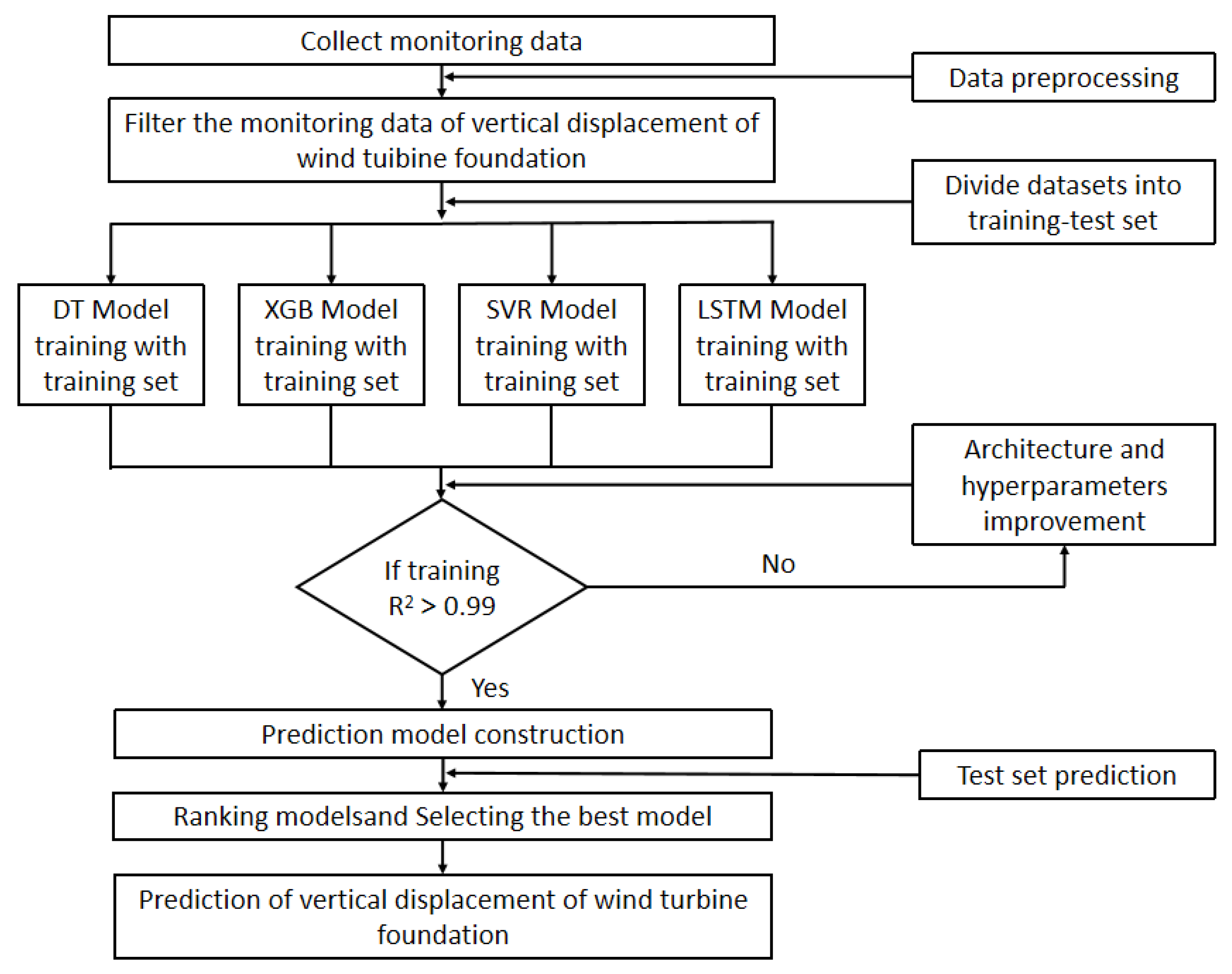
This study primarily analyzes the stability of damaged wind turbine foundations after rehabilitation and the predictive efficacy of machine learning on future foundation deformation. Firstly, the field deformation data following the rehabilitation of the mountainous wind turbine foundation are analyzed, and the stability of the wind turbine foundation deformation after rehabilitation is discussed. Subsequently, we investigate the applicability of machine learning in predicting wind turbine foundation displacement, establish a prediction model for wind turbine foundation vertical displacement deformation, assess the predictive performance of four machine learning models, and employ the best model to predict wind turbine foundation displacement. Furthermore, machine learning models are explored for the long-term prediction of wind turbine foundation deformation. The practical significance lies in the capability of the constructed model to accurately predict the vertical displacement of wind turbine foundations, offering data support for subsequent maintenance and serving as a reference for monitoring and predicting foundation deformations after rehabilitation.

2. Engineering Example Analysis

2.1. Project Profile

The wind farm comprises 24 wind turbines and is situated on a ridge along the northern border between Yazi Town, Lushan City, and Muping District, Yantai City. The ground elevation ranges from 315.00 m to 317.00 m, with the terrain slope ranging from 5° to 20°, and the hillside terrain slope generally ranging from 15° to 30°. The site plan is shown in Figure 1. The geological investigation revealed that the stratum lithology comprises weak gneissic medium-grained and medium–fine-grained monzonitic granite, with Quaternary deposits primarily composed of clayey silt, gravelly sandy clay, sandy silt with gravel, and subsoil containing sand, gravel, rubble, and plant roots. The wind turbine foundation system consists of secondary grouted micropiles and footings. The wind turbine foundation structure and strata section are illustrated in Figure 2. The wind farm was commissioned in November 2013 and subsequently connected to the grid. During early 2021 maintenance of the wind turbines on the project, more than 180 internal anchors and over 20 external anchors were found broken, with the number of fractures increasing, as depicted in Figure 3. Additionally, radial and circumferential crack fractures were observed on the surfaces of the turbine foundations.

Due to the potential safety hazards posed by the foundation issues, an experimental study was undertaken to rehabilitate and retrofit the foundation of turbine #22, which is located under favorable construction conditions. The specific rehabilitation process is described in Section 2.2.

2.2. Rehabilitation Operations

The foundation was optimized to deal with the three damaged stress components, rock anchors, foundation plate, and L-flange connection anchor bolts, so that they could meet the foundation stress requirements. For the outer ring anchors and foundation slabs, enlarged and thickened foundation slabs were used to improve the self-weight and overturning resistance of the foundations, while at the same time repairing the grade of the foundations themselves and reducing the tensile forces transmitted to the outer ring anchors. At the same time, by increasing the number of anchor rods, the length of the plate span reduces, thus reducing the internal force of the foundation plate. For the high-strength anchor bolts of the tower tube, the welding nail solution is adopted on the surface of the tower tube, connecting the outer concrete of the tower tube with the old foundation, so that the welding nail can bear the load and transfer it to the foundation. In this case, the foundation is connected to the tower by welded studs, and the L-flange connection anchor bolts are discarded. Figure 4 shows the #22 foundation modification project.

2.3. Measuring Point Position

To evaluate the effectiveness of the recommended foundation rehabilitation program, a static level gauge was used to monitor the deformation of the rehabilitated foundation of wind turbine #22. A complimentary fully automatic wireless data acquisition device was utilized to continuously collect deformation data and transmit it to a cloud storage platform. To ensure uninterrupted sensor operation throughout the year, an antifreeze solution was injected into the instrument. The working principle of the static liquid level gauge is to calculate vertical displacement changes by measuring the height of the liquid level changes at each measuring point. Suppose there are $n$ measuring points, point #1 is the reference point. When the observed object has uneven settlement, the distance between the liquid surface in the container of each measuring point and the installation elevation is set as $h_{k1}$… $h_{ki}$… $h_{kn}$ ($i$, $n$ is the test point code, $k$ is the test run code). At this point, it can be obtained that $h_{ki}-h_{k1}$ is the displacement of point $i$ in the k-th measurement with respect to horizontal point 1, and $h_{ki}-h_{ki-1}$ is the displacement of the liquid level sensor at point $i$ in the k-th measurement with respect to the previous time. Following the rehabilitation of wind turbine #22, four measurement points were subsequently installed on the foundation’s surface, as depicted in Figure 5.

It should be noted that Point 1 serves as the reference point. Considering that the static level gauge principle involves measuring the difference in liquid levels between the monitoring points and the reference point, the location of the liquid reservoir box needs to be higher than all the measurement points. Therefore, as shown in Figure 6, the reference point is placed on one side of the turbine switchboard foundation and connected to the switchboard foundation by a stainless-steel frame to create a certain level difference. As the distribution box has been used for many years, it can be assumed that the settlement at P-1 has reached a stable state.

2.4. Measured Data Analysis

The modifications to the wind turbine foundations were completed in early July, and on 22 July 2020, the installation of the deformation monitoring sensors was completed. Monitoring began immediately after the installation was completed. The site wind speed, turbine revolution, and foundation vertical displacement monitoring data from the start of monitoring until 31 October 2020, are shown in Figure 7.

As can be seen in Figure 7, the wind load at the site where the wind turbine is located peaked on 29 July 2020, the 7th day of monitoring, and due to the response to the wind load, the foundation deformation at all the measurement points showed a significant stepwise decrease on this day, with an average decrease of about −1.5 mm. Due to the circulation wind loads, the vertical displacements of the foundations showed significant fluctuations, ranging from 1 mm to −3 mm around the stabilized values. From 29 July to 19 September 2020, when the wind turbine was changed from the shutdown condition to the operation condition and the turbine speed fluctuated steadily, the vertical displacements at all measured points of the turbine foundation showed a slight upward trend. But the overall cumulative rebound phenomenon was not obvious, which indicated that the rehabilitation of the wind turbine foundation was obvious to achieve the constraints on the foundation.

During the period from 19 September to 21 September 2020, with the sustained peak wind loads and the turbine on condition, the monitoring results of all the measurement points showed a significant stepwise decrease with an average decrease of about −2.0 mm, which was the most significant decrease in foundation deformation in this timeframe. At the same time, there was a significant subsidence of the wind turbine foundation when the wind speed reached its peak.

From 22 September to 19 October 2020, the monitoring results at all points showed a slight downward trend with a cumulative deformation of about −1 mm. During this period, the wind speed again showed two peaks of wind loads, and the foundation also showed obvious subsidence phenomenon but immediately lifted to the normal zone as the wind speed decreased, indicating that the foundation deformation of the rehabilitated wind turbine has stabilized after cyclic wind loads. From 19 October 2020, the foundation deformation under cyclic wind load showed regular fluctuation within the range of −1.5 mm to −6.5 mm, and the foundation vertical displacement and deformation tended to stabilize, indicating that the wind turbine foundation rehabilitation scheme was successful.

The deformation of the rehabilitated foundation was found to be capable of relatively low fluctuations within a certain range. The cumulative deformation effect is found to be insignificant. Despite experiencing deformation under the working conditions of the wind turbine and cyclic wind loading, the rehabilitated foundation demonstrates a commendable ability to maintain a stable state. The above results show that the wind turbine foundations can improve the foundation bearing capacity and reduce the foundation deformation caused by cyclic loading after being strengthened by the method in this paper.

2.5. Modeling Process

In order to clearly represent the future change of wind turbine foundation after rehabilitation, this paper constructs a prediction model of vertical displacement change of wind turbine foundation through four kinds of machine learning methods to realize the prediction and research of future state of wind turbine foundation after rehabilitation.

Initially, wind farm foundation monitoring data are collected and pre-processed, involving cleaning and noise reduction. Subsequently, all monitoring data regarding the vertical displacement of wind turbine foundation are selected. The dataset is divided into training and test sets, comprising 80% and 20%, respectively, and used to train the model. The four machine learning models are initially constructed to train the vertical displacement of the wind turbine foundation, and are screened and parameter-optimized based on the performance of the models in the training set. Subsequently, the performance scores of the four machine learning models in the test set are statistically ranked, and the most suitable vertical displacement prediction model for the rehabilitated wind turbine foundation is derived through comparative analysis. Finally, the vertical displacement of the wind turbine foundation is predicted, with the flowchart of the model construction depicted in Figure 8.

3. Model Design

To accurately predict foundation deformation patterns under cyclic loading and assess the effectiveness of repair options, we conducted an in-depth analysis of the applicability of machine learning models in predicting the foundation displacement deformations induced by wind turbines. Subsequently, several wind turbine foundation vertical displacement prediction models were constructed for this project. The researchers chose four different models for modeling and analysis, including Decision Tree (DT), Extreme Gradient Boosting (XGB), Support Vector Regression (SVR), and Long Short-Term Memory Network (LSTM), and compared their performance.

3.1. Model Theory

(1)

DT Model. The Decision Tree model consists of a root node, internal decision nodes, and terminal leaf nodes [23,24]. Figure 9 shows the tree structure with a depth of 3. The principle of the model is to learn the classification of the data in the training set and get a set of classification rules suitable for the dataset, and classify the data.

(2)

XGB Model. The Extreme Gradient Boosting model is an improved model of gradient boosting regression trees, in which regularization is introduced to reduce the complexity of the trees and obtain better model performance. The model established in this paper is the CART regression tree model [25,26].

(3)

SVR Model. The Support Vector Regression model is derived from the support vector machine classification model. The main principle is to map a low-dimensional nonlinear data set to a high-dimensional space using a nonlinear function and then perform linear regression in the high-dimensional space. It constructs an optimal hyperplane that minimizes the distance between the data samples and the hyperplane, thereby solving the problem of linear inseparability in the original space [27,28,29]. Suppose the sample data set is $D=\{(x_i,y_i),i=1,2,\dots ,n\}$, $x_i$ is the input of the model and $y_i$ is the output of the model, $x_i,y_i\in R^m$. The sample data are mapped to a high-dimensional linear space with a nonlinear mapping $\phi \left(x\right)$ as follows:

$$f\left(x\right)=\omega \phi \left(x\right)+b$$

(1)

where $f\left(x\right)$ is the predicted value of the regression function, and $\omega$ and $b$ are the target parameters.

In order to adjust the prediction effectiveness and efficiency of the SVR model, the tolerance $\epsilon$ introduced to the SVR has a certain fault-tolerance ability, as shown in Figure 10. In order to solve the objective parameters $\omega$ and $b$, the problem is transformed into an optimization solution,

$$\left\{\begin{array}{c}\mathrm{e}(x,y,f)=\max (0,|y-f(x)-\epsilon |)\\ \min \frac{1}{2}||\omega |{|}^2+C{\displaystyle \sum _{i=1}^n({\xi }_i+{\xi }_i^{*})}\\ ({\omega }^T{x}_i+b)-y_i\le \epsilon +{\xi }_i,i=1,2,\dots ,n\\ y_i-({\omega }^T{x}_i+b)\le \epsilon +{\xi }_i^{*},i=1,2,\dots ,n\end{array}\right.$$

(2)

where $\epsilon$ is the insensitivity coefficient; $C$ is the penalization factor; ${\xi }_i$ and ${\xi }_i^{*}$ are both the slack variables.

Introducing the Lagrangian function to obtain the dyadic model solution, the final model solution can be obtained as

$$f(x)={\displaystyle \sum _{i=1}^n({\alpha }_i^{*}+{\alpha }_i)}K(x,x_i)$$

(3)

where $a_i^{*}$ and $a_i$ are Lagrange multipliers and $K(x,x_i)$ is the kernel function.

(4)

LSTM Model. The Long Short-Term Memory Network model is established to solve the short-term memory problem in recursive neural network models. The cell unit mainly consists of a forget gate, an input gate, an output gate, and a cell state chain [30,31,32]. The “gate” regulates the flow of information through internal control, and the cell state acts as a conveyor belt for information transmission between cell units. Figure 11 shows a single cell of LSTM, where $X_t$ represents the input information at time $t$, Tanh and $\sigma$ represent the hyperbolic tangent function and Sigmoid function, $C_t$ and $H_t$ represent the cell state and hidden state at time $t$. The principle of propagation in a single LSTM cell: first discards irrelevant information through the forget gate, then updates the required information through the input gate, and finally outputs the designated information through the output gate. The main computational process of the memory cell is as follows:

The genetic gate is cellular selection of informative data for oblivious computation, such as Equation (4).

$$f_t=\sigma (W_f\cdot [X_t,h_{t-1}]+b_f)$$

(4)

where $\sigma$ is the Sigmoid activation function, $b_f$ is the threshold of the forgetting gate, and $W_f$ is the weight of the forgetting gate.

The two parts of the output in the input gate are updated, as in Equations (5) and (6).

$$i_t=\sigma (W_i\cdot [x_i,h_{i-1}]+b_i)$$

(5)

$${\tilde{c}}_t=\tanh (W_0\cdot [x_i,h_{i-1}]+b_c)$$

(6)

where $W_i$, $W_0$, $b_i$ and $b_c$ are the weights and thresholds corresponding to the activation function of the input gate and tanh activation functions.

The cell state is updated, as in Equation (7).

$$c_t=f_t\cdot c_{t-1}+i_t\cdot {\tilde{c}}_t$$

(7)

where $c_{t-1}$ is the memory unit at moment $t-1$.

The output gate is the substitution of the stored information into the next neuron, as in Equations (8) and (9).

$$o_t=\sigma (W_0\cdot [x_{t-1},h_{t-1}]+b_0)$$

(8)

$$h_t=o_t\cdot \tanh (c_t)$$

(9)

where $W_0$ and $b_0$ are the weights and thresholds corresponding to the output gates, and $h_t$ is the output vector of the implicit layer.

Finally, the predicted value output at the current moment is updated as in Equation (10).

$$\mathrm{y}=W_y{h}_t+b_y$$

(10)

where $y$ is the output at moment $t$.

3.2. Model Evaluation

In order to evaluate the prediction performance of the developed models [33,34,35,36] several statistical indicators are used, such as the coefficient of determination (R²), mean absolute error (MAE), and mean squared error (MAE). The calculations of these indicators are as follows:

$${\mathrm{R}}^2=1-\frac{{\displaystyle {\sum }_{i=1}^n(y_i^{*}-y_i{)}^2}}{{\displaystyle {\sum }_{i=1}^n{(y_i-\overline{y})}^2}}$$

(11)

$$\mathrm{MSE}=\frac{1}{n}\left[{\displaystyle {\sum }_{i=1}^n{(y_i-y_i^{*})}^2}\right]$$

(12)

$$\mathrm{MAE}=\frac{1}{n}\left({\displaystyle {\sum }_{i=1}^n\left|y_i\left.-y_i^{*}\right|\right.}\right)$$

(13)

where, $y_i$ and $y_i^{*}$ represent the actual value and predicted value of the i-th output, respectively; $\overline{y}$ represents the mean value of the actual outputs; and $n$ represents the number of data points in the dataset.

3.3. Data Preprocessing

During the inspection process, wind turbine foundation deformation data collected are affected by interference from power lines, temperature variations, and signal disturbances in wireless acquisition, resulting in data noise. The data exhibit abnormal high-frequency fluctuation characteristics. To mitigate the negative impact of noise, a sliding average filtering algorithm is employed for data smoothing. The specific implementation method involves establishing a fixed-size smoothing window, calculating the mean value of the data within the window, and replacing the data value at the center of the window with the mean value [37]. The formula for sliding filtering is as follows:

$$y_i=\frac{1}{2n+1}{\displaystyle \sum _{j=-k}^n{x}_i(j+i)}$$

(14)

where $x$ and $y$ represent the data before and after filtering. With $n$ set as 11, Figure 12 demonstrates the effect of data filtering.

3.4. Parameter Determination

One of the challenging tasks in developing machine learning models is determining the optimal hyperparameters. As mentioned above, we select all the foundation vertical displacement monitoring data as the input of the machine learning experimental model and the monitoring point P-2 as the output, and divide it into the training set and test set. The parameters for the XGB algorithm include max_depth (depth of the tree), min_child_weight (minimum value of node sample weights), and n_estimator (number of decision trees); the parameters for the DT algorithm include max_depth (depth of the tree), min_samples_split (minimum value of splitting nodes), min_sample_leaf (minimum number of samples in a leaf node); the parameters for the SVR algorithm include gamma (coefficients of the kernel function), C (regularization coefficient), and epsilon (error tolerance rate); the parameters for the LSTM algorithm include epochs (number of iterations), hidden_size (number of neurons in the hidden layer), and activation (activation function). All of these parameters for the mentioned models need to be adjusted to obtain relatively optimal results. This study utilizes the grid search method for hyperparameter development. This method develops models for each combination of specified parameters in a grid.

Firstly, model parameters were initialized to predict the vertical displacement of wind turbine foundation at the P-2 monitoring point. Then, the model training results are calculated by searching the hyperparameters in the table, and the models of which the training set R² exceeds 0.99 are saved and output. Otherwise, the hyperparameter search is performed again. Finally, the test set is input into the model with good performance and the results of the model are ranked to get the best model. The parameters used for grid search are listed in

Table 1. Selection of parameters for each model.

XGB	max_depth	1	3	5
	min_child_weight	1	3	5
	n_estimators	50	100	200
DT	max_depth	5	10	20
	min_samples_split	10	20	30
	min_sample_leaf	1	3	5
SVR	C	0.1	1	10
	epslion	0.001	0.01	0.1
	gamma	0.01	0.1	1
LSTM	activation	relu	sigmoid	tanh
	hidden_size	128	256	512
	epochs	128	256	512

. The steps for parameter selection are illustrated in the flowchart, as shown in Figure 13.

4. Results and Discussion

Table 2. Results of training the Decision Tree (DT) model.

			Test			Train
Max_Depth	Min_Samples_Leaf	Min_Samples_Split	R2	MAE × 10−2	MSE × 10−1	R2	MAE × 10−2	MSE × 10−1
10	1	10	0.810	8.231	1.441	0.999	0.291	0.393
10	3	10	0.810	8.224	1.439	0.999	0.298	0.400
10	5	10	0.810	8.216	1.432	0.999	0.304	0.405
20	3	10	0.810	8.234	1.448	0.999	0.256	0.376
20	5	10	0.810	8.219	1.434	0.999	0.281	0.392
20	1	10	0.809	8.253	1.459	0.999	0.227	0.347
10	1	20	0.800	8.654	1.469	0.999	0.302	0.401
10	3	20	0.800	8.644	1.465	0.999	0.306	0.406
10	5	20	0.800	8.638	1.460	0.999	0.311	0.409
20	1	20	0.800	8.654	1.469	0.999	0.269	0.380

,

Table 3. Results of training the XGBoost (XGB) model.

			Test			Train
Max_Depth	Min_Child_Weight	N_Estimators	R2	MAE × 10−2	MSE × 10−1	R2	MAE × 10−2	MSE × 10−1
5	3	200	0.810	8.242	1.416	0.999	0.323	0.407
5	5	200	0.809	8.270	1.418	0.999	0.325	0.409
5	3	100	0.807	8.370	1.426	0.999	0.325	0.409
5	5	100	0.807	8.375	1.426	0.999	0.328	0.411
5	1	100	0.805	8.443	1.433	0.999	0.322	0.408
5	1	200	0.805	8.456	1.435	0.999	0.318	0.405
5	1	200	0.804	8.494	1.442	0.999	0.347	0.426
3	1	100	0.804	8.494	1.442	0.999	0.337	0.420
3	1	200	0.804	8.494	1.442	0.999	0.347	0.426
3	3	200	0.804	8.494	1.442	0.999	0.337	0.420

,

Table 4. Results of training the Support Vector Regression (SVR) model.

			Test			Train
C	Epslion	Gamma	R2	MAE × 10−3	MSE × 10−2	R2	MAE × 10−3	MSE × 10−2
1	0.001	0.01	0.992	3.500	4.484	0.999	3.680	4.344
10	0.001	0.01	0.992	3.500	4.488	0.999	3.690	4.350
10	0.01	0.01	0.992	3.530	4.491	0.999	3.700	4.363
1	0.001	0.1	0.991	4.080	4.887	0.999	3.710	4.376
10	0.001	0.1	0.991	3.770	4.684	0.999	3.690	4.355
10	0.001	1	0.991	3.860	4.748	0.999	3.680	4.343
0.1	0.001	1	0.990	4.320	4.992	0.999	3.730	4.398
1	0.001	1	0.990	4.190	4.952	0.999	3.680	4.341
1	0.01	0.01	0.990	4.450	5.039	0.999	3.910	4.577
1	0.01	0.1	0.990	4.520	5.123	0.999	3.750	4.439

and

Table 5. Results of training the Long Short-Term Memory (LSTM) model.

			Test			Train
Activation	Hidden_Size	Epochs	R2	MAE × 10−3	MSE × 10−2	R2	MAE × 10−3	MSE × 10−2
tanh	128	256	0.992	3.510	4.551	0.996	4.010	4.545
tanh	128	512	0.992	3.630	4.721	0.994	6.260	6.353
tanh	256	512	0.992	3.520	4.590	0.996	4.020	4.556
tanh	512	512	0.992	3.590	4.684	0.995	5.090	5.501
sigmoid	128	128	0.992	3.550	4.579	0.996	4.320	4.802
tanh	512	256	0.991	3.990	4.815	0.991	8.630	7.800
sigmoid	256	128	0.991	3.760	4.713	0.994	5.910	6.018
tanh	256	256	0.987	5.770	5.952	0.994	5.390	5.665
sigmoid	128	256	0.987	5.550	6.091	0.996	4.020	4.559
tanh	512	128	0.984	6.730	6.285	0.993	6.530	6.507

summarize the R², MSE, and MAE of the four developed models under different parameter combinations. The models are sorted according to their R² scores on the test set, and the best combination of parameters for each model is shown in bold.

By comparing the optimal parameter combination model, it can be seen that the MAE function and MSE function of DT model test set and XGB model are 0.082, 0.144, 0.083, and 0.142, respectively, which are significantly higher than the other models, and the performance is the worst. The MAE and MSE values of the SVR model and LSTM model test sets are 0.004, 0.049, and 0.004, 0.046, respectively, achieving the best performance.

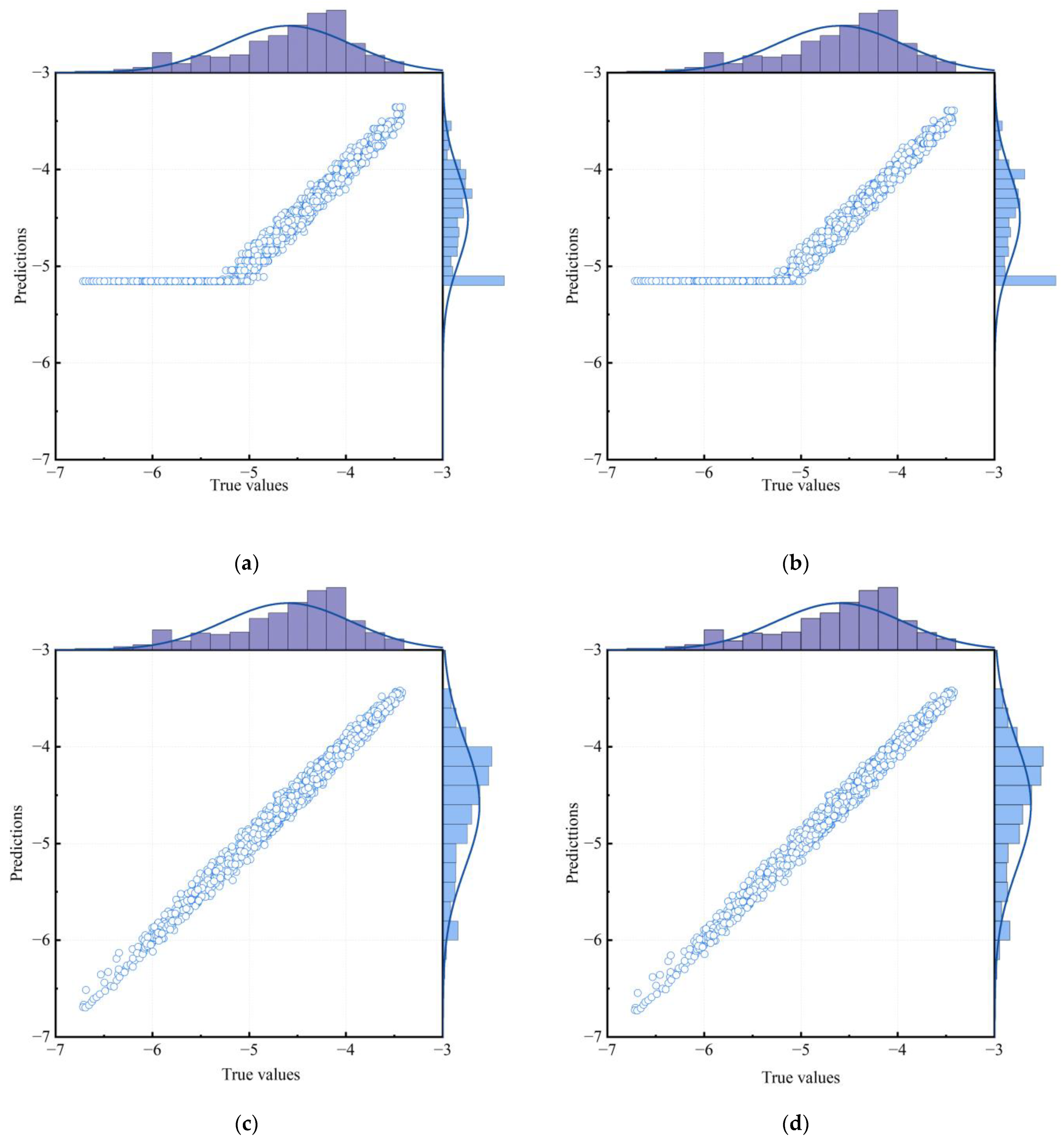
Marginal Histogram were developed by combining the predicted values from the model test set with the optimal parameters of the four models to further observe the performance of the models in predicting the vertical deformation of the wind turbine foundations, as shown in Figure 14. The middle section is a scatter plot of the true and predicted values, and the edge section is a histogram of the distribution of the true and predicted values and a normal distribution curve.

As can be seen from the tables and graphs, the DT and XGB models are the worst at predicting deformations, with a coefficient of determination of 0.810 on the test set. When the value of deformation is large, the predictions of both the DT model and the XGB model reach a critical phenomenon. This is due to the fact that both the XGB model and the DT model are essentially tree models, and when there is a certain range of data in the test set that is not involved in the training process, the unknown data enter the tree model to predict the clustering of the results, and the model will experience serious overfitting problems [38]. In addition, it can be learnt from the table and figure that the SVR model and LSTM model fit the data in the test set very well, and the coefficient of determination is as high as 0.992, which is the best prediction effect among all models.

As mentioned before, among all the developed models, the SVR model with hyperparameters C = 1, epsilon = 0.001, gamma = 0.01, and the LSTM model with hyperparameters activation = tanh, hidden_size = 128, epochs = 256 exhibit the best performance, efficiently predicting wind turbine settlement data with the highest R² value and the lowest MAE and MSE values.

While R² and other statistical measures can provide an overall picture of the performance of the model being developed, they do not provide information about the distribution and extent of errors. To compare more specifically the performance of the four models in predicting wind turbine foundation deformation, probability density distributions and function plots were plotted using Equation (15), as shown in Figure 15. Figure 15a shows the probability density distribution plots of the four machine learning models, showing the centralized distribution of the predicted/true values of the models, and Figure 15b shows the probability density cumulative plots of the four machine learning models, showing the cumulative probability share of the predicted/true values of the models.

$${\mathrm{f}}_h(x)=\frac{1}{nh}{\displaystyle \sum _{i=1}^{n}K(\frac{x-x_i}{h})}$$

(15)

where $k$ represents the kernel, $h$ is the smoothing parameter, and $n$ represents the number of sample data points.

As shown in Figure 15, the ratios of predicted values to actual values for the four models are distributed between 0.85 and 1.05. Among them, the SVR and LSTM models are the most stable, reaching a maximum value at a ratio of 1.0, which is higher than the other two models. On the other hand, the mean and standard deviation of the ratio between the predicted values and the actual values for the SVR model are 0.9991 and 0.0127. For the LSTM model, they are 1.0006 and 0.0128. These two models have the best prediction effect on foundation settlement. Moreover, it can be found from Figure 15a that the peak of the SVR model is concentrated at 1.0, implying that the predicted values are closer to the real values. In order to further observe the adaptability of the SVR and LSTM models in predicting the settlement of wind turbines foundation, the data of measuring points P-3, P-4 and P-5 were imported into the above two models for verification, and the prediction results are shown in

Table 6. Results from measurement points P-3, P-4, and P-5.

		R2	MSE × 10−3	MAE × 10−2
P-3	SVR	0.993	3.580	4.468
	LSTM	0.993	3.581	4.517
P-4	SVR	0.992	3.534	4.382
	LSTM	0.990	3.720	4.608
P-5	SVR	0.994	3.530	4.470
	LSTM	0.993	3.940	4.729

.

From the data in the table, it can be seen that the MAE and MSE values predicted by the SVR model for P-3, P-4, and P-5 measuring points are smaller than those predicted by the LSTM model, and the R² values predicted by the P-4 and P-5 measuring points are higher than those predicted by the LSTM model. This indicates that the comprehensive prediction performance of the SVR model is better than that of the LSTM model for all measurement points. The SVR model has stronger applicability in predicting wind turbine foundation deformation. The prediction performance of the SVR model for other measurement points is shown in Figure 16.

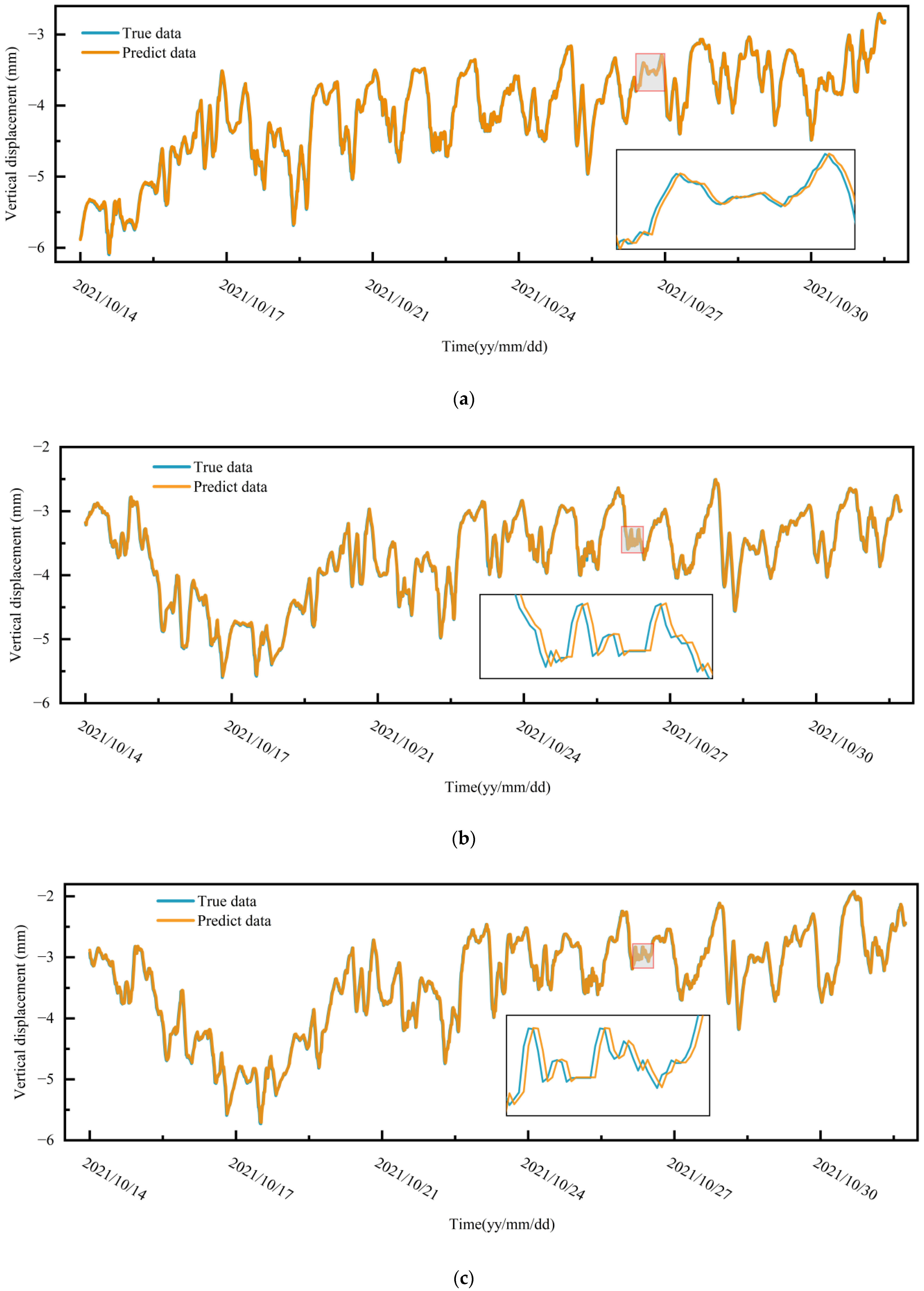
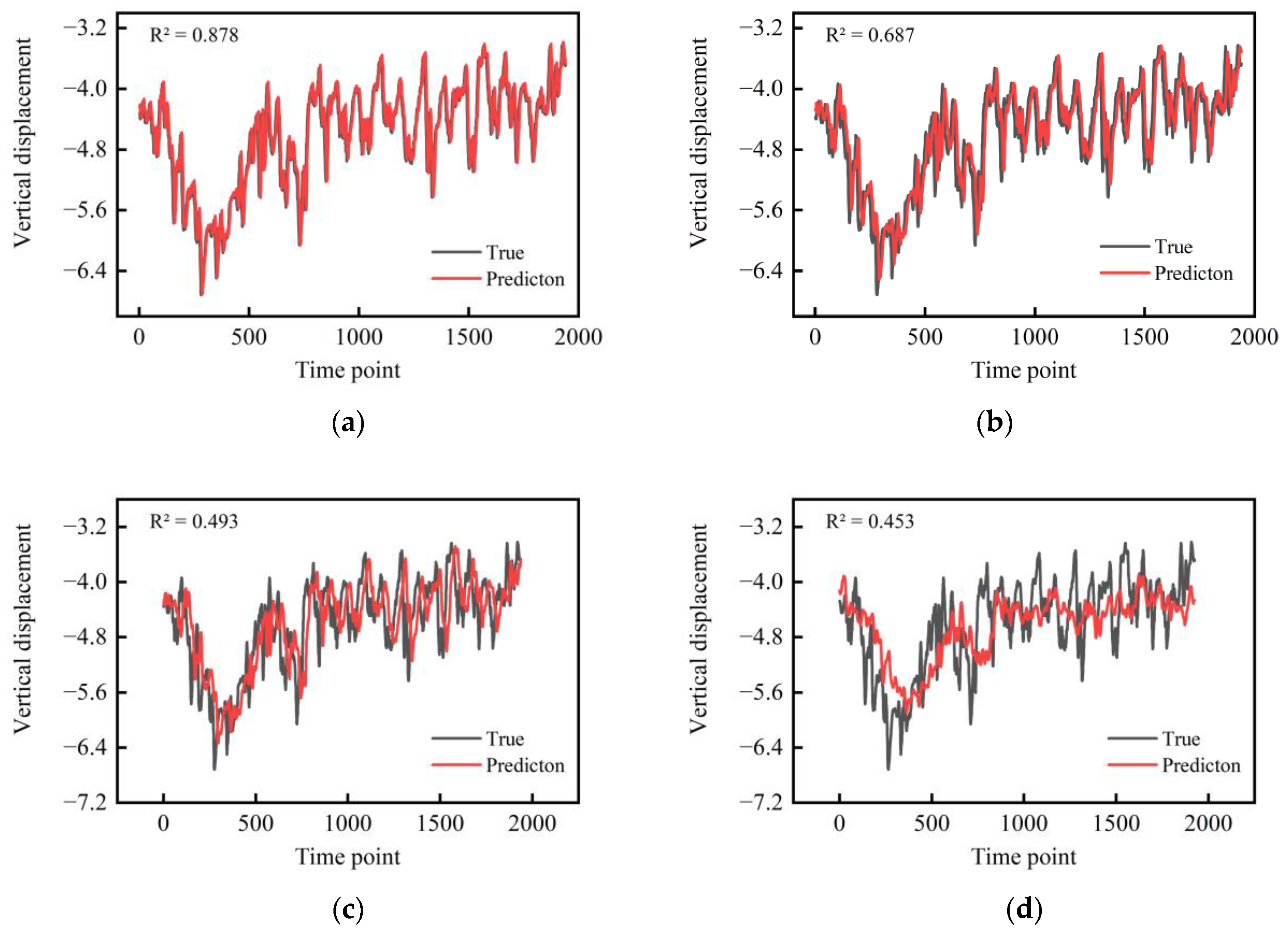
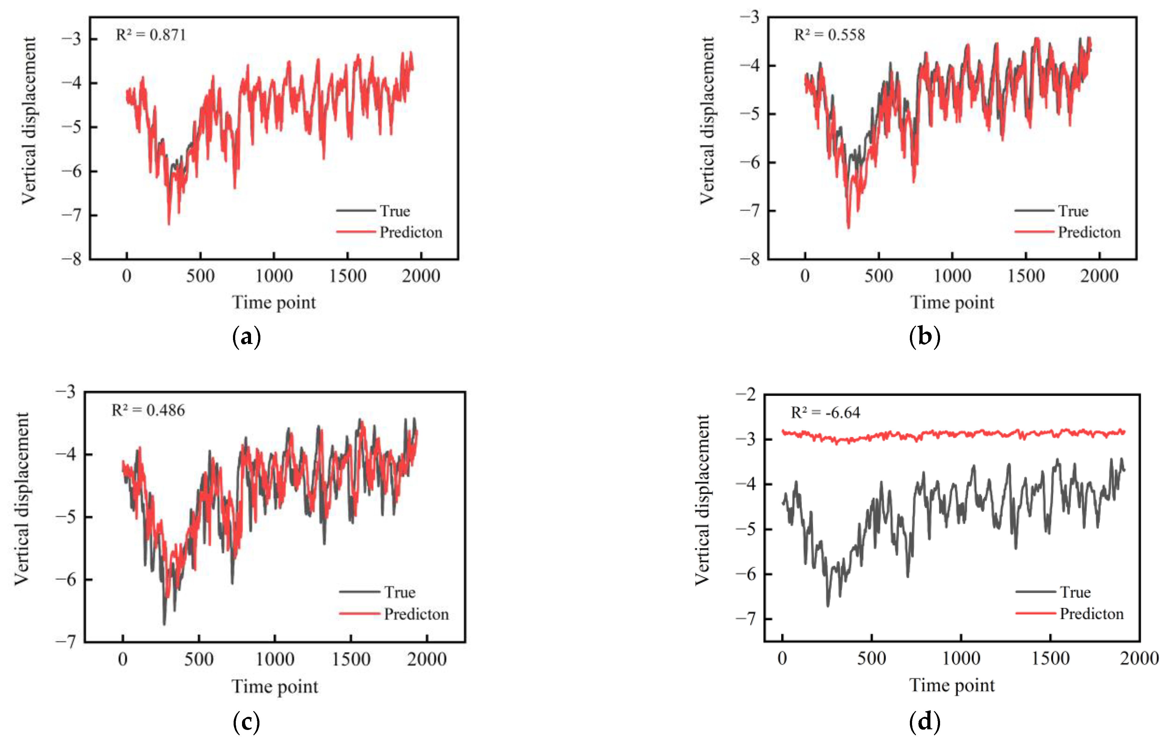
On this basis, we discuss the prediction of the measured points of the wind turbine foundation using the better-performing LSTM model and the SVR model, and here, the two models are used to quantitatively compare the multi-time-step prediction of the vertical displacement of the wind turbine foundation. The 5-time-step, 10-time-step, 20-time-step, and 50-time-step prediction tests are performed on the vertical displacement data of the wind turbine foundation. The performance of the two models for the prediction of wind turbine foundation displacement is further identified by comparing the multi-time-step prediction results.

The multi-time-step test results of the SVR model and LSTM model for the prediction of vertical displacement of wind turbine foundation are shown in Figure 17 and Figure 18, respectively. Firstly, comparing the two models with the same prediction step length, it can be found that both the SVR model and LSTM model perform well in the prediction of 5-time-step length, and at the same time, the R² value can reach 0.87, which indicates that the two models are more effective in the prediction of shorter time-step lengths. Secondly, in 10-time-step prediction, the LSTM model is slightly less effective than the SVR model, with a significant deviation in peak prediction around 300 Time point, which is less effective. In terms of 20-time-step prediction, both models perform poorly, with R² = 0.5 or less, and fail to achieve effective prediction of the base deformation. Finally, by comparing the 50-time-step prediction, it can be clearly found that the LSTM model has deviated from learning and predicting the base deformation law of the wind turbine, and the prediction of SVR can still fluctuate within the real interval in comparison, but the effect is still poor. The prediction effect of the model decreases significantly after 10 time steps, and the prediction effect of the subsequent 20 time steps and 50 time steps is poor. Such a phenomenon is due to the fact that the model only learns the short-term change characteristics of the wind turbine vertical displacement deformation during training, which yields a more accurate prediction for the next moment and shorter moments, however, it is difficult to get a long-term accurate prediction in the face of data spanning a large period of time. Multi-step prediction is still an open challenge in time series prediction [39].

Then, by comparing the experimental results of the SVR model with different step sizes, it can be found that the SVR model can still effectively learn and predict the displacement of the wind turbine foundation when it is predicted with shorter time steps (5 time steps and 10 time steps), but when the time step is increased to 20 time steps or 50 time steps when the time step is increased to 20 time steps or 50 time steps, the prediction effect is weakened and the accuracy decreases. By comparing the performance of the above models, it can be concluded that the SVR model and LSTM model have a higher short-time prediction accuracy and poorer long-time prediction effect in terms of wind turbine foundation displacement, while the SVR model is more advantageous in terms of learning the wind turbine foundation displacement data, its prediction effect and prediction accuracy are better than that of the LSTM model, and the trend prediction is closer to that of the LSTM model. The SVR model can be used to predict the future changes of the foundation of wind turbines so as to achieve the goal of predicting the future changes of the foundation of wind turbines. The SVR model can be utilized to predict future changes in wind turbine foundations, facilitating the assessment of the foundation’s future state after rehabilitation. However, the prediction of long-term changes in the base of wind turbines needs further study.

5. Conclusions

In a rehabilitation project for mountainous onshore wind turbine foundations, four machine learning models were developed and compared to analyze their effectiveness in predicting vertical deformation of wind turbine foundations. Various evaluation criteria were employed to assess the accuracy of different machine learning models. The reliability of the best model was confirmed by comparative analysis of field measurements. Based on the findings of this study, the following conclusions were made:

(1)

Following the rehabilitation of the foundation, during a specific time frame, the foundation deformation demonstrates conspicuous fluctuations due to the impact of external cyclic loads. However, over time, the overall deformation gradually reaches a state of stabilization.

(2)

Four machine learning models were developed to predict wind turbine foundation deformation. The SVR and LSTM models demonstrated the best performance among the developed models. The SVR model consistently achieved a coefficient of determination greater than 0.99 in the deformation prediction of the other three points and outperformed the LSTM model. This suggests that the overall applicability of the SVR model for predicting wind turbine foundation deformation is superior to that of the LSTM model.

(3)

In the comparison of the prediction multiple time steps, it can be clearly seen that the SVR model learns the wind turbine foundation displacement more accurately, and shows a better effect and higher accuracy in the prediction of short time steps. It can be seen that the SVR model is suitable for predicting the deformation of wind turbine foundations after repair, and can provide a reliable prediction of the subsequent wind turbine foundation deformation in order to assess the repair effect.

Obviously, the long-term prediction of vertical displacement deformation of wind turbine foundations shows a rather lower accuracy with the measured deformation development of wind turbine foundation. Based on this significant problem, the deep learning models would be modified based on some methods to enhance the long-term prediction of the deformation development of rehabilitated wind turbine foundation in future research.

References

1. Yao, G.; Yang, H.M.; Zhou, L.D.; Li, D.D.; Li, C.B.; Wang, J. Development status and key technologies of large-capacity offshore wind turbines. Autom. Electr. Power Syst. 2021, 45, 33–47. (In Chinese) [Google Scholar] [CrossRef]
2. Lu, W.R.; He, X.K.; Lu, B.R.; Shi, W.H.; Zhang, J.Z.; Zhu, F.; Zhu, M.Q. Fatigue damage mechanism of wind turbine foundation with foundation pipe. Build. Struct. 2018, 39, 140–148. (In Chinese) [Google Scholar] [CrossRef]
3. Janeliukstis, R. Continuous wavelet transform-based method for enhancing estimation of wind turbine blade natural frequencies and damping for machine learning purposes. Measurement 2020, 172, 108897. [Google Scholar] [CrossRef]
4. Kang, M.H.; Xu, H.; Hang, X. Local damage analysis of near foundation ring in wind turbine foundation. Acta Energiae Solaris Sin. 2014, 35, 583–588. (In Chinese) [Google Scholar]
5. Guo, Y.; Zhang, P.; Ding, H.; Le, C. Experimental Study on Torsion Resistance of Foundation Ring Land-Based Wind Power Expanded Foundation Scale Model. Appl. Sci. 2020, 10, 5612. [Google Scholar] [CrossRef]
6. Velarde, J.; Kramhøft, C.; Sørensen, J.D. Global sensitivity analysis of offshore wind turbine foundation fatigue loads. Renew. Energy 2019, 140, 177–189. [Google Scholar] [CrossRef]
7. Amponsah, E.; Wang, Z.; Mantey, S.K. Bending-bearing behaviour of embedded steel ring-foundation connection of onshore wind turbines. Structures 2021, 34, 180–197. [Google Scholar] [CrossRef]
8. McAlorum, J.; Perry, M.; Fusiek, G.; Niewczas, P.; McKeeman, I.; Rubert, T. Deterioration of cracks in onshore wind turbine foundations. Eng. Struct. 2018, 167, 121–131. [Google Scholar] [CrossRef]
9. Sun, L.Y.; Huang, H.; Zhen, L.; Xia, S.F. Optimization design of foundation reinforcement scheme for low strength wind turbine based on plastic damage model. Acta Energiae Solaris Sin. 2022, 43, 453–460. (In Chinese) [Google Scholar] [CrossRef]
10. Chen, J.; Chen, Y.; Mao, B.; Wang, X.; Peng, L. Key mitigation regions and strategies for CO2 emission reduction in China based on STIRPAT and ARIMA models. Environ. Sci. Pollut. Res. 2022, 29, 51537–51553. [Google Scholar] [CrossRef]
11. Mohamed, W.; Austrell, P.E. A comparative study of three onshore wind turbine foundation solutions. Comput. Geotech. 2017, 94, 46–57. [Google Scholar] [CrossRef]
12. Tang, Q.; Dang, J.; Cui, Y.; Wang, X.; Jia, J. Machine learning-based fast seismic risk assessment of building structures. J. Earthq. Eng. 2022, 26, 8041–8062. [Google Scholar] [CrossRef]
13. Wong, P.T.; Lai, W.W. Harmonising Cross-System GPR Wave Amplitude for Concrete Diagnosis with Machine Learning. J. Nondestruct. Eval. 2023, 42, 99. [Google Scholar] [CrossRef]
14. Liu, M.; Liao, S.; Yang, Y.; Men, Y.; He, J.; Huang, Y. Tunnel boring machine vibration-based deep learning for the ground identification of working faces. J. Rock Mech. Geotech. Eng. 2021, 13, 1340–1357. [Google Scholar] [CrossRef]
15. Wu, B.; Wan, Y.; Xu, S.; Zhao, C.; Liu, Y.; Zhang, K. A Multi-Source Intelligent Fusion Assessment Method for Dynamic Construction Risk of Subway Deep Foundation Pit: A Case Study. Sustainability 2023, 15, 10162. [Google Scholar] [CrossRef]
16. Samui, P. Support vector machine applied to settlement of shallow foundations on cohesionless soils. Comput. Geotech. 2008, 35, 419–427. [Google Scholar] [CrossRef]
17. Kirts, S.; Nam, B.H.; Panagopoulos, O.P.; Xanthopoulos, P. Settlement prediction using support vector machine (SVM)-based compressibility models: A case study. Int. J. Civ. Eng. 2019, 17, 1547–1557. [Google Scholar] [CrossRef]
18. Raja, M.N.; Shukla, S.K. Multivariate adaptive regression splines model for reinforced soil foundations. Geosynth. Int. 2021, 28, 368–390. [Google Scholar] [CrossRef]
19. Deng, J.; Zeng, T.; Yuan, S.; Fan, H.; Xiang, W. Interval Prediction of Building Foundation Settlement Using Kernel Extreme Learning Machine. Front. Earth Sci. 2022, 10, 939772. [Google Scholar] [CrossRef]
20. Pourtaghi, A.; Lotfollahi-Yaghin, M.A. Wavenet ability assessment in comparison to ANN for predicting the maximum surface settlement caused by tunneling. Tunn. Undergr. Space Technol. 2012, 28, 257–271. [Google Scholar] [CrossRef]
21. Vidal, Y.; Aquino, G.; Pozo, F.; Gutiérrez-Arias, J.E. Structural health monitoring for jacket-type offshore wind turbines: Experimental proof of concept. Sensors 2020, 20, 1835. [Google Scholar] [CrossRef] [PubMed]
22. Leon-Medina, J.X.; Parés, N.; Anaya, M.; Tibaduiza, D.A.; Pozo, F. Ensemble of feature extraction methods to improve the structural damage classification in a wind turbine foundation. Bull. Pol. Acad. Sci. Tech. Sci. 2023, 71, 144606. [Google Scholar] [CrossRef]
23. Jiang, S.; Mao, H.; Ding, Z.; Fu, Y. Deep Decision Tree Transfer Boosting. IEEE Trans. Neural Netw. Learn. Syst. 2019, 31, 383–395. [Google Scholar] [CrossRef] [PubMed]
24. Shorabeh, S.N.; Samany, N.N.; Minaei, F.; Firozjaei, H.K.; Homaee, M.; Boloorani, A.D. A decision model based on decision tree and particle swarm optimization algorithms to identify optimal locations for solar power plants construction in Iran. Renew. Energy 2022, 187, 56–67. [Google Scholar] [CrossRef]
25. Chen, T.; Guestrin, C. Xgboost: A scalable tree boosting system. In Proceedings of the 22nd ACM SIGKDD International Conference on Knowledge Discovery and Data Mining, San Francisco, CA, USA, 13–17 August 2016; pp. 785–794. [Google Scholar] [CrossRef]
26. Purohit, S.; Ng, E.Y.K.; Kabir, I.F.S.A. Evaluation of three potential machine learning algorithms for predicting the velocity and turbulence intensity of a wind turbine wake. Renew. Energy 2022, 184, 405–420. [Google Scholar] [CrossRef]
27. Jahangiri, B.; Barri, K.; Alavi, A.H.; Buttlar, W.G. A molecular sensing method integrated with support vector machines to characterize asphalt mixtures. Measurement 2021, 179, 109528. [Google Scholar] [CrossRef]
28. Sun, Y.; Ding, S.; Zhang, Z.; Jia, W. An improved grid search algorithm to optimize SVR for prediction. Soft Comput. 2021, 25, 5633–5644. [Google Scholar] [CrossRef]
29. Liu, H.; Mi, X.; Li, Y.; Duan, Z.; Xu, Y. Smart wind speed deep learning based multi-step forecasting model using singular spectrum analysis, convolutional Gated Recurrent Unit network and Support Vector Regression. Renew. Energy 2019, 143, 842–854. [Google Scholar] [CrossRef]
30. Belagoune, S.; Bali, N.; Bakdi, A. Deep Learning through LSTM Classification and Regression for Transmission Line Fault Detection, Diagnosis and Location in Large-Scale Multi-Machine Power Systems. Measurement 2021, 177, 109330. [Google Scholar] [CrossRef]
31. Ding, Y.; Zhu, Y.; Feng, J.; Zhang, P.; Cheng, Z. Interpretable spatio-temporal attention LSTM model for flood forecasting. Neurocomputing 2020, 403, 348–359. [Google Scholar] [CrossRef]
32. López, G.; Arboleya, P. Short-term wind speed forecasting over complex terrain using linear regression models and multivariable LSTM and NARX networks in the Andes Mountains, Ecuador. Renew. Energy 2022, 183, 351–368. [Google Scholar] [CrossRef]
33. Lee, D.H.; Cheon, E.; Lim, H.H.; Choi, S.K.; Kim, Y.T.; Lee, S.R. An artificial neural network model to predict debris-flow volumes caused by extreme rainfall in the central region of South Korea. Eng. Geol. 2021, 281, 105979. [Google Scholar] [CrossRef]
34. Olu-Ajayi, R.; Alaka, H.; Sulaimon, I.; Sunmola, F.; Ajayi, S. Building energy consumption prediction for residential buildings using deep learning and other machine learning techniques. J. Build. Eng. 2022, 45, 103406. [Google Scholar] [CrossRef]
35. El-Mir, A.; El-Zahab, S.; Sbartaï, Z.M.; Homsi, F.; Saliba, J.; El-Hassan, H. Machine learning prediction of concrete compressive strength using rebound hammer test. J. Build. Eng. 2023, 64, 105538. [Google Scholar] [CrossRef]
36. Hwang, S.H.; Mangalathu, S.; Shin, J.; Jeon, J.S. Machine learning-based approaches for seismic demand and collapse of ductile reinforced concrete building frames. J. Build. Eng. 2021, 34, 101905. [Google Scholar] [CrossRef]
37. Dong, X.C.; Gou, M.W.; Wang, S.L. Prediction of sinking rate of sinkhole foundation based on multivariate structural stress characteristics. J. Rock Mech. Eng. 2022, 41 (Suppl. S2), 3476–3487. (In Chinese) [Google Scholar] [CrossRef]
38. Hasan, M.R.; Siraj, F.; Sainin, M.S. Improving ensemble decision tree performance using Adaboost and Bagging. In Proceedings of the 2nd Innovation and Analytics Conference and Exhibition, Kedah, Malaysia, 29 September–1 October 2015. [Google Scholar] [CrossRef]
39. Taieb, S.B.; Bontempi, G.; Atiya, A.F.; Sorjamaa, A. A review and comparison of strategies for multi-step ahead time series forecasting based on the NN5 forecasting competition. Expert Syst. Appl. 2012, 39, 7067–7083. [Google Scholar] [CrossRef]
Figure 1. The site location of #22 wind turbine.
Buildings 14 00759 g001
Figure 2. Wind turbine foundation structure and strata section.
Buildings 14 00759 g002
Figure 3. Cracks in wind turbine foundations.
Buildings 14 00759 g003
Figure 4. Rehabilitation project for the wind turbine foundation.
Buildings 14 00759 g004
Figure 5. Installation position of the static level on the wind turbine foundation.
Buildings 14 00759 g005
Figure 6. Installation of the reference point of the static level.
Buildings 14 00759 g006
Figure 7. Comparative curves of wind speed at the site, turbine rotational speed, and vertical displacement of the wind turbine foundation.
Buildings 14 00759 g007
Figure 8. The overall process of the model building.
Buildings 14 00759 g008
Figure 9. Simplified structure of the Decision Tree model.
Buildings 14 00759 g009
Figure 10. Mechanisms of the Support Vector Regression (SVR) model.
Buildings 14 00759 g010
Figure 11. Long Short-Term Memory (LSTM) model cell.
Buildings 14 00759 g011
Figure 12. Comparison of data before and after filtering.
Buildings 14 00759 g012
Figure 13. Evaluating and selecting the parameters of the model.
Buildings 14 00759 g013
Figure 14. Marginal histogram of results plotted for the four models: (a) DT model; (b) XGB model; (c) SVR model; and (d) LSTM model.
Buildings 14 00759 g014
Figure 15. Probability correlation curves based on the model results: (a) density chart, (b) cumulative probability chart.
Buildings 14 00759 g015
Figure 16. Comparison of the predicted and actual results of the SVR model for various measurement points: (a) Point 3; (b) Point 4; and (c) Point 5.
Buildings 14 00759 g016
Figure 17. SVR model test: (a) 5 time steps; (b) 10 time steps; (c) 20 time steps; and (d) 50 time steps.
Buildings 14 00759 g017
Figure 18. LSTM model test: (a) 5 time steps; (b) 10 time steps; (c) 20 time steps; and (d) 50 time steps.
Buildings 14 00759 g018