Experimental Study of Wind Pressures on Low-Rise H-Shaped Buildings

Abstract

Recognizing the urgent need for mitigating global warming, natural ventilation presents a potential strategy to reduce cooling energy demands, enhance thermal comfort, and contribute to indoor air quality. H-shaped buildings are prevalent worldwide, and they constitute the majority of the social housing construction in Brazil. Research suggests that the inadequate design of these buildings can result in poor ventilation; however, investigations about their natural ventilation performance are limited. Thus, the present contribution aims to determine the impact of the geometric characteristics of H-shaped buildings on the pressure distribution through wind tunnel experiments. Three models were tested in the wind tunnel experiments, representing different proportions. Their scales were configured to comply with the 5% obstruction limit allowed for wind tunnel testing, which was performed for 20 wind attack angles. Moreover, a scour test was carried out to allow a better understanding of the wind flow. Python scripting was developed to automate data processing, which is openly available in this paper. The results indicate that the proportion of the model influences the pressure distribution on roofs and leeward walls. Additionally, the depth of the recessed cavity affects its side surfaces and can result in a mirrored behavior on the frontal face of deep cavities (i.e., the wind direction is 45°). The model height influences the windward surfaces in its lower portion, since taller models present a recirculation vortex that modifies the pressure near the ground.

1. Introduction

As the greenhouse gas concentration continues to grow in the atmosphere (currently 54% higher than in 1990), it is already causing climate changes and impacts on the environment [1]. A substantial decrease in energy consumption is recommended as one way to mitigate global warming [1]. In the built environment, natural ventilation is a passive strategy that has significant potential for reducing cooling energy demands and improving thermal comfort in hot climates [2,3]. In addition, it contributes to indoor air quality, thus reducing the risk of airborne disease transmission, such as COVID-19 [4,5].

The H-shaped floor plan is a relevant building topology. In addition to being a common design for residential [6,7] and commercial [8] buildings, it is the most common social housing typology for multifamily buildings in Brazil [9], which are typically constructed in suburban areas, where most buildings are low-rise buildings [9]. Moreover, it is noteworthy that Brazil has been heavily investing in social housing, having financed 3,828,054 residential units through the funding program “Minha Casa Minha Vida” between 2009 and 2020 [10]. This underscores the impact that well-designed natural ventilation systems, for this typology, can have on the thermal comfort and quality of life of thousands of Brazilians. This design is of interest to construction companies because it enables the good use of space and presents a larger perimeter than rectangular floor plans, allowing for more naturally ventilated rooms [11]. Nonetheless, a study conducted with two H-shaped buildings in Campinas, Brazil, revealed that at least fifty percent of the apartments were poorly ventilated due to the placement of the windows and the solar orientation of the building, not following the recommendations for thermal comfort [12]. Additionally, a worrying fact is that in tall buildings, when the wind is perpendicular to the cavities, the air can stagnate, becoming a threat to fire safety [13]. Moreover, this feature can cause severe health issues, as it was responsible for the deaths of hundreds of people in a severe acute respiratory syndrome (SARS) outbreak [14]. Thus, it is essential to understand the ventilation of H-shaped buildings to provide good ventilation systems by making proper use of their attributes.

Regarding ventilation studies, numerical simulations have recently become a popular method because of the computing power of current hardware. In the field of thermal comfort, Building Energy Simulations (BESs) are one of the most common choices. Furthermore, these BESs can be coupled with airflow network (AFN) models, allowing for the study of the effect of natural ventilation on energy consumption and thermal comfort in buildings [15]. Despite these benefits, to perform AFN simulations, building modelers need to input wind pressure coefficient (Cp) data for various wind incidences. The accuracy of these data is essential for obtaining reliable results [16]. The Cp is a dimensionless coefficient that represents the static pressure measured at a given point normalized by the reference pressure measured at the model’s height [17]; see Equation (2) for further details. These data can be used for research applications for high-rise [18,19] and low-rise buildings [20]. Cp data can be obtained by performing wind tunnel tests [21] and computational fluid dynamics (CFDs) simulations [22], and by searching databases [23]. The easiest approach is to obtain Cp data from an existing database or a case study equivalent to the target model. However, although several Cp databases and publications on this subject are available, they are mostly for buildings with rectangular floor plans [17].

Concerning shapes with recessed bays, a few studies have investigated wind pressure behavior in H and C-shaped buildings, especially for high-rise buildings. In general, studies show that the recessed cavities of both of these building shapes have a low average influence on wind-induced loads and dynamic responses [6,24] and could even be considered negligible [24]. However, in a detailed analysis, it was found that, at normal wind incidence, the leeward cavities of H-shaped buildings have reduced crosswind excitation compared to rectangular ones [6]. This phenomenon can be related to pumping ventilation [25,26,27] and to building vortex shedding [28]. Overall, the use of averaged values masks the nuances in the results, and detailed analyses are needed for complex building shapes.

Regarding air quality in C-shaped buildings, it was observed that depending on the location of the pollutant emission source, C-shaped buildings showed different levels of effectiveness [29,30]. When pollution comes from the roof, their performance was better than in the case of a rectangular plan (with the C floor plan being recommended for better air quality). However, with pollutants originating from the central courtyard or near the rear face of the cavity, ventilation was worse than the rectangular building in terms of gas dilution [29,30].

Also, both H-shaped [13] and C-shaped [31,32] buildings exhibit low air velocities in the cavity region, especially if they are located in the wake region (parallel to the wind direction or leeward), since ventilation is indirect and occurs by suction. Researchers also found that, for 0° wind incidence, H-buildings with a wider cavity were better ventilated [31] and presented a wider pressure range; additionally, C-shaped buildings with deep recesses presented lower wind pressure values on leeward surfaces [33]. As well, for a wind attack of 90°, in H-shaped models the depth was the parameter that most influenced ventilation (shallow reentrances were recommended to improve air quality) [31]. Furthermore, taller buildings of the same archetype presented lower ventilation rates in the cavity region [13].

Considering the influence of adjacent building shapes on drag forces, tall H-shaped buildings created higher airflow resistance in the neighboring block compared to the square floor plan, leading to a reduction in the average Cp by up to 50% [34]. In a group of low-rise buildings, this form also showed high wind resistance, reducing the ventilation that reached the rear rows [20]. In addition, these authors observed a lower potential for cross-ventilation in openings located in the cavities (i.e., at windward and leeward directions) compared to the same area in a rectangular floor plan.

It is hypothesized that the cavity in a tall building could proportionally be considered a narrow recess, reducing the shape effect on wind flow. Otherwise, low-rise buildings (with a height/width ratio lower than 4 [35]) may be more susceptible to the influence of wind-induced ventilation due to their scale, which is worth exploring.

Therefore, the aim of this research is to study the surface pressure distribution of three H-shaped low-rise models by performing wind tunnel tests, seeking to comprehend the influence of this building’s shape parameters (height, proportions, and depth of the recessed cavity) on the pressure distribution behavior. For this, the wind tunnel flow was configured as a suburban atmospheric boundary layer (ABL) using mixed roughness elements and Couhinan vortex generators, and then the models were tested in 20 wind directions. In addition, scour tests were conducted to visualize the wind flow around the models at ground level.

The paper is structured as follows: after this introduction, Section 2 presents the building models, wind tunnel facilities, measurement systems, and data-processing tools. The results and discussion are given in Section 3, while Section 4 is devoted to the conclusions.

2. Materials and Methods

This section introduces the main experimental setup. The work method has been organized into four steps: (i) the definition of the model’s dimensions, materials, and location of pressure taps; (ii) the production and assembly of the model, as well as the installation of the pressure measurement system; (iii) the wind tunnel configuration to represent the desired atmospheric boundary layer, followed by the tests; and (iv) data processing, allowing for the analysis of the results.

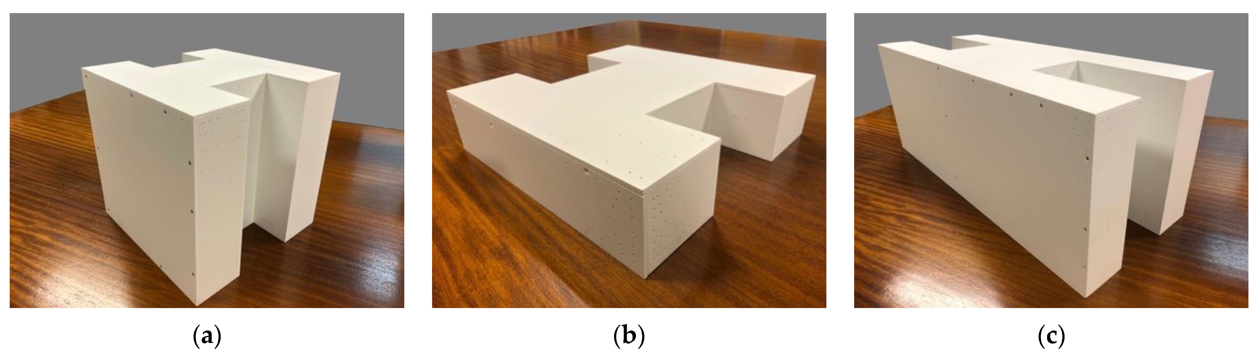
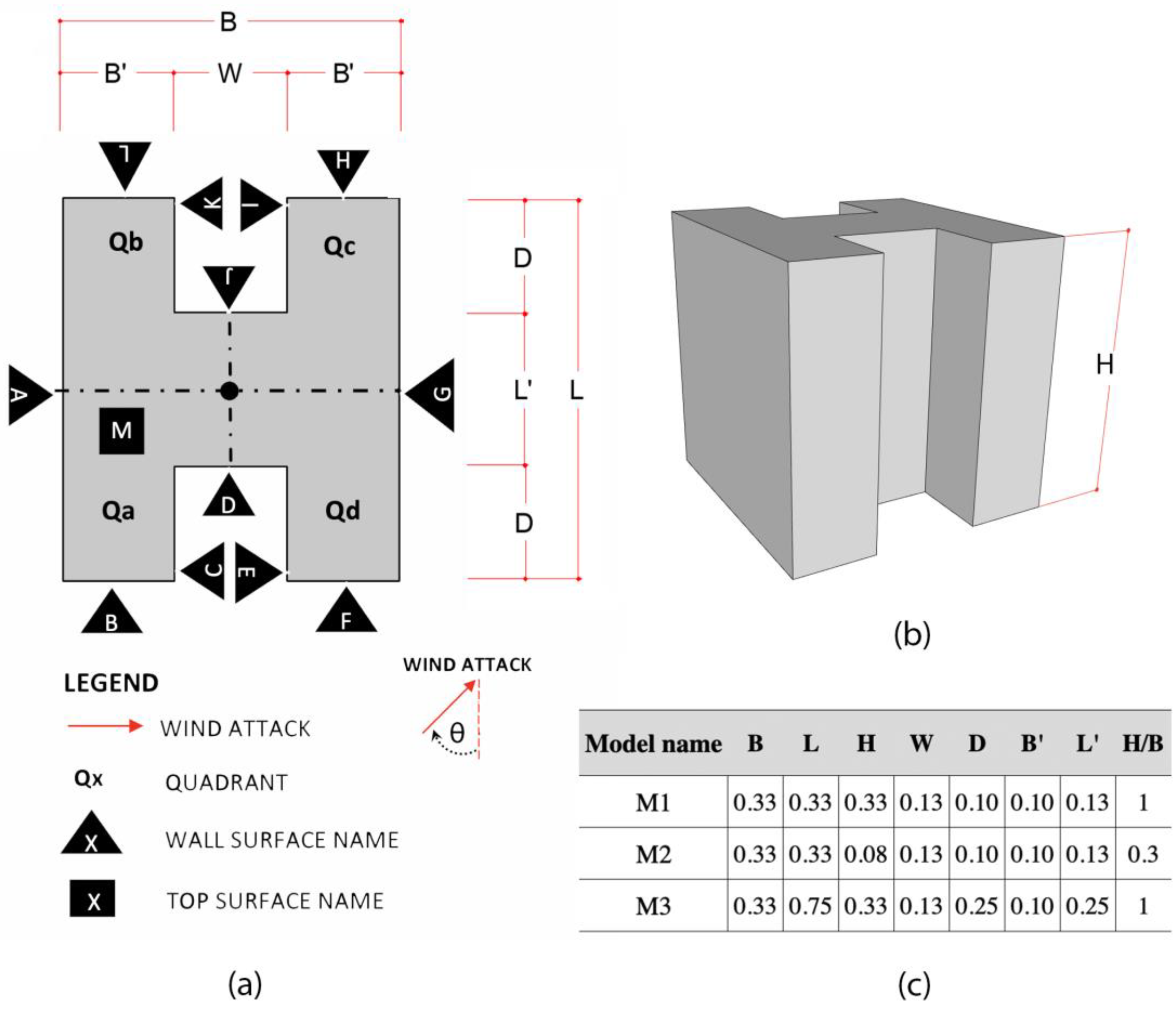
2.1. Building Models

The physical models were constructed using 4 mm PVC, ensuring model stability. Figure 1 shows pictures of the three models, showing the difference in height and proportion between them. The first model (M1—Figure 1a) has unitary aspect ratios, the proportions of the second one (M2—Figure 1b) represent horizontally designed structures such as hospital or school facilities, while the dimensions of the third one (M3—Figure 1c) maximize the reentrant bay.

The geometry characterization of the models can be found in Figure 2a (floor plan) and Figure 2b (model perspective), where the following parameters are described: the breadth (B), length (L), and height (H) of the building, and the width (W) and depth (D) of the cavities. Additionally, the height-to-width (H/B) ratio is presented. To provide more space for the pressure sensors and enable the higher resolution of the results, it was decided to adopt the largest scale allowed; given the limit of 5% obstruction [36] and the working area of the wind tunnel (6 m²), the model was fitted to a scale of 1:60 and presented a maximum of 4.6% obstruction. The height-to-width (H/B) ratio of the models ranges from 1 to 0.3 (Figure 2c), configuring them as low-rise buildings [35]. Figure 2c shows the reduced model dimensions in meters.

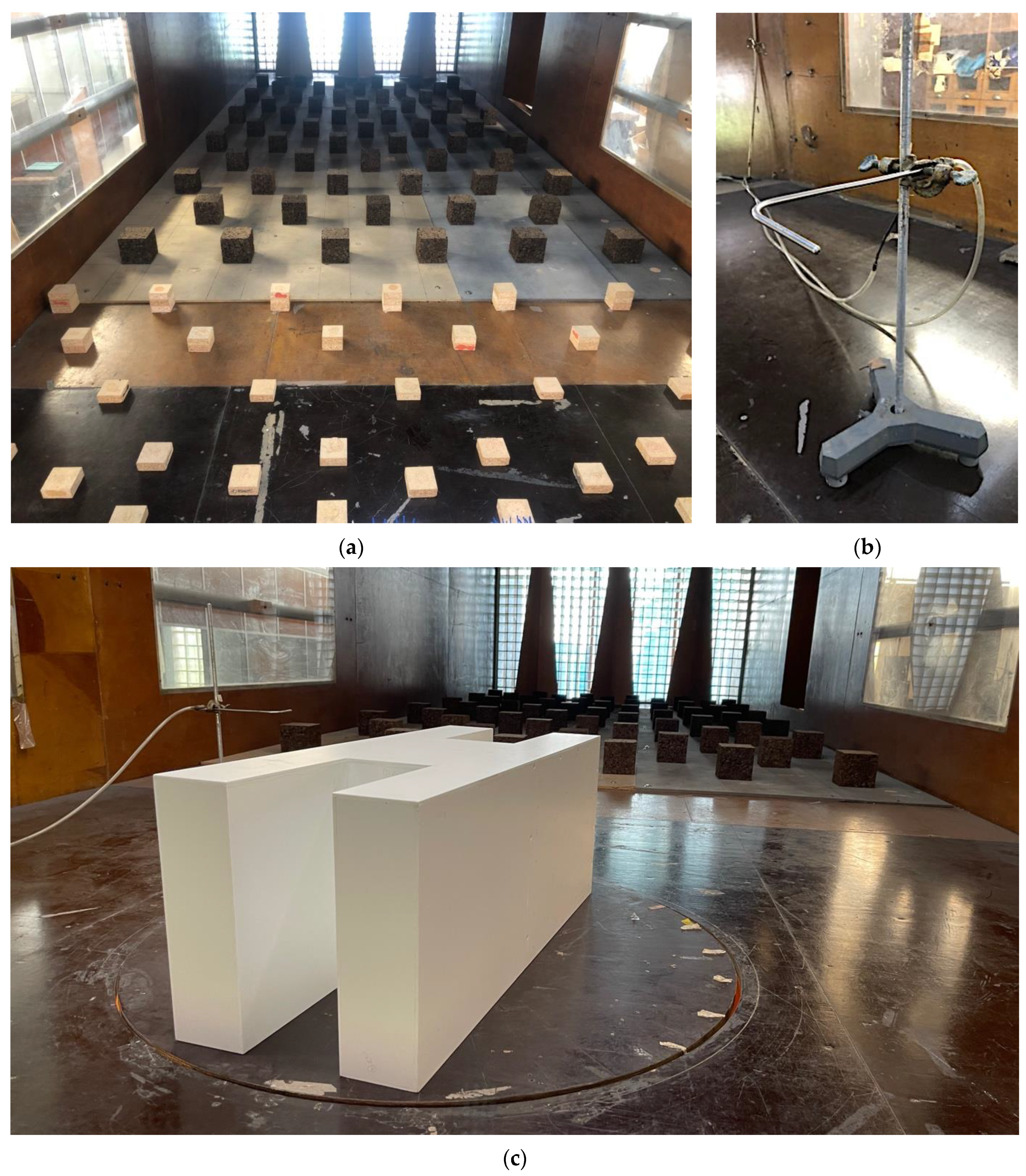
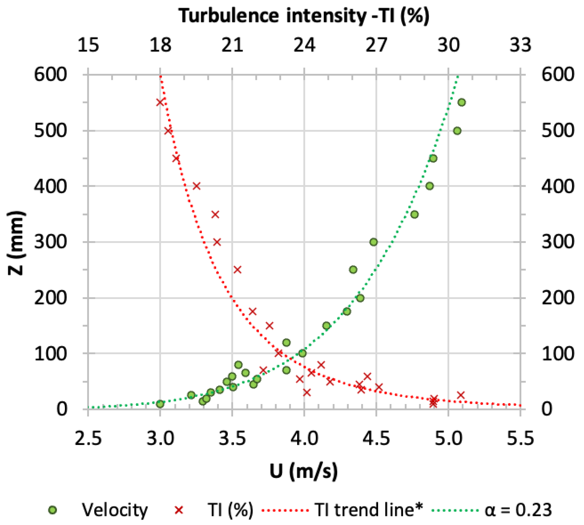
2.2. Experimental Setup

The tests were performed in an open-circuit wind tunnel located at the Structures Department in the National Laboratory of Civil Engineering (LNEC), in Lisbon, Portugal. The testing section is 9.0 m long, with a width of 3.1 m and a height of 2.0 m. A turntable allows for easily evaluating different wind incidences. In this regard, 20 wind attack angles (θ) were established as follows: 0°, 10°, 20°, 30°, 45°, 60°, 90°, 120°, 135°, 150°, 160°, 170°, 180°, 225°, 270°, 300°, 315°, 330°, 340°, and 350°, clockwise, as shown in Figure 2a. The angle step is not constant, as it was chosen based on the complexity of the expected flow behavior. Since the measurement points were placed in quadrant Qa, the angles close to the start or the end of the windward condition for Qa (0° and 180°) have a smaller angle step.

A suburban ABL [37] was chosen to properly represent the surrounding conditions of the buildings. This wind profile has been adopted in similar studies [38,39]. The ABL wind profile used in our experiments provides a generic characterization for such suburban areas; although it requires isolation to maintain generality, it represents the typical situation of the research object. Then, to reproduce the ABL as closely as possible, triangular spires and cubic staggered roughness elements were placed in the first section of the wind tunnel, as shown in Figure A2 (see Appendix A for further details, including photos).

Figure 3 shows the turbulence intensity and velocity conditions in the wind tunnel. The velocity profile was measured in an empty wind tunnel (without the building model) using a pitot tube positioned at the turntable’s center. It was then adjusted to the desired height for each sample. The nondimensional coefficient (α = 0.23) and the reference velocity U_s (4 m/s) at a given height Z_s (0.2 m) were determined by fitting a power law velocity profile [16], which is defined as follows:

U = U_s (Z/Z_s)^α

(1)

where U [m/s] is the wind speed at height Z [m] at a certain point; U_s [m/s] is the wind speed at height Z_s [m], which is the reference height; and α is the nondimensional power-law coefficient. The minimum Re is 2.4 × 10⁴, taking the models height as a reference dimension.

It is important to highlight that the pRef (test reference flow dynamic pressure) was measured at 70 cm to the side of the turntable’s center and at the models’ heights to avoid influencing the flow around the building models.

2.3. Measurements

Taking advantage of the model’s symmetries, pressure taps were distributed throughout the surfaces of a quarter of the models (Qa, Figure 2a). Additionally, a denser tap distribution was made close to the corners and edges. Furthermore, the number of tap points was limited by physical constraints due to the model scale. To achieve the desired tap distribution, the following number of tap points per model was used: 225 (M1), 175 (M2), and 262 (M3). The locations of the measurement taps are provided in [40] for further information see Supplementary Materials.

PSI^® DTC miniature ESP pressure scanners were used to obtain the pressure data from the wind tunnel tests (Figure A1b); the scanners were connected to a computer, and read by the software [41]. For every wind attack angle and to guarantee statistically converged pressure data, samples were acquired for approximately 200 s (2 Hz sampling frequency). Figure A1a (included in the Appendix A) shows an example of a model ready to be closed and undergo the wind tunnel test.

Additionally, a scour test was performed to obtain a visualization of the wind ground flow around the models, which is commonly performed in similar experiments [42]. First, a single layer of calibrated sand, small enough to be immersed in the ABL viscous layer (using an ASTM series sieve with 1–0.5 mm), was spread on the floor of the wind tunnel (around the model). Whenever drag exceeds shear, the sand particles move, allowing us to visualize the action of the wind at ground level.

2.4. Data Processing

The data processing was implemented in five steps, which were repeated for all three models and wind attack angles as follows:

I.

The dynamic pressure measured on the model surfaces was converted to Cp as follows:

Cp = (pRaw − pZero)/pRef,

(2)

where pRaw is the static pressure raw data obtained from the wind tunnel with residual noise, pZero is the (electric) noise pressure value measured with the fans turned off [43], and pRef is the reference flow dynamic pressure measured at 70 cm to the side of the turntable’s center at the models’ heights.

II.

Then, considering that only the first quadrant (Qa) of the model was equipped, the next step was to mirror the data to the rest of the model (quadrant divisions can be found in Figure 2a). The formula used to obtain the respective angle for each quadrant can be found in the appendix (Equations (A1)–(A3)).

III.

Cp values were time-averaged and exported in the appropriate format to generate the surface Cp contours in SURFER 7^®.

IV.

The mentioned contour images were manually generated in Surfer 7^® [44].

V.

Next, the numeric data were organized and plotted in graphics, as presented in Section 3.

All steps in the data process, except step IV, were automated through a routine implemented in Python using the development environment Spyder 5.1.5 [45]. The routine calculates the Cp, organizes the data, locates possible sensor errors, and produces the following outputs: (i) CSV files that can be read by SURFER 7^®, and (ii) a “read me” file with information about the data treatment. In this manner, data processing is less prone to human error and much faster than manual manipulation. The code, user instructions, and examples are provided in [46] for further information see Supplementary Materials.

3. Results and Discussion

The main findings of the research are presented in this section. The results were analyzed in two scales of detail: first, the Cp values along the horizontal and vertical centerlines are compared; and finally, the Cp distribution (contours) is presented.

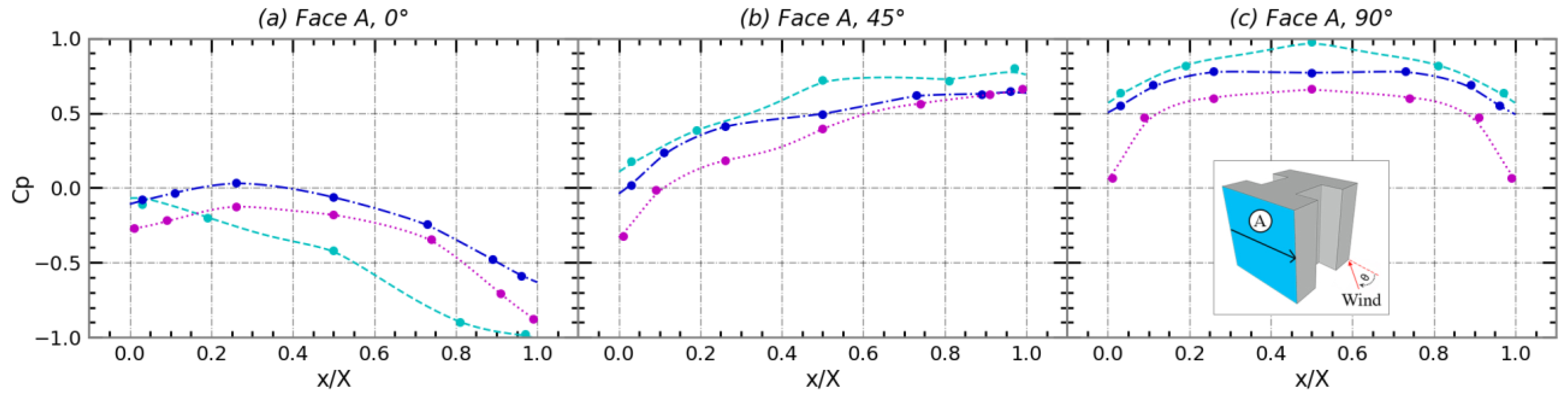
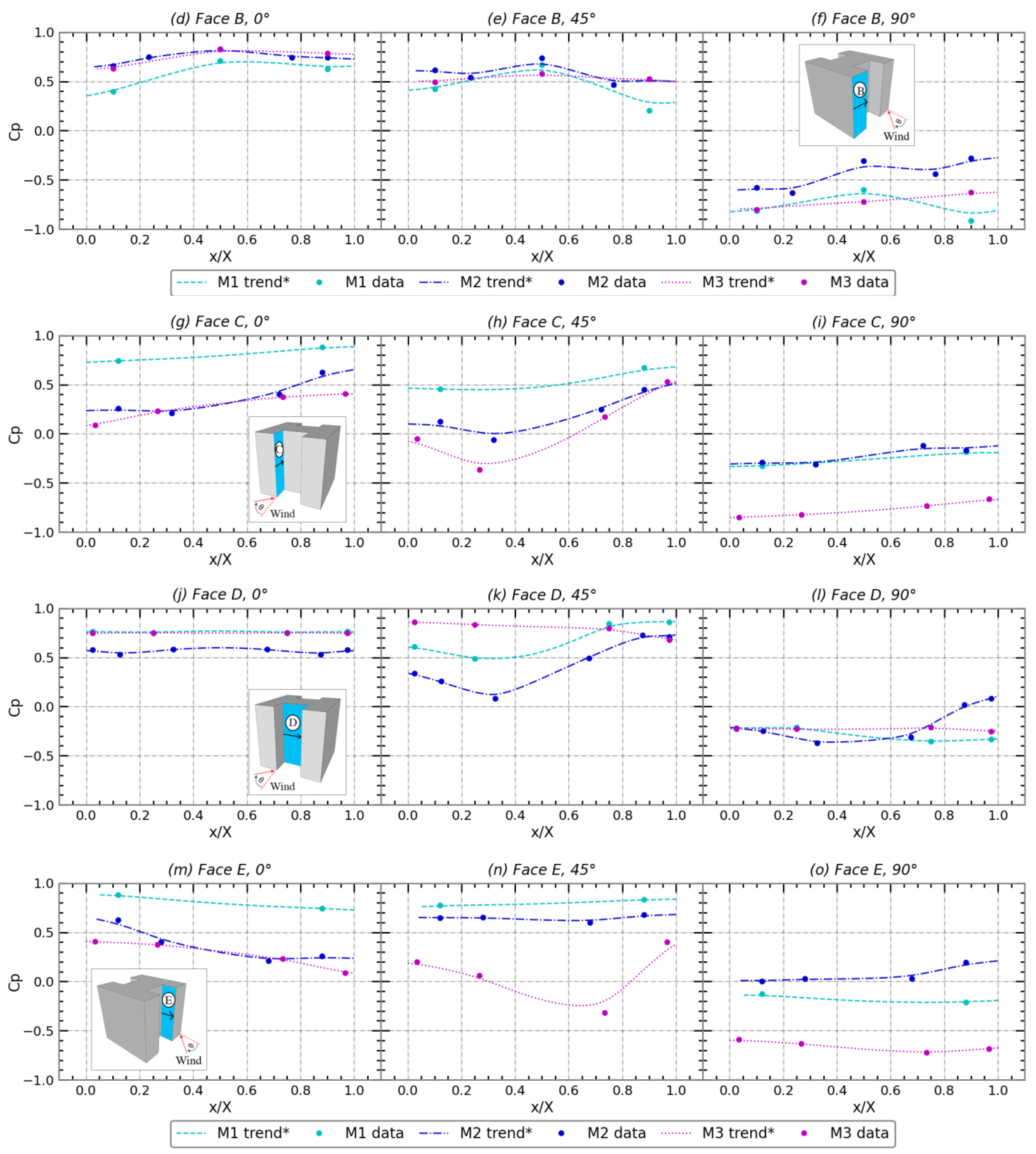
3.1. Horizontal Pressure Distribution

To understand the general influence of these buildings’ shapes on the wind pressure behavior, we compared the Cp values (at half-height and along the surfaces) between the models. To plot the data on a comparable scale, the horizontal component was made dimensionless by considering the ratio of the distance from the left edge to the measured point, x, and the surface total length, X. As shown in Figure 4, the zero of the horizontal component was considered at the left edge of each surface, growing toward the right. In this section, the results of surfaces A, B, C, D, and E for wind attack angles of 0°, 45°, and 90° are shown, as these are the cases of greater pressure fluctuation.

Figure 4a–c shows that surface A presents similar behavior for all models and wind directions. Except at 0°, where M1 exhibits a faster Cp recovery starting at 20% of its length (remember that the leading edge is at x/X = 1), for the other two models, it was a gradual progression. This can be attributed to the surface A proportion. For this wind incidence, the Cp values are always negative at this height and show a decreasing curve, as expected for a parallel flow (Figure 4a); at the 45° angle, the Cp is increasingly positive (Figure 4b); and at 90° (Figure 4c), the flow symmetry is evident due to the direct wind incidence.

Regarding the results for surface B, a slight difference was found at 90°, where M2 had higher Cp values (an increase of 0.19 on average), which can be attributed to the low level of obstruction to the wind created by surface A in this case. In all other cases, the models have similar pressures along the horizontal line (Figure 4d–f). For 0° and 45°, the wind hit the surface directly, so the values were positive, and at 90°, the flow was parallel to this surface (creating a wake area); consequently, the values were negative.

Analyzing the recessed cavity inner sides (surfaces C and E), at a 0° angle (Figure 4g,m), M2 and M3 have a similar curve, but M1 has an overall higher Cp, which results from the M1 high obstruction and shallow cavity. However, for 45° and 90° wind directions (Figure 4h,i,n,o), M3 shows lower Cp values, in which case less wind penetrates the cavity due to the influence of the recess depth.

Surface D shows a similar pressure distribution for the three models (Figure 4j–l). Although at 45°, M3 had a mirrored performance (Figure 4k), due to higher turbulence on deeper recesses. Overall, the depth of the cavity is the parameter that most influences the inner surfaces (C, D, and E) in this axis, particularly for 45° and 90° wind attacks.

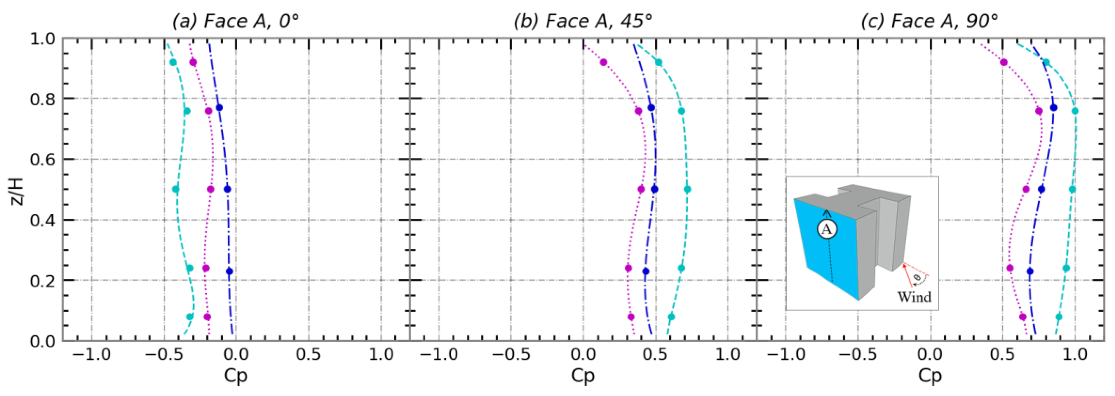
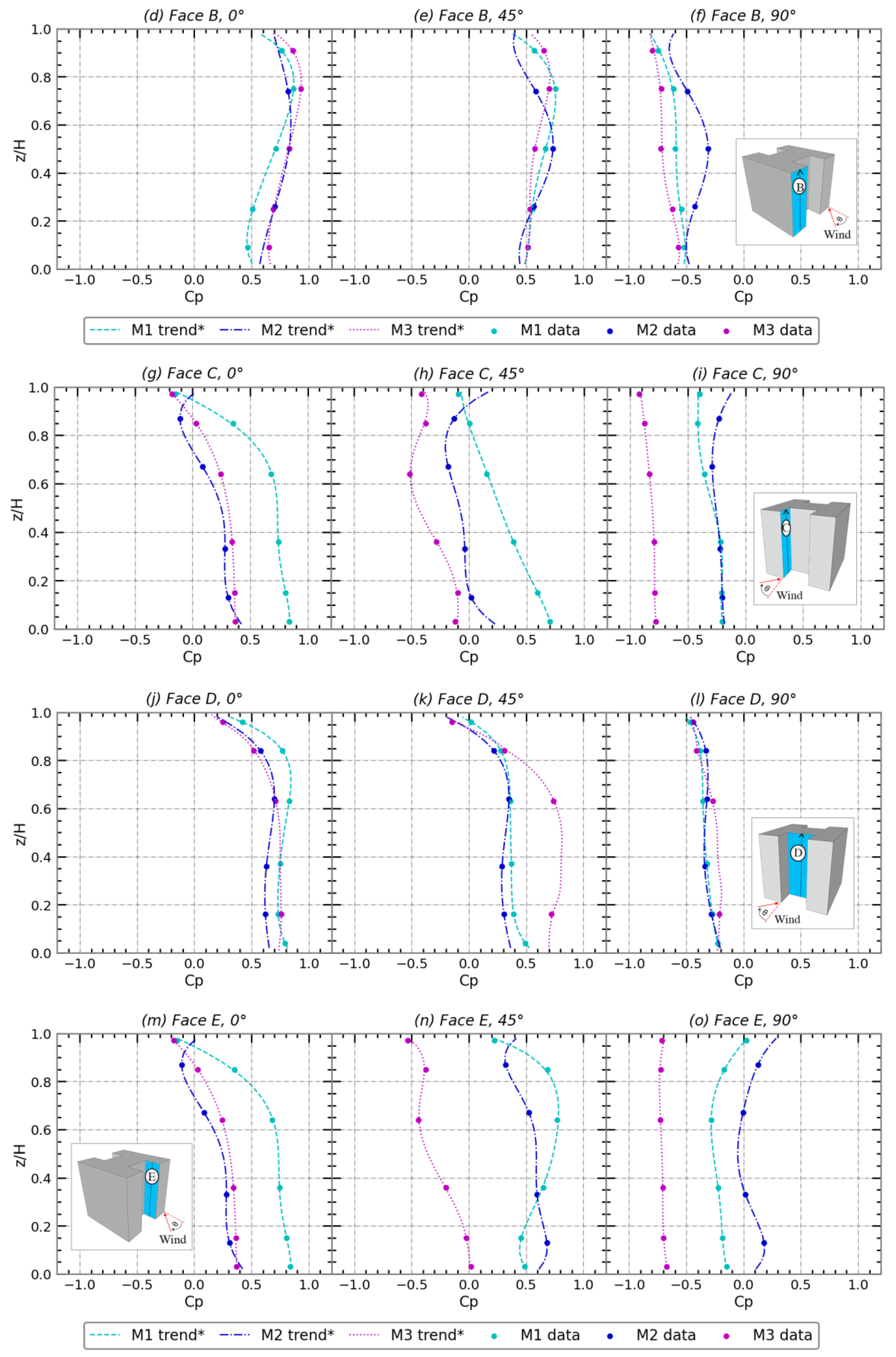
3.2. Vertical Pressure Evolution

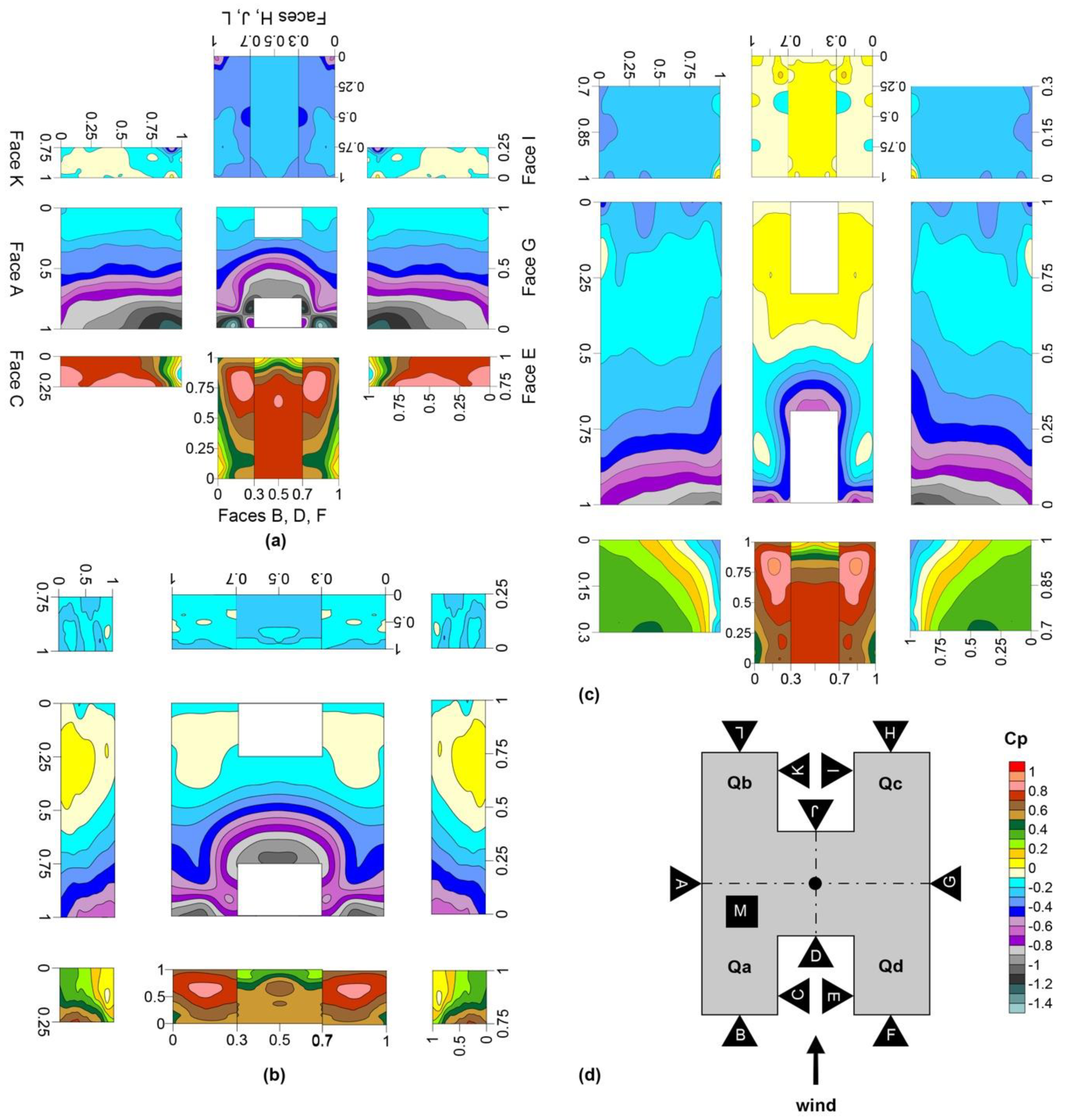
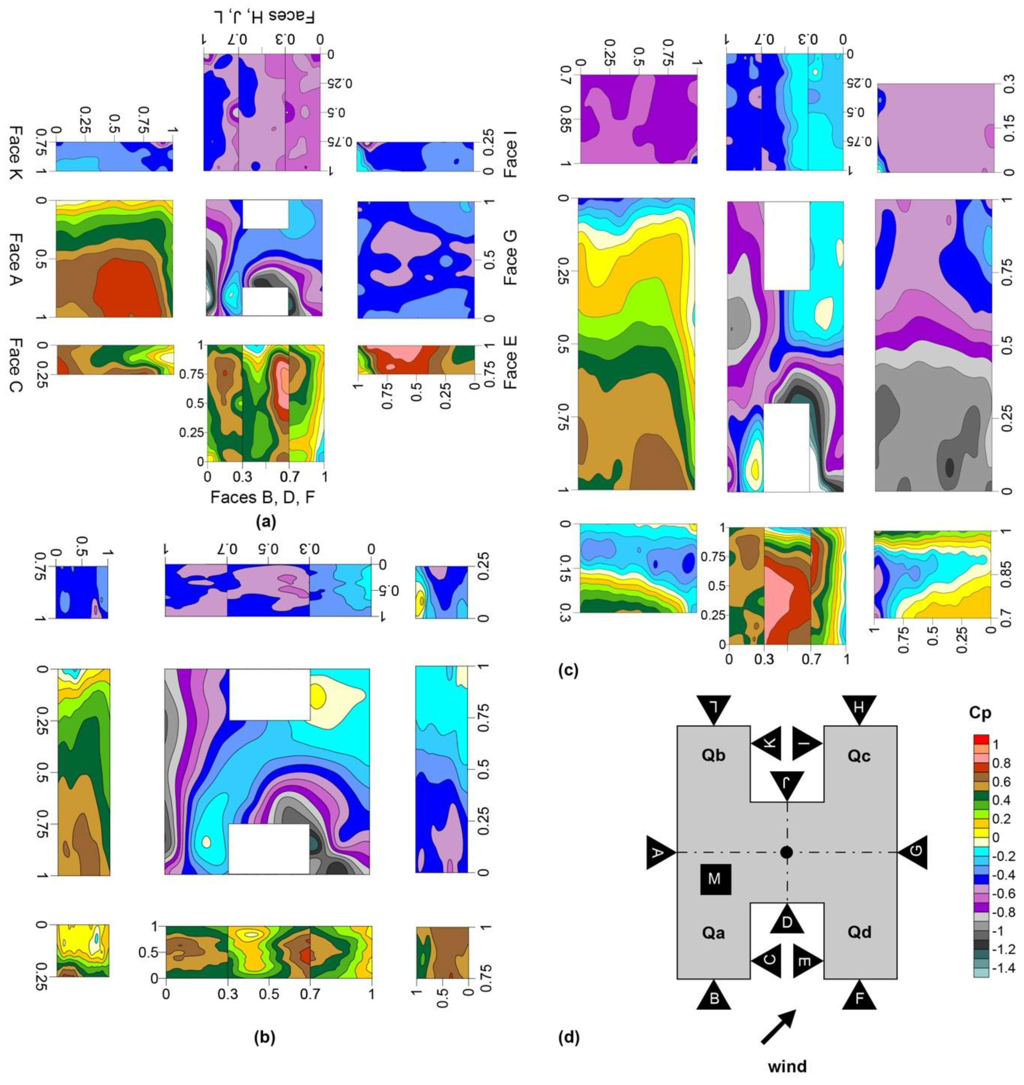
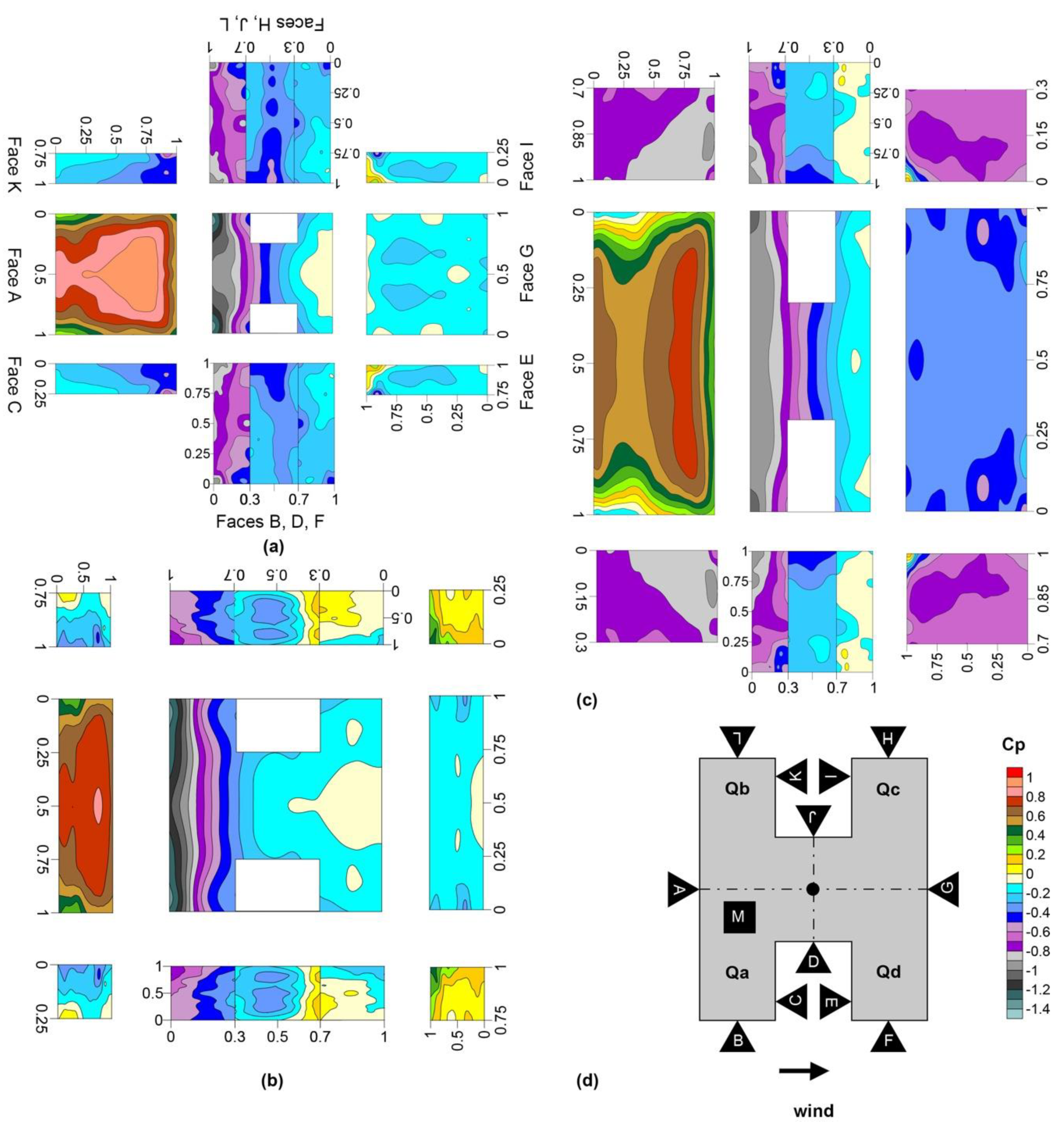
To further analyze the shape influence on the wind pressure of the study cases, the Cp distribution on the central vertical line was compared between the tested models (Figure 5). As carried out for the horizontal component, the vertical-axis data were also normalized, but in this instance, it was considered the ratio of z/H (where z= is the distance from the ground and H= is the total surface height). The vertical component displayed the Cp progression from the bottom to the top of each surface. In this section, we chose to analyze surfaces A, B, C, D, and E for 0°, 45°, and 90° wind incidences (Figure 2 identifies these surfaces in the floor plan).

Figure 5a–c presents the results for surface A, showing that near the upper edge, the Cp values decrease due to the flow deflection as it turns over the roof (for 45° and 90° wind directions), as expected for windward conditions. At the 0° angle (Figure 5a), the flow was parallel to this surface, and the Cp values were negative; furthermore, models M2 and M3 presented an average higher Cp, which was also found at the horizontal centerline (Figure 4a); this will be further analyzed when presenting the contour results (Section 3.3). However, for all other angles (Figure 5b,c) Cp is positive, as they are at direct wind incidence, and although the curve is analogous for all cases, M2 shows a smaller Cp variation, due to the lower height of the model (less wind obstruction).

Analyzing surface B at wind incidences of 0° (Figure 5d) and 45° (Figure 5e), all models had similar behaviors. For windward conditions, the pressure near the ground was approximately 0.5, and it increased until 70% of its height, where it started to decay because of the flow separation. Additionally, the proportion influences the Cp distribution at 90° (Figure 5f), since in this situation the wind obstruction is created by surface A, which is larger for M3; thus, the Cp values are lower in this study case.

Regarding surfaces C and E (sides of the models’ cavity), at 0° of wind incidence (Figure 5g,m), M1 shows more positive values due to its height and shallow cavity (as discussed in Section 3.1). However, with a 45° angle (Figure 5h,n), only M3 has negative values due to the turbulence effect; as discussed in item 1.4, there is a horizontal pressure fluctuation in these surfaces for M3, being positive at the sides and negative in the center, where the current axis is positioned. Then, at 90° wind attack (Figure 5i,o), all models presented negative Cp values, as they were located at the wake region; however, model M3 presented more negative values than others (0.6 lower), due to the cavity depth and greater obstruction created by surface A. Surface D at 0° and 90° wind attack angles (Figure 5j,l) shows analog curves; however, at 45° incidence (Figure 5k), M3 showed a higher fluctuation in Cp values, due to the displacement of the area where the wind attacks surface D. The pressure peak, has an influence on the high turbulence occurring in the deeper cavity, was also identified in the previous section.

3.3. Cp Contours

Aiming to further understand the wind pressure distribution in the case studies, the Cp contours were plotted for all surfaces of the three models, considering wind attack angles of 0°, 45°, and 90°.

At 0° incidence (Figure 6a–c), the wind impacts the windward region, flowing along the sides of the model, through the cavity, and over the roof. Inside the cavity, the wind directly impacts surface D at 60% of its height (pressure peak). From this point, the air flowed over the roof as the pressure decreased. Then, the air coming from the roof entered the posterior cavity, where indirect ventilation by suction created a negative pressure area, since it was in the wind wake zone.

Additionally, only in the M1 case study, the flow reattaches after surpassing the building (Figure 6a). This influences the pressure on its side surfaces (A and G), in which case it recovers faster than in the other models (see Section 3.1). Plus, as M2 is lower in height, the wind encounters less obstruction on the windward surfaces. Thus, upon detaching from this facade, it flows over the roof, creating less suction force; therefore, the airflow reattaches before surpassing the building. Then, in M3, although the level of obstruction encountered at the windward direction is the same as in M1, the airflow on the roof behaves similarly only up to half of its length, when it reattaches to the roof surface before surpassing the building; this phenomenon is indicated by the slightly positive pressure around 50% of M3’s length. This is due to its elongated proportion, with approximately double the length of M1 and M2.

Surface C and E of model M1 presented higher Cp values (see Figure 6a) as a result of the shallow cavity and taller model. Although M1 and M3 have the same frontal obstruction, M3 has a deeper cavity, thus creating more turbulence and reducing the pressure at its sides (surfaces C and E). As in M2, there is less obstruction, and the flow deflects to the roof more easily due to the lower obstruction in the frontal area.

Moreover, we observed differences in the lower portion of the walls between windward surfaces, at normal wind incidence. In taller buildings (M1 and M3), there is a stagnation zone that occurs at 20–30% of its height, as evident in surfaces B and D, where there is a drop in pressure in this region (Figure 6a,b). Above it, the fluid goes up and escapes through the roof. Below it, the fluid returns, creating turbulence near the ground. However, in M2, with the same wind incidence, this airflow return was not identified.

Analyzing the wind angle of 45° (Figure 7–c), the airflow entered the first cavity, forming a vortex that reached surface D between 50% and 80% of its height, where the higher pressure was found; then, the values decreased as the airflow escaped to the roof through the upper edge made by surfaces E and D. At the leeward zone, the air flowed into the leeward cavity from the roof (at the intersection of surface K and J), creating turbulence that impacted surface I at the upper portion (positive pressure—(Figure 7b)), and then leaving the recess.

Given that the M3 cavity is more than twice as deep as the other two models, the airflow continues to develop within the cavity, forming the second vortex and reversing the position where the air attacks surface D (compared to the others), (see Figure 4k and Figure 7), then escaping to the roof in the upper corner formed by surfaces C and D. Besides, Figure 7c demonstrates this vortex’s effect on surface E, showing a positive pressure on its sides (where it is impacted by the vortex) and negative pressure at the center (where the airflow retreats, creating suction). This phenomenon can be visualized in Figure 8 (scour test), where sand clear zones mean higher velocities and accumulated sand grains mean stagnation, showing the described turbulence in M1/M2 (Figure 7a) and M3. Additionally, Mandal et al. similarly observed a higher level of turbulence in C-shaped models at this wind incidence [47].

The turbulence developed in the cavity has an important influence on the pressure distribution at 0° and 45° wind attack angles, not only on its inner surfaces (C, D, and E) but also on the behavior of adjacent surfaces at windward zones (B, F, and M), as shown in Figure 6 and Figure 8. Discussing this effect on surface M (roof) at 0° and 45° wind incidence, the air flows from the windward cavity and through the roof, thus creating a negative pressure zone in the roof (surface M) near the upper edges of surface D. For 0° wind incidence, this occurs symmetrically in both edges, where there is a pressure drop, reaching a Cp of −0.8. At the 45° wind attack angle, most of the wind exits this cavity through the edge formed by surfaces D, E, and M; thus, it represents a greater volume of air and a bigger pressure drop (Cp of around −1), as shown in Figure 7.

Furthermore, surfaces B and F presented a different pattern than would be expected for the area if it did not have recesses. Since the pressure around the sides of the model (surfaces A and G) is lower than inside the cavity, there is a higher suction force directing some of the airflow around the building. This phenomenon is evidenced by the pressure distribution of M1 and M2, considering surface A with 90° wind incidence, which shows a typical pressure distribution for windward surfaces (see Figure 9a,b). Considering that models M1 and M2 have a square proportion, at an angle of 0°, surfaces B and E should have a similar pressure distribution to surface A at 90° (considering the first and last 30% portion); however, Figure 6a,b show a different pattern than Figure 9c, with a lower Cp. This change in the pressure distribution near the edges of the surfaces that encounter the cavity was also found in C-shaped models [47,48].

Examining the leeward regions, the most influential parameter was the ratio between the width and length of the shape (where the width is the windward dimension); when the length is larger than the width, the leeward surfaces have a higher Cp (a phenomenon also identified by Inan Gunaydin, T. in C-shapes [33]), since in this case the obstruction area is proportionally lower and the wind reattaches to the leeward region faster. This became clear when comparing models M1 and M3 at 0° and 90° (Figure 6a,c and Figure 9a,c).

Additionally, at 90°, the airflow attacks surface A directly and a portion of air deflects towards the sides, detaching from it and creating a negative pressure zone (wake). However, uniquely in M2, the airflow reattaches to the sides before surpassing the cavity, since the obstruction area is smaller due to the low height; this is evidenced by the positive pressure identified only in this model around 75% of the cavity width (see Figure 9b, surfaces D, E, and F, and H, I, and J).

Finally, for this wind incidence, the airflow in the cavities is very low, as they are in the wake zone. Thus, flow occurs through suction, creating a recirculation vortex, which then flows around the model sides and over the roof. Consequently, in this situation, the cavity has less influence on its adjacent surfaces; see Figure 9a–c.

4. Conclusions

This paper studied the pressure distribution of H-shaped low-rise buildings to understand the effect that shape parameters (height, proportions, and depth of the recessed cavity) have on the surface Cp distribution. To achieve this purpose, wind tunnel tests were performed with three models, and the results were presented in different levels of detail, providing in-depth data analysis. One model (M1) had unitary aspect ratios, another model (M2) had proportions to represent horizontally designed structures (such as hospital or school facilities), and the last one (M3) had dimensions to maximize the depth of the recessed cavity.

The depth of the recessed cavity influences the pressure on its inner surfaces: the sides (C and E) and the back wall (D). The side surfaces of the deeper model (M3) presented lower Cp values for oblique (45°) and perpendicular (90°) wind incidences. At windward incidence (0°), it was found that surface C of M1 has a higher Cp until 90% of its height, which is an influence of the shallow cavity and higher model. The effect of the cavity depth on surface D is clear at oblique incidence, where it displays a mirrored pressure distribution for M3. When the cavity is shallow, the peak pressure is located to the right, while with a deep cavity, it is positioned to the left; this is due to the increased turbulence that developed two vortexes in the second situation. This phenomenon also has a clear effect on surface E, showing positive pressure on its sides and negative pressure at the center.

The turbulence generated by the cavity also affected the pressure distribution of adjacent surfaces at windward direction (B, F, and M), changing the pressure distribution near the edges of the surfaces that encounter the cavity. These differences are more pronounced in M3. Furthermore, at perpendicular wind incidence, the cavity had the least impact on the pressure of the adjacent surfaces.

The building height influences the windward surfaces in its lower portion. Taller models (M1 and M3) show a stagnation zone at approximately 20–40% of their height. Above it, the wind flows to the roof, and below it, there is a recirculation vortex that modifies the pressure near the ground. However, in the model with a lower height, this recirculation was not identified. Additionally, at normal wind, the flow only reattaches after surpassing the building in M1. This influences the pressure on the model side surfaces (A and G), which recover faster, and on the windward cavity (C and E), leading to higher Cp values.

The proportion of the floor plan mainly influences the pressure on the roof (M) and lateral surfaces (A and G), as they are the wider ones. There were changes to the square floor plan distribution pattern, as usual. Otherwise, the proportion parameter influenced the leeward surfaces, considering the width-to-length ratio (where the width represents the dimension facing the wind). In cases where the length exceeded the width (low obstruction area), the downwind surfaces exhibited higher Cp values (wind reattaches faster). Furthermore, at 90°, the airflow attacks surface A directly, creating a negative pressure zone (wake) in the cavity area. In M2, there is a low obstruction to the wind, and the airflow reattaches at around 75% of the cavity width, creating a positive pressure zone.

This work’s findings show that, in most cases, there are significant differences in pressure between the cavity’s inner surfaces (C, D, and E) and surfaces in the model perimeter (A, B, F, G, H, and L). This can be used as an advantage in the design of effective natural ventilation systems, which can be beneficial, especially when the cavity is in the wake area (90° wind incidence). Also, the pressure fluctuation found in the cavity side surfaces (C and E) at 45° wind incidence can be used to generate natural ventilation between windows placed on the same surface, which is a common situation in small apartments. The study of these pressure differences for potential ventilation systems is a fertile theme for further investigation.

Therefore, the results reached corroborate the hypothesis that was initially presented: unlike the geometric dimensions of a high-rise building, the geometric dimensions of a low-rise H-shaped building can influence the pressure distribution on its surfaces, both due to its general shape (height, proportions) and the depth of the recessed cavity. Thus, applying the Cp values of rectangular buildings arbitrarily to H-shaped models in building simulations can lead to unreliable results.

We highlight that this experiment considers low-rise and isolated buildings, although neighboring buildings can affect the pressure distribution of the object. Thus, it is advisable to assess the building’s vicinity prior to applying these results to a different neighborhood situation. Additionally, this topic presents a possibility for future work.

As the research data and processing scripts are made publicly available, this work is also a valuable contribution as a primary data source for wind pressure coefficients in low-rise H-shaped buildings. These data will have a positive impact on architects and designers, as they are essential for the study of natural ventilation via the Building Energy Simulation and Airflow Network (BES-AFN).

It is important to highlight that the Cp values provided in this work are specific to the case studies presented; the use of these coefficients to simulate other proportions of the “H” may result in errors. In future works, we intend to create an extensive database through the CFD simulation validated by this study.

References

1. IPCC Summary for Policymakers. In Climate Change 2022: Mitigation of Climate Change: Working Group III to the Sixth Assessment Report of the Intergovernmental Panel on Climate Change; Al Khourdajie, A.; Hasija, A.; McCollum, D.; Lisboa, G.; Malley, J.; Belkacemi, M.; Pathak, M.; Vyas, P.; Slade, R.; Diemen, R.; et al. (Eds.) Cambridge University Press: Cambridge, UK; New York, NY, USA, 2022; p. 52. ISBN 9781107415416. [Google Scholar]
2. Rivero, R. Arquitetura e Clima; Luzzatto, D.C., Ed.; Editora da Universidade: Porto Alegre, Brazil, 1986; ISBN 9788585038441. [Google Scholar]
3. Givoni, B. Comfort, Climate Analysis and Building Design Guidelines. Energy Build. 1992, 18, 11–23. [Google Scholar] [CrossRef]
4. Rudnick, S.N.; Milton, D.K. Risk of Indoor Airborne Infection Transmission Estimated from Carbon Dioxide Concentration. Indoor Air 2003, 13, 237–245. [Google Scholar] [CrossRef] [PubMed]
5. Zemouri, C.; Awad, S.F.; Volgenant, C.M.C.; Crielaard, W.; Laheij, A.M.G.A.; de Soet, J.J. Modeling of the Transmission of Coronaviruses, Measles Virus, Influenza Virus, Mycobacterium Tuberculosis, and Legionella Pneumophila in Dental Clinics. J. Dent. Res. 2020, 99, 22034520940288. [Google Scholar] [CrossRef] [PubMed]
6. Wong, S.Y.Y.; Lam, K.M.M. Effect of Recessed Cavities on Wind-Induced Loading and Dynamic Responses of a Tall Building. J. Wind. Eng. Ind. Aerodyn. 2013, 114, 72–82. [Google Scholar] [CrossRef]
7. Teixeira, C.A.; Invidiata, A.; Sorgato, M.J.; Melo, A.P.; Fossati, M.; Lamberts, R. Levantamento Das Características de Edifícios Residenciais Brasileiros; Centro Brasileiro de Eficiência Energética em Edificações (CB3e): Florianopolis, Brazil, 2015. [Google Scholar]
8. Winiarski, D.W.; Halverson, M.A.; Jiang, W. Analysis of Building Envelope Construction in 2003 CBECS; United States Departemant of Energy: Richland, WA, USA, 2007. [Google Scholar]
9. Montes, M.A.T. Abordagem Integrada No Ciclo de Vida de Habitação de Interesse Social Considerando Mudanças Climáticas; Universidade Federal de Santa Catarina: Florianópolis, Brazil, 2016. [Google Scholar]
10. Secretaria Nacional da Habitação Sistema de Gerenciamento Da Habitação: Dados Abertos Da SNH. Available online: http://sishab.mdr.gov.br/dados_abertos/sistema_habitacao (accessed on 19 December 2022).
11. Sanketh, P.; Rao, B.D.V.C.M. Effect of Symmetrical Floor Plan Shapes with Re-Entrant Corners on Seismic Behavior of RC Buildings. i-Manag. J. Struct. Eng. 2015, 4, 15–21. [Google Scholar] [CrossRef]
12. Morais, J.M.S.C.; Labaki, L.C. Evaluating Natural Ventilation in Multi-Storey Social Housing. In Proceedings of the PLEA 2013—29th Conference, Sustainable Architecture for a Renewable Future, Munich, Germany, 10–12 September 2013. [Google Scholar]
13. Cheng, C.K.C.; Lam, K.M.; Leung, Y.T.A.; Yang, K.; Li Danny, H.W.; Cheung Sherman, C.P. Wind-Induced Natural Ventilation of Re-Entrant Bays in a High-Rise Building. J. Wind Eng. Ind. Aerodyn. 2011, 99, 79–90. [Google Scholar] [CrossRef]
14. Hong Kong Government Outbreak at the Amoy Garden. Report of the Select Committee to Inquire into the Handling of the Severe Acute Respiratory Syndrome Outbreak by the Government and the Hospital Authority; Legislative Counsil of Hong Kong: Hong Kong, China, 2004. [Google Scholar]
15. Asfour, O.S.; Gadi, M.B. A Comparison between CFD and Network Models for Predicting Wind-Driven Ventilation in Buildings. Build. Environ. 2007, 42, 4079–4085. [Google Scholar] [CrossRef]
16. Bre, F.; Gimenez, J.M. A Cloud-Based Platform to Predict Wind Pressure Coefficients on Buildings. Build. Simul. 2022, 15, 1507–1525. [Google Scholar] [CrossRef] [PubMed]
17. Cóstola, D.; Blocken, B.; Hensen, J.J.L.M.L.M.J.; Costola, D.; Blocken, B.; Hensen, J.J.L.M.L.M.J.; Cóstola, D.; Blocken, B.; Hensen, J.J.L.M.L.M.J. Overview of Pressure Coefficient Data in Building Energy Simulation and Airflow Network Programs. Build. Environ. 2009, 44, 2027–2036. [Google Scholar] [CrossRef]
18. Yuan, K.; Hui, Y.; Chen, Z. Effects of Facade Appurtenances on the Local Pressure of High-Rise Building. J. Wind Eng. Ind. Aerodyn. 2018, 178, 26–37. [Google Scholar] [CrossRef]
19. Hui, Y.; Yuan, K.; Chen, Z.; Yang, Q. Characteristics of Aerodynamic Forces on High-Rise Buildings with Various Façade Appurtenances. J. Wind Eng. Ind. Aerodyn. 2019, 191, 76–90. [Google Scholar] [CrossRef]
20. Li, B.; Liu, J.; Gao, J. Surface Wind Pressure Tests on Buildings with Various Non-Uniformity Morphological Parameters. J. Wind Eng. Ind. Aerodyn. 2015, 137, 14–24. [Google Scholar] [CrossRef]
21. Tominaga, Y.; Shirzadi, M. Wind Tunnel Measurement of Three-Dimensional Turbulent Flow Structures around a Building Group: Impact of High-Rise Buildings on Pedestrian Wind Environment. Build. Environ. 2021, 206, 108389. [Google Scholar] [CrossRef]
22. Gimenez, J.M.; Bre, F. An Enhanced K-ω SST Model to Predict Airflows around Isolated and Urban Buildings. Build. Environ. 2023, 237, 110321. [Google Scholar] [CrossRef]
23. Shelley, E.; Hubbard, E.; Zhang, W. Comparison and Uncertainty Quantification of Roof Pressure Measurements Using the NIST and TPU Aerodynamic Databases. J. Wind Eng. Ind. Aerodyn. 2023, 232, 105246. [Google Scholar] [CrossRef]
24. Li, Y.-G.Y.Y.; Liu, P.; Li, Y.-G.Y.Y.; Yan, J.-H.J.; Quan, J. Wind Loads Characteristics of Irregular Shaped High-Rise Buildings. Adv. Struct. Eng. 2022, 26, 3–16. [Google Scholar] [CrossRef]
25. Zhong, H.-Y.; Jing, Y.; Liu, Y.; Zhao, F.-Y.; Liu, D.; Li, Y. CFD Simulation of “Pumping” Flow Mechanism of an Urban Building Affected by an Upstream Building in High Reynolds Flows. Energy Build. 2019, 202, 109330. [Google Scholar] [CrossRef]
26. Albuquerque, D.P.P. de Simplified Modelling of Wind-Driven Sigle-Sided Ventilation. Ph.D. Thesis, Faculdade de Ciências da Universidade de Lisboa, Lisboa, Portugal, 2021. [Google Scholar]
27. Albuquerque, D.P.; Sandberg, M.; Linden, P.F.; Carrilho da Graça, G. Experimental and Numerical Investigation of Pumping Ventilation on the Leeward Side of a Cubic Building. Build. Environ. 2020, 179, 106897. [Google Scholar] [CrossRef]
28. Cheng, L.; Lam, K.M.; Wong, S.Y. POD Analysis of Crosswind Forces on a Tall Building with Square and H-Shaped Cross Sections. Wind Struct. 2015, 21, 63–84. [Google Scholar] [CrossRef]
29. Klein, P.; Rau, M.; Roeckle, R.; Plate, E.J. Concentration Estimation around Point Sources Located in the Vicinity of U-Shape Buildings. In Air Pollution II: Pollution Control and Monitoring; WIT Press, IT Transactions on Ecology and the Environmen: Barcelona, Spain, 1994; Volume 2, pp. 473–480. [Google Scholar]
30. Götting, J.; Winkler, C.; Rau, M.; Moussiopoulos, N.; Ernst, G. Dispersion of a Passive Pollutant in the Vicinity of a U-Shaped Building. Int. J. Environ. Pollut. 1997, 8, 718–726. [Google Scholar] [CrossRef]
31. Wang, D.; Yu, X.J.; Zhou, Y.; Tse, K.T. A Combination Method to Generate Fluctuating Boundary Conditions for Large Eddy Simulation. Wind Struct. 2015, 20, 579–607. [Google Scholar] [CrossRef]
32. Mandal, S.; Dalui, S.K.; Bhattacharjya, S. Influence of Side Ratio on Wind Induced Responses of U Plan Shape Tall Building. In Recent Trends in Civil Engineering; Lecture Notes in Civil Engineering; Springer: Singapore, 2023; Volume 274, pp. 345–355. ISBN 9789811940545. [Google Scholar]
33. Gunaydin, T.I. Numerical Study of Wind Induced Pressures on Irregular Plan Shapes. ICONARP Int. J. Archit. Plan. 2021, 9, 646–679. [Google Scholar] [CrossRef]
34. Nagar, S.K.; Raj, R.; Dev, N. Experimental Study of Wind-Induced Pressures on Tall Buildings of Different Shapes. Wind Struct. 2020, 31, 441–453. [Google Scholar] [CrossRef]
35. Ali, M.M.; Al-Kodmany, K. Tall Buildings and Urban Habitat of the 21st Century: A Global Perspective. Buildings 2012, 2, 384–423. [Google Scholar] [CrossRef]
36. Kishor, C.M.; Coulbourne, W.L. Wind Loads: Guide to the Wind Load Provisions of ASCE 7-10; American Society of Civil Engineers (ASCE): Reston, VA, USA, 2013; ISBN 978-0-7844-7778-6. [Google Scholar]
37. Wieringa, J. Updating the Davenport Roughness Classification. J. Wind Eng. Ind. Aerodyn. 1992, 41, 357–368. [Google Scholar] [CrossRef]
38. Lopes, M.F.P.; Gomes, M.G.; Ferreira, J.G. Simulation of the Atmospheric Boundary Layer for Model Testing in a Short Wind Tunnel. Exp. Tech. 2008, 32, 36–43. [Google Scholar] [CrossRef]
39. Tokyo Polytechnic University. Aerodynamic Database for Low-Rise Buildings with Varied Eaves; Tokyo Polytechnic University: Tokyo, Japan, 2007. [Google Scholar]
40. Andrioli Medinilha-Carvalho, T.; Marques da Silva, F.V.; Bre, F.; Gimenez, J.M.; Labaki, L.C. Experimental Wind Pressure Database of Low-Rise and H-Shaped Buildings (1.0) [Data Set]. 2023. Zenodo. Available online: https://zenodo.org/records/8257276 (accessed on 23 February 2024).
41. DTC Initium Utility Software, Version 2.00a; TE Connectivity: Los Angeles, CA, USA, 2017.
42. Sousa, J.H.; Gomes, M.G.; da Silva, F.M.; Tomé, A. Systematization of Spatial Functional Layouts and Pedestrian Wind Comfort Assessment for an Ultra-Thin Triangular Free Form Shell Structure. Build. Environ. 2023, 246, 110951. [Google Scholar] [CrossRef]
43. De Paepe, W.; Pindado, S.; Bram, S.; Contino, F. Simplified Elements for Wind-Tunnel Measurements with Type-III-Terrain Atmospheric Boundary Layer. Meas. J. Int. Meas. Confed. 2016, 91, 590–600. [Google Scholar] [CrossRef]
44. Morse, S.M. Wind Pressure Fields around Non-Rectangular Buildings. Master’s Thesis, Texas Tech University, Lubbock, TX, USA, 2003. [Google Scholar]
45. Surfer, version 7; Golden Software: Golden, CO, USA, 1999.
46. Spyder, version 5.1.5; Python Software Foundation: Wilmington, DE, USA, 2020.
47. Andrioli Medinilha-Carvalho, T.; Marques da Silva, F.V.; Bre, F.; Gimenez, J.M.; Labaki, L.C. Automated Data Processing Script for Wind Tunnel Measurements in Python (1.0). Zenodo. 2023. Available online: https://zenodo.org/records/8247854 (accessed on 23 February 2024).
48. Inan Gunaydin, T. Wind Flow on and around U-Shaped Buildings. J. Eng. Des. Technol. 2022, 20, 841–859. [Google Scholar] [CrossRef]
Figure 1. Picture of the three physical models: (a) M1, (b) M2, and (c) M3.
Buildings 14 00762 g001
Figure 2. Geometry characterization of H-shaped models. (a) Floor-plan model parameterization, quadrant divisions, and surface names (no scale); (b) 3D model; and (c) models’ dimensions in meters.
Buildings 14 00762 g002
Figure 3. ABL wind profile: measured turbulence intensity and velocity. * Power trend was applied.
Buildings 14 00762 g003
Figure 4. Pressure coefficients along the horizontal centerline (H/2) for the 3 tested models: (a) Face A, 0°, (b) Face A, 45, (c) Face A, 90°, (d) Face B, 0°, (e) Face B, 45°, (f) Face B, 90°, (g) Face C, 0°, (h) Face C, 45°, (i) Face C, 90°, (j) Face D, 0°, (k) Face D, 45°, (l) Face D, 90°, (m) Face E, 0°, (n) Face E, 45°, and (o) Face E, 90°. * Trend was computed using a polynomial function of fifth degree.
Buildings 14 00762 g004aBuildings 14 00762 g004b
Figure 5. Pressure coefficients along the vertical centerline (X/2) for the 3 tested models: (a) Face A, 0°, (b) Face A, 45, (c) Face A, 90°, (d) Face B, 0°, (e) Face B, 45°, (f) Face B, 90°, (g) Face C, 0°, (h) Face C, 45°, (i) Face C, 90°, (j) Face D, 0°, (k) Face D, 45°, (l) Face D, 90°, (m) Face E, 0°, (n) Face E, 45°, and (o) Face E, 90°. * Trend was computed using a polynomial function of fifth degree.
Buildings 14 00762 g005aBuildings 14 00762 g005b
Figure 6. Cp contour distribution of the three models for θ = 0°. (a) M1; (b) M2; (c) M3; (d) model’s floor-plan schematics indicating quadrant divisions and surface names (no scale).
Buildings 14 00762 g006
Figure 7. Cp contour distribution of the three models for θ = 45°. (a) M1; (b) M2; (c) M3; (d) model’s floor-plan schematics indicating quadrant divisions and surface names (no scale).
Buildings 14 00762 g007
Figure 8. Superposition of sand experiment photograph and floor plan representing the wind flow schematics over the models’ cavity, at ground level. (a) Shallow cavities (M1 and M2); (b) deep cavity (M3). The wind attack angle is 45°. * Indicates a break of undefined length within a drawing.
Buildings 14 00762 g008
Figure 9. Cp contour distribution on the three models for θ = 90°. (a) M1; (b) M2; (c) M3; (d) model’s floor-plan schematics indicating quadrant divisions and surface names (no scale).
Buildings 14 00762 g009
Disclaimer/Publisher’s Note: The statements, opinions and data contained in all publications are solely those of the individual author(s) and contributor(s) and not of MDPI and/or the editor(s). MDPI and/or the editor(s) disclaim responsibility for any injury to people or property resulting from any ideas, methods, instructions or products referred to in the content.