
Transfer-Learning Prediction Model for Low-Cycle Fatigue Life of Bimetallic Steel Bars

Abstract
:1. Introduction
2. Experimental Results from Fatigue Experiment
2.1. Test Approach
2.2. Variables
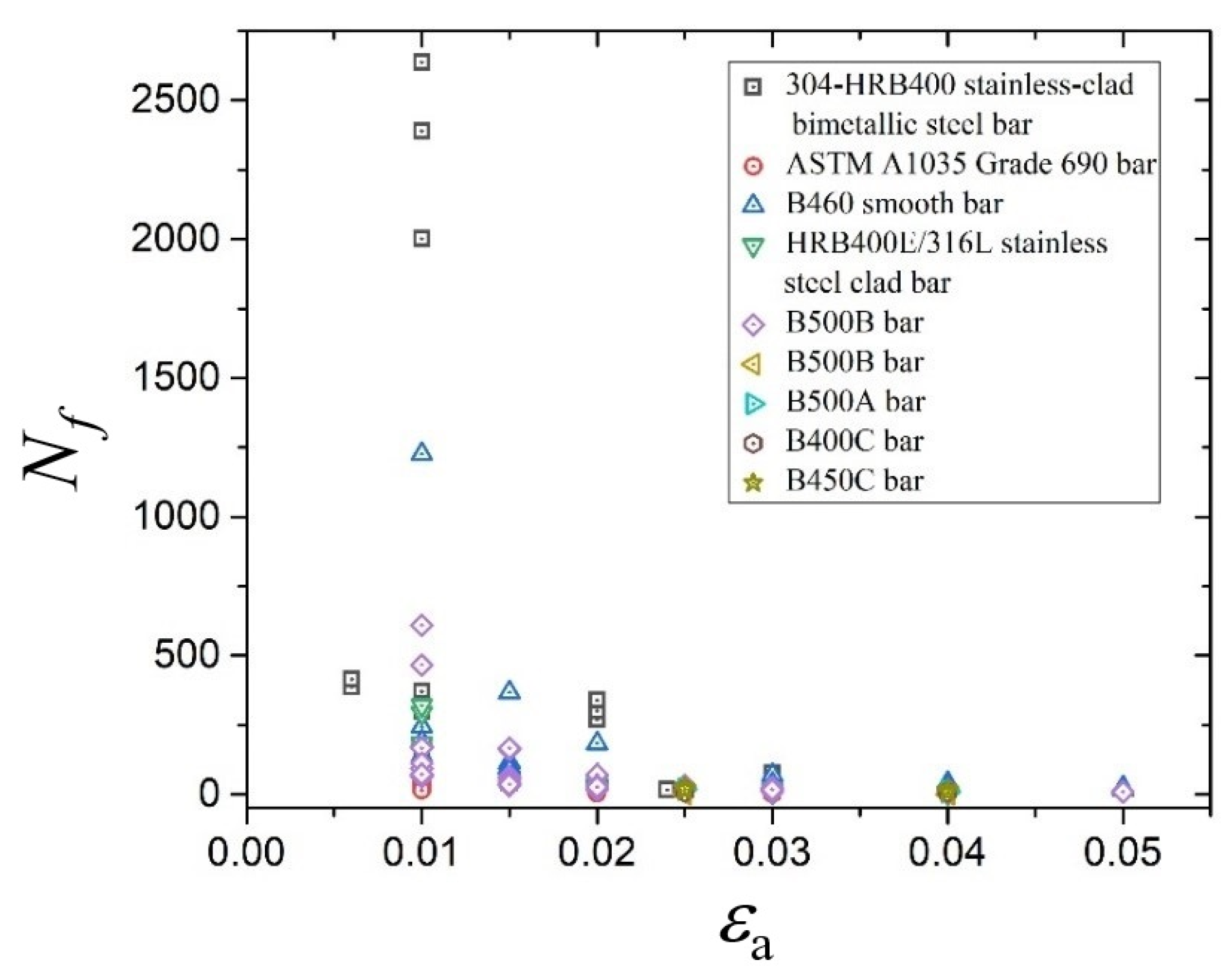
2.3. Dataset of Experimental Data
3. Framework
3.1. Performance Metrics
3.2. Construction of Source Model
3.2.1. Neural Network Architecture
3.2.2. Model Training and Hyperparameter Tuning
3.3. Construction of Transfer Model
4. Results
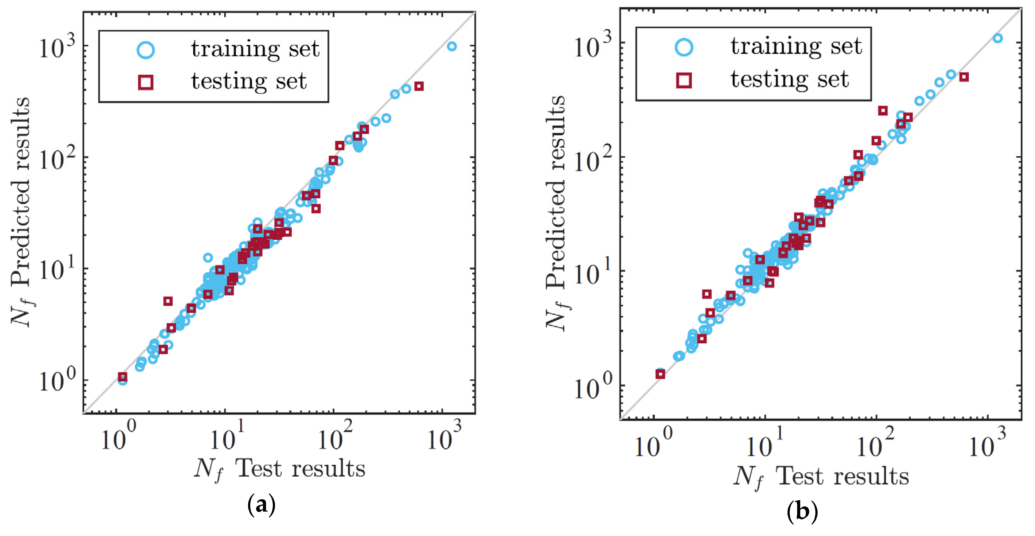
4.1. Prediction Results for Source Models
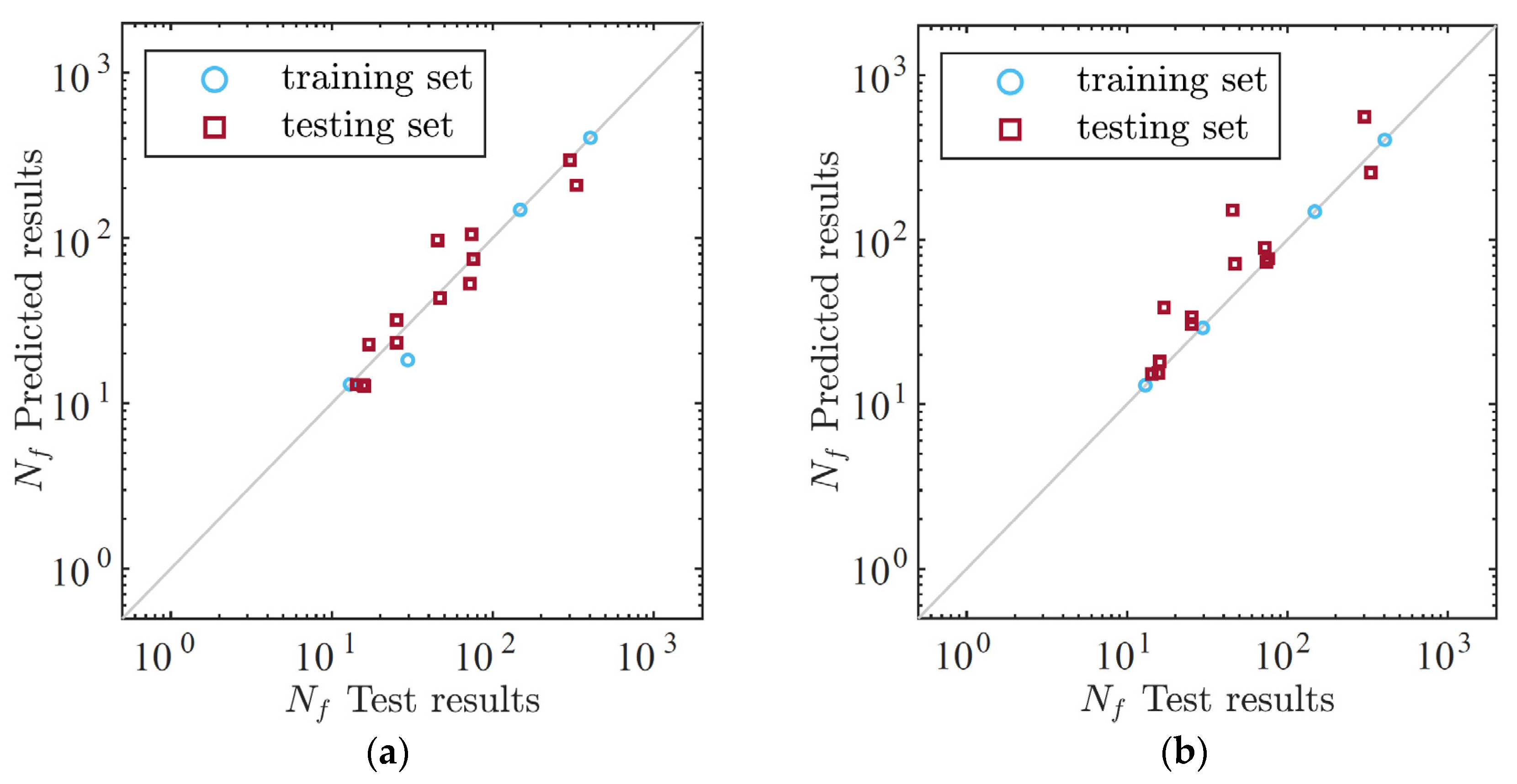
4.2. Prediction Results for Transfer Models
5. Discussion
5.1. Efficiency of the Transfer Framework
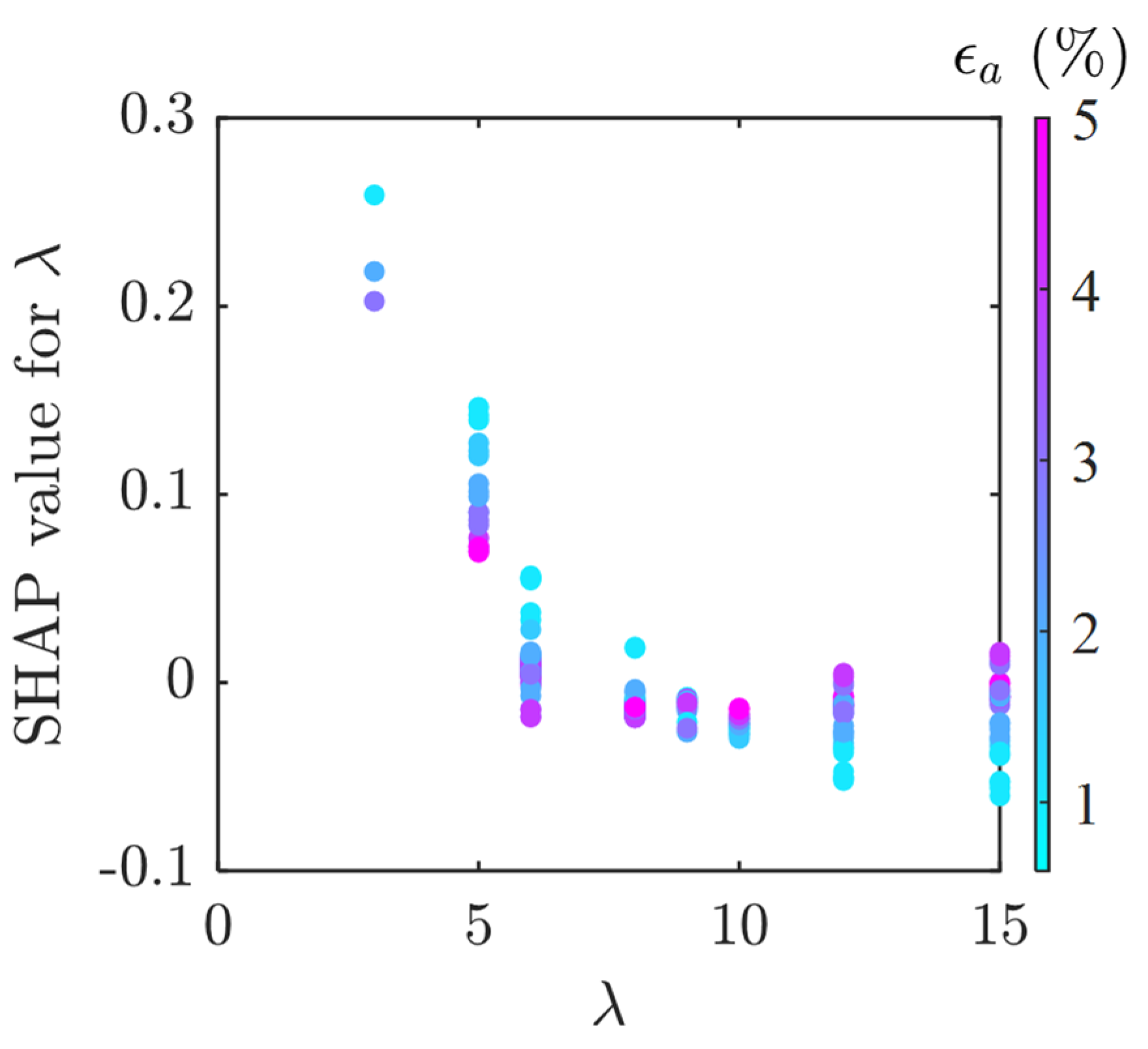
5.2. Influence of Key Parameters
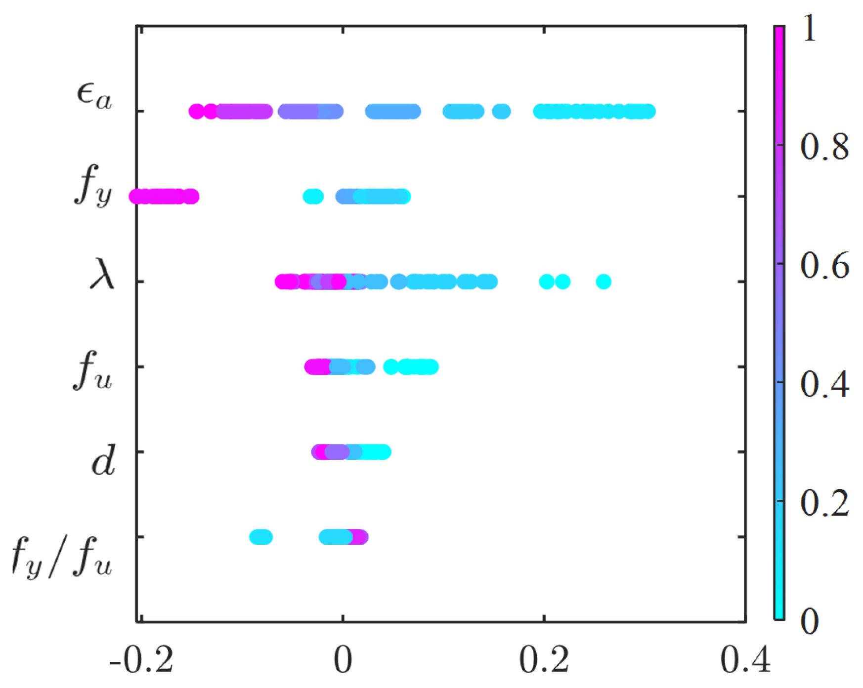
5.3. The Relative Importance of Features on the Fatigue Life
5.4. Limitations and Prospects
6. Conclusions
Author Contributions
Funding
Data Availability Statement
Conflicts of Interest
Appendix A

| Number | Type | λ | d (mm) | εa | fy (MPa) | fu (MPa) | Nf |
|---|---|---|---|---|---|---|---|
| T-6-0.006 | 304-HRB400 stainless-clad bimetallic steel bar [22] | 6 | 18 | 0.60% | 486.15 | 652.52 | 410 |
| T-6-0.006 | 6 | 18 | 0.60% | 486.15 | 652.52 | 387 | |
| T-6-0.006 | 6 | 18 | 0.60% | 486.15 | 652.52 | 415 | |
| T-6-0.015 | 6 | 18 | 1.50% | 486.15 | 652.52 | 50 | |
| T-6-0.015 | 6 | 18 | 1.50% | 486.15 | 652.52 | 42 | |
| T-6-0.015 | 6 | 18 | 1.50% | 486.15 | 652.52 | 44 | |
| T-6-0.024 | 6 | 18 | 2.40% | 486.15 | 652.52 | 17 | |
| T-6-0.024 | 6 | 18 | 2.40% | 486.15 | 652.52 | 18 | |
| T-6-0.024 | 6 | 18 | 2.40% | 486.15 | 652.52 | 16 | |
| T-3-0.01 | 3 | 18 | 1.00% | 486.15 | 652.52 | 2390 | |
| T-3-0.01 | 3 | 18 | 1.00% | 486.15 | 652.52 | 2001 | |
| T-3-0.01 | 3 | 18 | 1.00% | 486.15 | 652.52 | 2637 | |
| T-6-0.01 | 6 | 18 | 1.00% | 486.15 | 652.52 | 370 | |
| T-6-0.01 | 6 | 18 | 1.00% | 486.15 | 652.52 | 297 | |
| T-6-0.01 | 6 | 18 | 1.00% | 486.15 | 652.52 | 325 | |
| T-9-0.01 | 9 | 18 | 1.00% | 486.15 | 652.52 | 164 | |
| T-9-0.01 | 9 | 18 | 1.00% | 486.15 | 652.52 | 144 | |
| T-9-0.01 | 9 | 18 | 1.00% | 486.15 | 652.52 | 136 | |
| T-12-0.01 | 12 | 18 | 1.00% | 486.15 | 652.52 | 76 | |
| T-12-0.01 | 12 | 18 | 1.00% | 486.15 | 652.52 | 73 | |
| T-12-0.01 | 12 | 18 | 1.00% | 486.15 | 652.52 | 72 | |
| T-15-0.01 | 15 | 18 | 1.00% | 486.15 | 652.52 | 76 | |
| T-15-0.01 | 15 | 18 | 1.00% | 486.15 | 652.52 | 71 | |
| T-15-0.01 | 15 | 18 | 1.00% | 486.15 | 652.52 | 80 | |
| T-3-0.02 | 3 | 18 | 2.00% | 486.15 | 652.52 | 269 | |
| T-3-0.02 | 3 | 18 | 2.00% | 486.15 | 652.52 | 300 | |
| T-3-0.02 | 3 | 18 | 2.00% | 486.15 | 652.52 | 339 | |
| T-6-0.02 | 6 | 18 | 2.00% | 486.15 | 652.52 | 47 | |
| T-6-0.02 | 6 | 18 | 2.00% | 486.15 | 652.52 | 46 | |
| T-6-0.02 | 6 | 18 | 2.00% | 486.15 | 652.52 | 48 | |
| T-9-0.02 | 9 | 18 | 2.00% | 486.15 | 652.52 | 31 | |
| T-9-0.02 | 9 | 18 | 2.00% | 486.15 | 652.52 | 23 | |
| T-9-0.02 | 9 | 18 | 2.00% | 486.15 | 652.52 | 22 | |
| T-12-0.02 | 12 | 18 | 2.00% | 486.15 | 652.52 | 28 | |
| T-12-0.02 | 12 | 18 | 2.00% | 486.15 | 652.52 | 25 | |
| T-12-0.02 | 12 | 18 | 2.00% | 486.15 | 652.52 | 23 | |
| T-15-0.02 | 15 | 18 | 2.00% | 486.15 | 652.52 | 26 | |
| T-15-0.02 | 15 | 18 | 2.00% | 486.15 | 652.52 | 34 | |
| T-15-0.02 | 15 | 18 | 2.00% | 486.15 | 652.52 | 29 | |
| T-3-0.03 | 3 | 18 | 3.00% | 486.15 | 652.52 | 71 | |
| T-3-0.03 | 3 | 18 | 3.00% | 486.15 | 652.52 | 70 | |
| T-3-0.03 | 3 | 18 | 3.00% | 486.15 | 652.52 | 76 | |
| T-6-0.03 | 6 | 18 | 3.00% | 486.15 | 652.52 | 14 | |
| T-6-0.03 | 6 | 18 | 3.00% | 486.15 | 652.52 | 17 | |
| T-6-0.03 | 6 | 18 | 3.00% | 486.15 | 652.52 | 17 | |
| T-9-0.03 | 9 | 18 | 3.00% | 486.15 | 652.52 | 13 | |
| T-9-0.03 | 9 | 18 | 3.00% | 486.15 | 652.52 | 13 | |
| T-9-0.03 | 9 | 18 | 3.00% | 486.15 | 652.52 | 13 | |
| T-12-0.03 | 12 | 18 | 3.00% | 486.15 | 652.52 | 12 | |
| T-12-0.03 | 12 | 18 | 3.00% | 486.15 | 652.52 | 14 | |
| T-12-0.03 | 12 | 18 | 3.00% | 486.15 | 652.52 | 17 | |
| T-15-0.03 | 15 | 18 | 3.00% | 486.15 | 652.52 | 18 | |
| T-15-0.03 | 15 | 18 | 3.00% | 486.15 | 652.52 | 15 | |
| T-15-0.03 | 15 | 18 | 3.00% | 486.15 | 652.52 | 14 | |
| 12.7-6db-0.01 (1) | ASTM A1035 Grade 690 [5] | 6 | 12.7 | 1.00% | 795.5 | 1054.65 | 49 |
| 12.7-6db-0.01 (2) | 6 | 12.7 | 1.00% | 795.5 | 1054.65 | 44 | |
| 12.7-6db-0.02 (1) | 6 | 12.7 | 2.00% | 795.5 | 1054.65 | 4 | |
| 12.7-6db-0.02 (2) | 6 | 12.7 | 2.00% | 795.5 | 1054.65 | 4 | |
| 12.7-6db-0.03 (1) | 6 | 12.7 | 3.00% | 795.5 | 1054.65 | 1 | |
| 12.7-6db-0.03 (2) | 6 | 12.7 | 3.00% | 795.5 | 1054.65 | 2 | |
| 12.7-6db-0.04 (1) | 6 | 12.7 | 4.00% | 795.5 | 1054.65 | 1 | |
| 12.7-6db-0.04 (2) | 6 | 12.7 | 4.00% | 795.5 | 1054.65 | 1 | |
| 12.7-9db-0.01 (1) | 9 | 12.7 | 1.00% | 795.5 | 1054.65 | 30 | |
| 12.7-9db-0.01 (2) | 9 | 12.7 | 1.00% | 795.5 | 1054.65 | 28 | |
| 12.7-9db-0.02 (1) | 9 | 12.7 | 2.00% | 795.5 | 1054.65 | 4 | |
| 12.7-9db-0.02 (2) | 9 | 12.7 | 2.00% | 795.5 | 1054.65 | 3 | |
| 12.7-9db-0.03 (1) | 9 | 12.7 | 3.00% | 795.5 | 1054.65 | 2 | |
| 12.7-9db-0.03 (2) | 9 | 12.7 | 3.00% | 795.5 | 1054.65 | 2 | |
| 12.7-9db-0.04 (1) | 9 | 12.7 | 4.00% | 795.5 | 1054.65 | 2 | |
| 12.7-9db-0.04 (2) | 9 | 12.7 | 4.00% | 795.5 | 1054.65 | 2 | |
| 12.7-12db-0.01 (1) | 12 | 12.7 | 1.00% | 795.5 | 1054.65 | 15 | |
| 12.7-12db-0.01 (2) | 12 | 12.7 | 1.00% | 795.5 | 1054.65 | 17 | |
| 12.7-12db-0.02 (1) | 12 | 12.7 | 2.00% | 795.5 | 1054.65 | 4 | |
| 12.7-12db-0.02 (2) | 12 | 12.7 | 2.00% | 795.5 | 1054.65 | 4 | |
| 12.7-12db-0.03 (1) | 12 | 12.7 | 3.00% | 795.5 | 1054.65 | 3 | |
| 12.7-12db-0.03 (2) | 12 | 12.7 | 3.00% | 795.5 | 1054.65 | 2 | |
| 12.7-12db-0.04 (1) | 12 | 12.7 | 4.00% | 795.5 | 1054.65 | 2 | |
| 12.7-12db-0.04 (2) | 12 | 12.7 | 4.00% | 795.5 | 1054.65 | 2 | |
| 12.7-15db-0.01 (1) | 15 | 12.7 | 1.00% | 795.5 | 1054.65 | 15 | |
| 12.7-15db-0.01 (2) | 15 | 12.7 | 1.00% | 795.5 | 1054.65 | 14 | |
| 12.7-15db-0.02 (1) | 15 | 12.7 | 2.00% | 795.5 | 1054.65 | 5 | |
| 12.7-15db-0.02 (2) | 15 | 12.7 | 2.00% | 795.5 | 1054.65 | 5 | |
| 12.7-15db-0.03 (1) | 15 | 12.7 | 3.00% | 795.5 | 1054.65 | 3 | |
| 12.7-15db-0.03 (2) | 15 | 12.7 | 3.00% | 795.5 | 1054.65 | 3 | |
| 12.7-15db-0.04 (1) | 15 | 12.7 | 4.00% | 795.5 | 1054.65 | 3 | |
| 12.7-15db-0.04 (2) | 15 | 12.7 | 4.00% | 795.5 | 1054.65 | 3 | |
| 15.88-6db-0.01 (1) | 6 | 15.88 | 1.00% | 774 | 1017.3 | 48 | |
| 15.88-6db-0.01 (2) | 6 | 15.88 | 1.00% | 774 | 1017.3 | 31 | |
| 15.88-6db-0.02 (1) | 6 | 15.88 | 2.00% | 774 | 1017.3 | 3 | |
| 15.88-6db-0.02 (2) | 6 | 15.88 | 2.00% | 774 | 1017.3 | 5 | |
| 15.88-6db-0.03 (1) | 6 | 15.88 | 3.00% | 774 | 1017.3 | 2 | |
| 15.88-6db-0.03 (2) | 6 | 15.88 | 3.00% | 774 | 1017.3 | 1 | |
| 15.88-6db-0.04 (1) | 6 | 15.88 | 4.00% | 774 | 1017.3 | 1 | |
| 15.88-6db-0.04 (2) | 6 | 15.88 | 4.00% | 774 | 1017.3 | 1 | |
| 15.88-9db-0.01 (1) | 9 | 15.88 | 1.00% | 774 | 1017.3 | 27 | |
| 15.88-9db-0.01 (2) | 9 | 15.88 | 1.00% | 774 | 1017.3 | 23 | |
| 15.88-9db-0.02 (1) | 9 | 15.88 | 2.00% | 774 | 1017.3 | 3 | |
| 15.88-9db-0.02 (2) | 9 | 15.88 | 2.00% | 774 | 1017.3 | 4 | |
| 15.88-9db-0.03 (1) | 9 | 15.88 | 3.00% | 774 | 1017.3 | 2 | |
| 15.88-9db-0.03 (2) | 9 | 15.88 | 3.00% | 774 | 1017.3 | 2 | |
| 15.88-9db-0.04 (1) | 9 | 15.88 | 4.00% | 774 | 1017.3 | 2 | |
| 15.88-9db-0.04 (2) | 9 | 15.88 | 4.00% | 774 | 1017.3 | 1 | |
| 15.88-12db-0.01 (1) | 12 | 15.88 | 1.00% | 774 | 1017.3 | 15 | |
| 15.88-12db-0.01 (2) | 12 | 15.88 | 1.00% | 774 | 1017.3 | 17 | |
| 15.88-12db-0.02 (1) | 12 | 15.88 | 2.00% | 774 | 1017.3 | 6 | |
| 15.88-12db-0.02 (2) | 12 | 15.88 | 2.00% | 774 | 1017.3 | 4 | |
| 15.88-12db-0.03 (1) | 12 | 15.88 | 3.00% | 774 | 1017.3 | 3 | |
| 15.88-12db-0.03 (2) | 12 | 15.88 | 3.00% | 774 | 1017.3 | 2 | |
| 15.88-12db-0.04 (1) | 12 | 15.88 | 4.00% | 774 | 1017.3 | 2 | |
| 15.88-12db-0.04 (2) | 12 | 15.88 | 4.00% | 774 | 1017.3 | 2 | |
| 15.88-15db-0.01 (1) | 15 | 15.88 | 1.00% | 774 | 1017.3 | 14 | |
| 15.88-15db-0.01 (2) | 15 | 15.88 | 1.00% | 774 | 1017.3 | 14 | |
| 15.88-15db-0.02 (1) | 15 | 15.88 | 2.00% | 774 | 1017.3 | 4 | |
| 15.88-15db-0.02 (2) | 15 | 15.88 | 2.00% | 774 | 1017.3 | 5 | |
| 15.88-15db-0.03 (1) | 15 | 15.88 | 3.00% | 774 | 1017.3 | 3 | |
| 15.88-15db-0.03 (2) | 15 | 15.88 | 3.00% | 774 | 1017.3 | 3 | |
| 15.88-15db-0.04 (1) | 15 | 15.88 | 4.00% | 774 | 1017.3 | 2 | |
| 15.88-15db-0.04 (2) | 15 | 15.88 | 4.00% | 774 | 1017.3 | 3 | |
| B460-5d-0.01 | B460 smooth bar [50] | 5 | 12 | 1.00% | 474.5 | 510.564 | 1226 |
| B460-10d-0.01 | 10 | 12 | 1.00% | 474.5 | 510.564 | 243 | |
| B460-12d-0.01 | 12 | 12 | 1.00% | 474.5 | 510.564 | 192 | |
| B460-15d-0.01 | 15 | 12 | 1.00% | 474.5 | 510.564 | 140 | |
| B460-5d-0.015 | 5 | 12 | 1.50% | 474.5 | 510.564 | 367 | |
| B460-8d-0.015 | 8 | 12 | 1.50% | 474.5 | 510.564 | 115 | |
| B460-10d-0.015 | 10 | 12 | 1.50% | 474.5 | 510.564 | 100 | |
| B460-12d-0.015 | 12 | 12 | 1.50% | 474.5 | 510.564 | 94 | |
| B460-15d-0.015 | 15 | 12 | 1.50% | 474.5 | 510.564 | 85 | |
| B460-5d-0.02 | 5 | 12 | 2.00% | 474.5 | 510.564 | 184 | |
| B460-8d-0.02 | 8 | 12 | 2.00% | 474.5 | 510.564 | 69 | |
| B460-10d-0.02 | 10 | 12 | 2.00% | 474.5 | 510.564 | 64 | |
| B460-12d-0.02 | 12 | 12 | 2.00% | 474.5 | 510.564 | 58 | |
| B460-15d-0.02 | 15 | 12 | 2.00% | 474.5 | 510.564 | 52 | |
| B460-5d-0.03 | 5 | 12 | 3.00% | 474.5 | 510.564 | 69 | |
| B460-8d-0.03 | 8 | 12 | 3.00% | 474.5 | 510.564 | 38 | |
| B460-10d-0.03 | 10 | 12 | 3.00% | 474.5 | 510.564 | 37 | |
| B460-12d-0.03 | 12 | 12 | 3.00% | 474.5 | 510.564 | 32 | |
| B460-15d-0.03 | 15 | 12 | 3.00% | 474.5 | 510.564 | 32 | |
| B460-5d-0.04 | 5 | 12 | 4.00% | 474.5 | 510.564 | 40 | |
| B460-8d-0.04 | 8 | 12 | 4.00% | 474.5 | 510.564 | 23 | |
| B460-10d-0.04 | 10 | 12 | 4.00% | 474.5 | 510.564 | 22 | |
| B460-12d-0.04 | 12 | 12 | 4.00% | 474.5 | 510.564 | 22 | |
| B460-15d-0.04 | 15 | 12 | 4.00% | 474.5 | 510.564 | 24 | |
| B460-5d-0.05 | 5 | 12 | 5.00% | 474.5 | 510.564 | 26 | |
| B460-8d-0.05 | 8 | 12 | 5.00% | 474.5 | 510.564 | 17 | |
| B460-10d-0.05 | 10 | 12 | 5.00% | 474.5 | 510.564 | 17 | |
| B460-12d-0.05 | 12 | 12 | 5.00% | 474.5 | 510.564 | 17 | |
| B460-15d-0.05 | 15 | 12 | 5.00% | 474.5 | 510.564 | 18 | |
| FSC14S2.0R0.1(1) | HRB400E/316L stainless steel clad bar [3] | 6 | 14 | 1.00% | 466.5 | 661 | 175 |
| FSC14S2.0R0.1(2) | 6 | 14 | 1.00% | 466.5 | 661 | 159 | |
| FSC14S4.0R0.1(1) | 6 | 14 | 2.00% | 466.5 | 661 | 24 | |
| FSC14S4.0R0.1(2) | 6 | 14 | 2.00% | 466.5 | 661 | 23 | |
| FSC14S6.0R0.1(1) | 6 | 14 | 3.00% | 466.5 | 661 | 6 | |
| FSC14S6.0R0.1(2) | 6 | 14 | 3.00% | 466.5 | 661 | 6 | |
| FSC14S8.0R0.1(1) | 6 | 14 | 4.00% | 466.5 | 661 | 3 | |
| FSC14S8.0R0.1(2) | 6 | 14 | 4.00% | 466.5 | 661 | 3 | |
| FSC18S2.0R0.1(1) | 6 | 18 | 1.00% | 474.6 | 645 | 181 | |
| FSC18S2.0R0.1(2) | 6 | 18 | 1.00% | 474.6 | 645 | 183 | |
| FSC18S4.0R0.1(1) | 6 | 18 | 2.00% | 474.6 | 645 | 22 | |
| FSC18S4.0R0.1(2) | 6 | 18 | 2.00% | 474.6 | 645 | 18 | |
| FSC18S6.0R0.1(1) | 6 | 18 | 3.00% | 474.6 | 645 | 9 | |
| FSC18S6.0R0.1(2) | 6 | 18 | 3.00% | 474.6 | 645 | 7 | |
| FSC18S8.0R0.1(1) | 6 | 18 | 4.00% | 474.6 | 645 | 6 | |
| FSC18S8.0R0.1(2) | 6 | 18 | 4.00% | 474.6 | 645 | 5 | |
| FSC25S2.0R0.1(1) | 6 | 25 | 1.00% | 495.5 | 662.1 | 292 | |
| FSC25S2.0R0.1(2) | 6 | 25 | 1.00% | 495.5 | 662.1 | 319 | |
| FSC25S4.0R0.1(1) | 6 | 25 | 2.00% | 495.5 | 662.1 | 31 | |
| FSC25S4.0R0.1(2) | 6 | 25 | 2.00% | 495.5 | 662.1 | 35 | |
| FSC25S6.0R0.1(1) | 6 | 25 | 3.00% | 495.5 | 662.1 | 13 | |
| FSC25S6.0R0.1(2) | 6 | 25 | 3.00% | 495.5 | 662.1 | 18 | |
| FSC25S8.0R0.1(1) | 6 | 25 | 4.00% | 495.5 | 662.1 | 6 | |
| FSC25S8.0R0.1(2) | 6 | 25 | 4.00% | 495.5 | 662.1 | 6 | |
| B500B-5d-0.01 | B500B bar [50] | 5 | 16 | 1.00% | 535.67 | 633.75 | 609 |
| B500B-8d-0.01 | 8 | 16 | 1.00% | 535.67 | 633.75 | 171 | |
| B500B-10d-0.01 | 10 | 16 | 1.00% | 535.67 | 633.75 | 92 | |
| B500B-12d-0.01 | 12 | 16 | 1.00% | 535.67 | 633.75 | 68 | |
| B500B-15d-0.01 | 15 | 16 | 1.00% | 535.67 | 633.75 | 62 | |
| B500B-5d-0.015 | 5 | 16 | 1.50% | 535.67 | 633.75 | 162 | |
| B500B-8d-0.015 | 8 | 16 | 1.50% | 535.67 | 633.75 | 57 | |
| B500B-10d-0.015 | 10 | 16 | 1.50% | 535.67 | 633.75 | 33 | |
| B500B-12d-0.015 | 12 | 16 | 1.50% | 535.67 | 633.75 | 32 | |
| B500B-15d-0.015 | 15 | 16 | 1.50% | 535.67 | 633.75 | 31 | |
| B500B-5d-0.02 | 5 | 16 | 2.00% | 535.67 | 633.75 | 66 | |
| B500B-8d-0.02 | 8 | 16 | 2.00% | 535.67 | 633.75 | 23 | |
| B500B-10d-0.02 | 10 | 16 | 2.00% | 535.67 | 633.75 | 22 | |
| B500B-12d-0.02 | 12 | 16 | 2.00% | 535.67 | 633.75 | 25 | |
| B500B-15d-0.02 | 15 | 16 | 2.00% | 535.67 | 633.75 | 19 | |
| B500B-5d-0.025 | 5 | 16 | 2.50% | 535.67 | 633.75 | 32 | |
| B500B-8d-0.025 | 8 | 16 | 2.50% | 535.67 | 633.75 | 15 | |
| B500B-10d-0.025 | 10 | 16 | 2.50% | 535.67 | 633.75 | 14 | |
| B500B-12d-0.025 | 12 | 16 | 2.50% | 535.67 | 633.75 | 14 | |
| B500B-15d-0.025 | 15 | 16 | 2.50% | 535.67 | 633.75 | 16 | |
| B500B-5d-0.03 | 5 | 16 | 3.00% | 535.67 | 633.75 | 24 | |
| B500B-8d-0.03 | 8 | 16 | 3.00% | 535.67 | 633.75 | 11 | |
| B500B-10d-0.03 | 10 | 16 | 3.00% | 535.67 | 633.75 | 11 | |
| B500B-12d-0.03 | 12 | 16 | 3.00% | 535.67 | 633.75 | 11 | |
| B500B-15d-0.03 | 15 | 16 | 3.00% | 535.67 | 633.75 | 13 | |
| B500B-5d-0.04 | 5 | 16 | 4.00% | 535.67 | 633.75 | 13 | |
| B500B-8d-0.04 | 8 | 16 | 4.00% | 535.67 | 633.75 | 7 | |
| B500B-10d-0.04 | 10 | 16 | 4.00% | 535.67 | 633.75 | 7 | |
| B500B-12d-0.04 | 12 | 16 | 4.00% | 535.67 | 633.75 | 9 | |
| B500B-15d-0.04 | 15 | 16 | 4.00% | 535.67 | 633.75 | 9 | |
| B500B-5d-0.01 | 5 | 12 | 1.00% | 544.33 | 640.67 | 467 | |
| B500B-8d-0.01 | 8 | 12 | 1.00% | 544.33 | 640.67 | 167 | |
| B500B-10d-0.01 | 10 | 12 | 1.00% | 544.33 | 640.67 | 111 | |
| B500B-12d-0.01 | 12 | 12 | 1.00% | 544.33 | 640.67 | 74 | |
| B500B-15d-0.01 | 15 | 12 | 1.00% | 544.33 | 640.67 | 72 | |
| B500B-5d-0.015 | 5 | 12 | 1.50% | 544.33 | 640.67 | 166 | |
| B500B-8d-0.015 | 8 | 12 | 1.50% | 544.33 | 640.67 | 64 | |
| B500B-10d-0.015 | 10 | 12 | 1.50% | 544.33 | 640.67 | 50 | |
| B500B-12d-0.015 | 12 | 12 | 1.50% | 544.33 | 640.67 | 41 | |
| B500B-15d-0.015 | 15 | 12 | 1.50% | 544.33 | 640.67 | 36 | |
| B500B-5d-0.02 | 5 | 12 | 2.00% | 544.33 | 640.67 | 71 | |
| B500B-8d-0.02 | 8 | 12 | 2.00% | 544.33 | 640.67 | 32 | |
| B500B-10d-0.02 | 10 | 12 | 2.00% | 544.33 | 640.67 | 26 | |
| B500B-12d-0.02 | 12 | 12 | 2.00% | 544.33 | 640.67 | 23 | |
| B500B-15d-0.02 | 15 | 12 | 2.00% | 544.33 | 640.67 | 27 | |
| B500B-5d-0.03 | 5 | 12 | 3.00% | 544.33 | 640.67 | 26 | |
| B500B-8d-0.03 | 8 | 12 | 3.00% | 544.33 | 640.67 | 15 | |
| B500B-10d-0.03 | 10 | 12 | 3.00% | 544.33 | 640.67 | 13 | |
| B500B-12d-0.03 | 12 | 12 | 3.00% | 544.33 | 640.67 | 19 | |
| B500B-15d-0.03 | 15 | 12 | 3.00% | 544.33 | 640.67 | 17 | |
| B500B-5d-0.04 | 5 | 12 | 4.00% | 544.33 | 640.67 | 17 | |
| B500B-8d-0.04 | 8 | 12 | 4.00% | 544.33 | 640.67 | 12 | |
| B500B-10d-0.04 | 10 | 12 | 4.00% | 544.33 | 640.67 | 9 | |
| B500B-12d-0.04 | 12 | 12 | 4.00% | 544.33 | 640.67 | 14 | |
| B500B-15d-0.04 | 15 | 12 | 4.00% | 544.33 | 640.67 | 12 | |
| B500B-5d-0.05 | 5 | 12 | 5.00% | 544.33 | 640.67 | 10 | |
| B500B-8d-0.05 | 8 | 12 | 5.00% | 544.33 | 640.67 | 8 | |
| B500B-10d-0.05 | 10 | 12 | 5.00% | 544.33 | 640.67 | 8 | |
| B500B-12d-0.05 | 12 | 12 | 5.00% | 544.33 | 640.67 | 8 | |
| B500B-15d-0.05 | 15 | 12 | 5.00% | 544.33 | 640.67 | 9 | |
| B500B-16-TEMP Prod.1.1 | B500B bar [51] | 6 | 16 | 2.50% | 596.6 | 671.4 | 19 |
| B500B-16-TEMP Prod.1.1 | 6 | 16 | 4.00% | 596.6 | 671.4 | 8 | |
| B500B-16-TEMP Prod.1.1 | 8 | 16 | 2.50% | 596.6 | 671.4 | 15 | |
| B500B-16-TEMP Prod.1.1 | 8 | 16 | 4.00% | 596.6 | 671.4 | 10 | |
| B500B-16-TEMP Prod.1.2 | 6 | 16 | 2.50% | 572 | 668.3 | 19 | |
| B500B-16-TEMP Prod.1.2 | 6 | 16 | 4.00% | 572 | 668.3 | 8 | |
| B500B-16-TEMP Prod.1.2 | 8 | 16 | 2.50% | 572 | 668.3 | 15 | |
| B500B-16-TEMP Prod.1.2 | 8 | 16 | 4.00% | 572 | 668.3 | 6 | |
| B500B-16-TEMP Prod.1.3 | 6 | 16 | 2.50% | 513.1 | 616.3 | 19 | |
| B500B-16-TEMP Prod.1.3 | 6 | 16 | 4.00% | 513.1 | 616.3 | 9 | |
| B500B-16-TEMP Prod.1.3 | 8 | 16 | 2.50% | 513.1 | 616.3 | 13 | |
| B500B-16-TEMP Prod.1.3 | 8 | 16 | 4.00% | 513.1 | 616.3 | 8 | |
| B500B-16-TEMP Prod.2 | 6 | 16 | 2.50% | 516.9 | 635 | 20 | |
| B500B-16-TEMP Prod.2 | 6 | 16 | 4.00% | 516.9 | 635 | 11 | |
| B500B-16-TEMP Prod.2 | 8 | 16 | 2.50% | 516.9 | 635 | 14 | |
| B500B-16-TEMP Prod.2 | 8 | 16 | 4.00% | 516.9 | 635 | 7 | |
| B500B-20-TEMP Prod.2 | 6 | 20 | 2.50% | 515.3 | 621.8 | 20 | |
| B500B-20-TEMP Prod.2 | 6 | 20 | 4.00% | 515.3 | 621.8 | 9 | |
| B500B-20-TEMP Prod.2 | 8 | 20 | 2.50% | 515.3 | 621.8 | 16 | |
| B500B-20-TEMP Prod.2 | 8 | 20 | 4.00% | 515.3 | 621.8 | 7 | |
| B500B-8-STR Prod.1 | 6 | 8 | 2.50% | 565.6 | 619.3 | 20 | |
| B500B-8-STR Prod.1 | 6 | 8 | 4.00% | 565.6 | 619.3 | 11 | |
| B500B-8-STR Prod.1 | 8 | 8 | 2.50% | 565.6 | 619.3 | 20 | |
| B500B-8-STR Prod.1 | 8 | 8 | 4.00% | 565.6 | 619.3 | 10 | |
| B500B-8-TEMP Prod.2 | 6 | 8 | 2.50% | 584.7 | 671.5 | 20 | |
| B500B-8-TEMP Prod.2 | 6 | 8 | 4.00% | 584.7 | 671.5 | 11 | |
| B500B-8-TEMP Prod.2 | 8 | 8 | 2.50% | 584.7 | 671.5 | 17 | |
| B500B-8-TEMP Prod.2 | 8 | 8 | 4.00% | 584.7 | 671.5 | 9 | |
| B500B-12-STR Prod.1 | 6 | 12 | 2.50% | 538.4 | 627 | 25 | |
| B500B-12-STR Prod.1 | 6 | 12 | 4.00% | 538.4 | 627 | 8 | |
| B500B-12-STR Prod.1 | 8 | 12 | 2.50% | 538.4 | 627 | 15 | |
| B500B-12-STR Prod.1 | 8 | 12 | 4.00% | 538.4 | 627 | 7 | |
| B500A-8-CW Prod.2 | B500A bar [51] | 6 | 8 | 2.50% | 526.4 | 546.8 | 20 |
| B500A-8-CW Prod.2 | 6 | 8 | 4.00% | 526.4 | 546.8 | 14 | |
| B500A-8-CW Prod.2 | 8 | 8 | 2.50% | 526.4 | 546.8 | 19 | |
| B500A-8-CW Prod.2 | 8 | 8 | 4.00% | 526.4 | 546.8 | 12 | |
| B500A-12-CW Prod.2 | 6 | 12 | 2.50% | 567.7 | 589 | 20 | |
| B500A-12-CW Prod.2 | 6 | 12 | 4.00% | 567.7 | 589 | 8 | |
| B500A-12-CW Prod.2 | 8 | 12 | 2.50% | 567.7 | 589 | 17 | |
| B500A-12-CW Prod.2 | 8 | 12 | 4.00% | 567.7 | 589 | 8 | |
| B400C-8-TEMP Prod.1 | B400C bar [51] | 6 | 8 | 2.50% | 442.9 | 567.3 | 20 |
| B400C-8-TEMP Prod.1 | 6 | 8 | 4.00% | 442.9 | 567.3 | 12 | |
| B400C-8-TEMP Prod.1 | 8 | 8 | 2.50% | 442.9 | 567.3 | 20 | |
| B400C-8-TEMP Prod.1 | 8 | 8 | 4.00% | 442.9 | 567.3 | 12 | |
| B400C-16-MA Prod.2 | 6 | 16 | 2.50% | 434.5 | 565.3 | 20 | |
| B400C-16-MA Prod.2 | 6 | 16 | 4.00% | 434.5 | 565.3 | 12 | |
| B400C-16-MA Prod.2 | 8 | 16 | 2.50% | 434.5 | 565.3 | 17 | |
| B400C-16-MA Prod.2 | 8 | 16 | 4.00% | 434.5 | 565.3 | 8 | |
| B400C-20-MA Prod.2 | 6 | 20 | 2.50% | 416 | 563.3 | 20 | |
| B400C-20-MA Prod.2 | 6 | 20 | 4.00% | 416 | 563.3 | 9 | |
| B400C-20-MA Prod.2 | 8 | 20 | 2.50% | 416 | 563.3 | 18 | |
| B400C-20-MA Prod.2 | 8 | 20 | 4.00% | 416 | 563.3 | 9 | |
| B400C-20-TEMP Prod.2 | 6 | 20 | 2.50% | 436.2 | 557.2 | 20 | |
| B400C-20-TEMP Prod.2 | 6 | 20 | 4.00% | 436.2 | 557.2 | 7 | |
| B400C-20-TEMP Prod.2 | 8 | 20 | 2.50% | 436.2 | 557.2 | 7 | |
| B450C-8-STR Prod.1 | B450C bar [51] | 6 | 8 | 2.50% | 530.2 | 624.8 | 20 |
| B450C-8-STR Prod.1 | 6 | 8 | 4.00% | 530.2 | 624.8 | 15 | |
| B450C-8-STR Prod.1 | 8 | 8 | 2.50% | 530.2 | 624.8 | 20 | |
| B450C-8-STR Prod.1 | 8 | 8 | 4.00% | 530.2 | 624.8 | 16 | |
| B450C-12-STR Prod.1 | 6 | 12 | 2.50% | 530.2 | 619.6 | 28 | |
| B450C-12-STR Prod.1 | 6 | 12 | 4.00% | 530.2 | 619.6 | 9 | |
| B450C-12-STR Prod.1 | 8 | 12 | 2.50% | 530.2 | 619.6 | 18 | |
| B450C-12-STR Prod.1 | 8 | 12 | 4.00% | 530.2 | 619.6 | 8 | |
| B450C-12-STR Prod.2 | 6 | 12 | 2.50% | 513.8 | 599.7 | 20 | |
| B450C-12-STR Prod.2 | 6 | 12 | 4.00% | 513.8 | 599.7 | 14 | |
| B450C-12-STR Prod.2 | 8 | 12 | 2.50% | 513.8 | 599.7 | 20 | |
| B450C-12-STR Prod.2 | 8 | 12 | 4.00% | 513.8 | 599.7 | 12 | |
| B450C-16-TEMP Prod.1.1 | 6 | 16 | 2.50% | 537.3 | 640.5 | 19 | |
| B450C-16-TEMP Prod.1.1 | 6 | 16 | 4.00% | 537.3 | 640.5 | 9 | |
| B450C-16-TEMP Prod.1.1 | 8 | 16 | 2.50% | 537.3 | 640.5 | 13 | |
| B450C-16-TEMP Prod.1.1 | 8 | 16 | 4.00% | 537.3 | 640.5 | 11 | |
| B450C-16-TEMP Prod.1.2 | 6 | 16 | 2.50% | 446.7 | 542.7 | 18 | |
| B450C-16-TEMP Prod.1.2 | 6 | 16 | 4.00% | 446.7 | 542.7 | 18 | |
| B450C-16-TEMP Prod.1.2 | 8 | 16 | 2.50% | 446.7 | 542.7 | 18 | |
| B450C-16-TEMP Prod.1.2 | 8 | 16 | 4.00% | 446.7 | 542.7 | 9 | |
| B450C-16-TEMP Prod.1.3 | 6 | 16 | 2.50% | 517.8 | 615.4 | 19 | |
| B450C-16-TEMP Prod.1.3 | 6 | 16 | 4.00% | 517.8 | 615.4 | 14 | |
| B450C-16-TEMP Prod.1.3 | 8 | 16 | 2.50% | 517.8 | 615.4 | 15 | |
| B450C-16-TEMP Prod.1.3 | 8 | 16 | 4.00% | 517.8 | 615.4 | 9 | |
| B450C-16-TEMP Prod.2 | 6 | 16 | 2.50% | 479.3 | 601.1 | 18 | |
| B450C-16-TEMP Prod.2 | 6 | 16 | 4.00% | 479.3 | 601.1 | 8 | |
| B450C-16-TEMP Prod.2 | 8 | 16 | 2.50% | 479.3 | 601.1 | 18 | |
| B450C-16-TEMP Prod.2 | 8 | 16 | 4.00% | 479.3 | 601.1 | 7 | |
| B450C-20-TEMP Prod.2 | 6 | 20 | 2.50% | 492.9 | 591.4 | 19 | |
| B450C-20-TEMP Prod.2 | 6 | 20 | 4.00% | 492.9 | 591.4 | 7 | |
| B450C-20-TEMP Prod.2 | 8 | 20 | 2.50% | 492.9 | 591.4 | 19 | |
| B450C-20-TEMP Prod.2 | 8 | 20 | 4.00% | 492.9 | 591.4 | 7 |
References
- Wang, N.; Zhou, F.; Xu, H.; Xu, Z. Seismic behaviour of flat connections between steel-plate composite (SC) walls and reinforced concrete (RC) walls. J. Constr. Steel Res. 2020, 168, 105929. [Google Scholar] [CrossRef]
- Wang, N.; Zhou, F.; Li, Z.; Xu, Z.; Xu, H. Experimental and numerical investigation on the L-joint composed of steel-plate composite (SC) walls under seismic loading. Eng. Struct. 2021, 227, 111360. [Google Scholar] [CrossRef]
- Li, W.; Wang, Q.; Qu, H.; Xiang, Y.; Li, Z. Mechanical properties of HRB400E/316L stainless steel clad rebar under low-cycle fatigue. Structures 2022, 38, 292–305. [Google Scholar] [CrossRef]
- Deng, Z.; Huang, S.; Wang, Y.; Xue, H. Experimental research on fatigue behavior of prestressed ultra-high performance concrete beams with high-strength steel bars. Structures 2022, 43, 1778–1789. [Google Scholar] [CrossRef]
- Aldabagh, S.; Alam, M.S. Low-cycle fatigue performance of high-strength steel reinforcing bars considering the effect of inelastic buckling. Eng. Struct. 2021, 235, 112114. [Google Scholar] [CrossRef]
- Apostolopoulos, C.A. Mechanical behavior of corroded reinforcing steel bars S500s tempcore under low cycle fatigue. Constr. Build. Mater. 2007, 21, 1447–1456. [Google Scholar] [CrossRef]
- Hawileh, R.; Rahman, A.; Tabatabai, H. Evaluation of the Low-Cycle Fatigue Life in ASTM A706 and A615 Grade 60 Steel Reinforcing Bars. J. Mater. Civ. Eng. 2010, 22, 65–76. [Google Scholar] [CrossRef]
- Kashani, M.M.; Alagheband, P.; Khan, R.; Davis, S. Impact of corrosion on low-cycle fatigue degradation of reinforcing bars with the effect of inelastic buckling. Int. J. Fatigue 2015, 77, 174–185. [Google Scholar] [CrossRef]
- Hua, J.; Wang, F.; Huang, L.; Wang, N.; Xue, X. Experimental study on mechanical properties of corroded stainless-clad bimetallic steel bars. Constr. Build. Mater. 2021, 287, 123019. [Google Scholar] [CrossRef]
- Hua, J.; Wang, F.; Wang, N.; Huang, L.; Hai, L.; Li, Y.; Zhu, X.; Xue, X. Experimental and numerical investigations on corroded stainless-clad bimetallic steel bar with artificial damage. J. Build. Eng. 2021, 44, 102779. [Google Scholar] [CrossRef]
- Shi, Y.; Luo, Z.; Zhou, X.; Xue, X.; Li, J. Post-fire mechanical properties of titanium–clad bimetallic steel in different cooling approaches. J. Constr. Steel Res. 2022, 191, 107169. [Google Scholar] [CrossRef]
- Shi, Y.; Luo, Z.; Zhou, X.; Xue, X.; Xiang, Y. Post-fire performance of bonding interface in explosion-welded stainless-clad bimetallic steel. J. Constr. Steel Res. 2022, 193, 107285. [Google Scholar] [CrossRef]
- Xue, X.; Hua, J.; Wang, F.; Wang, N.; Li, S. Mechanical Property Model of Q620 High-Strength Steel with Corrosion Effects. Buildings 2022, 12, 1651. [Google Scholar] [CrossRef]
- He, Z.; Shen, A.; Wang, W.; Zuo, X.; Wu, J. Evaluation and optimization of various treatment methods for enhancing the properties of brick-concrete recycled coarse aggregate. J. Adhes. Sci. Technol. 2022, 36, 1060–1080. [Google Scholar] [CrossRef]
- Hua, J.; Wang, F.; Yang, Z.; Xue, X.; Huang, L.; Chen, Z. Low-cycle fatigue properties of bimetallic steel bars after exposure to elevated temperature. J. Constr. Steel Res. 2021, 187, 106959. [Google Scholar] [CrossRef]
- Hua, J.; Wang, F.; Xiang, Y.; Yang, Z.; Xue, X.; Huang, L.; Wang, N. Mechanical properties of stainless-clad bimetallic steel bars exposed to elevated temperatures. Fire Saf. J. 2022, 127, 103521. [Google Scholar] [CrossRef]
- Hua, J.; Yang, Z.; Wang, F.; Xue, X.; Wang, N.; Huang, L. Relation between the metallographic structure and mechanical properties of a bimetallic steel bar after fire. J. Mater. Civ. Eng. 2022, 34, 04022193. [Google Scholar] [CrossRef]
- Hua, J.; Yang, Z.; Xue, X.; Huang, L.; Wang, N.; Chen, Z. Bond properties of bimetallic steel bar in seawater sea-sand concrete at different ages. Constr. Build. Mater. 2022, 323, 126539. [Google Scholar] [CrossRef]
- Liu, G.; Hua, J.; Wang, N.; Deng, W.; Xue, X. Material Alternatives for Concrete Structures on Remote Islands: Based on Life-cycle cost Analysis. Adv. Civ. Eng. 2022, 2022, 7329408. [Google Scholar] [CrossRef]
- Hua, J.; Fan, H.; Yan, W.; Wang, N.; Xue, X.; Huang, L. Seismic resistance of the corroded bimetallic steel bar under different strain amplitudes. Constr. Build. Mater. 2022, 319, 126088. [Google Scholar] [CrossRef]
- Hua, J.; Wang, F.; Xue, X.; Fan, H.; Yan, W. Fatigue properties of bimetallic steel bar: An experimental and numerical study. Eng. Fail. Anal. 2022, 136, 106212. [Google Scholar] [CrossRef]
- Wang, F.; Hua, J.; Xue, X.; Ding, Z.; Lyu, Y.; Liu, Q. Low-cycle fatigue performance of bimetallic steel bar considering the effect of inelastic buckling. Constr. Build. Mater. 2022, 351, 128787. [Google Scholar] [CrossRef]
- Xiao, L.; Li, Q.Y.; Li, H.; Ren, Q. Loading capacity prediction and optimization of cold-formed steel built-up section columns based on machine learning methods. Thin-Walled Struct. 2022, 180, 109826. [Google Scholar] [CrossRef]
- Xiao, L.; Hua, J.; Li, H.; Xue, X.; Wang, N.; Wang, F. Quantitative analysis on post–fire–resistant performance of high–strength steel plate girders using LSTM. J. Constr. Steel Res. 2022, 199, 107588. [Google Scholar] [CrossRef]
- Feng, D.-C.; Li, Y.; Shafieezadeh, A.; Taciroglu, E. Advances in Data-Driven Risk-Based Performance Assessment of Structures and Infrastructure Systems. J. Struct. Eng. 2023, 149, 2022–2023. [Google Scholar] [CrossRef]
- Cardellicchio, A.; Ruggieri, S.; Nettis, A.; Renò, V.; Uva, G. Physical interpretation of machine learning-based recognition of defects for the risk management of existing bridge heritage. Eng. Fail. Anal. 2023, 149, 107237. [Google Scholar] [CrossRef]
- Jafari, A.; Ma, L.Y.; Shahmansouri, A.A.; Dugnani, R. Quantitative fractography for brittle fracture via multilayer perceptron neural network. Eng. Fract. Mech. 2023, 291, 109545. [Google Scholar] [CrossRef]
- Bao, H.; Wu, S.; Wu, Z.; Kang, G.; Peng, X.; Withers, P.J. A machine-learning fatigue life prediction approach of additively manufactured metals. Eng. Fract. Mech. 2021, 242, 107508. [Google Scholar] [CrossRef]
- Yang, J.; Kang, G.; Liu, Y.; Chen, K.; Kan, Q. Life prediction for rate-dependent low-cycle fatigue of PA6 polymer considering ratchetting: Semi-empirical model and neural network based approach. Int. J. Fatigue 2020, 136, 105619. [Google Scholar] [CrossRef]
- Srinivasan, V.S.; Valsan, M.; Rao, K.B.S.; Mannan, S.L.; Raj, B. Low cycle fatigue and creep–fatigue interaction behavior of 316L(N) stainless steel and life prediction by artificial neural network approach. Int. J. Fatigue 2003, 25, 1327–1338. [Google Scholar] [CrossRef]
- Vassilopoulos, A.P.; Georgopoulos, E.F.; Dionysopoulos, V. Artificial neural networks in spectrum fatigue life prediction of composite materials. Int. J. Fatigue 2007, 29, 20–29. [Google Scholar] [CrossRef]
- Zhan, Z.; Li, H. Machine learning based fatigue life prediction with effects of additive manufacturing process parameters for printed SS 316L. Int. J. Fatigue 2021, 142, 105941. [Google Scholar] [CrossRef]
- Zhan, Z.; Li, H. A novel approach based on the elastoplastic fatigue damage and machine learning models for life prediction of aerospace alloy parts fabricated by additive manufacturing. Int. J. Fatigue 2021, 145, 106089. [Google Scholar] [CrossRef]
- He, L.; Wang, Z.; Akebono, H.; Sugeta, A. Machine learning-based predictions of fatigue life and fatigue limit for steels. J. Mater. Sci. Technol. 2021, 90, 9–19. [Google Scholar] [CrossRef]
- Zhang, X.-C.; Gong, J.-G.; Xuan, F.-Z. A deep learning based life prediction method for components under creep, fatigue and creep-fatigue conditions. Int. J. Fatigue 2021, 148, 106236. [Google Scholar] [CrossRef]
- Yang, J.; Kang, G.; Liu, Y.; Kan, Q. A novel method of multiaxial fatigue life prediction based on deep learning. Int. J. Fatigue 2021, 151, 106356. [Google Scholar] [CrossRef]
- Kamiyama, M.; Shimizu, K.; Akiniwa, Y. Prediction of low-cycle fatigue crack development of sputtered Cu thin film using deep convolutional neural network. Int. J. Fatigue 2022, 162, 106998. [Google Scholar] [CrossRef]
- Chen, J.; Liu, Y. Probabilistic physics-guided machine learning for fatigue data analysis. Expert Syst. Appl. 2021, 168, 114316. [Google Scholar] [CrossRef]
- Guo, X.; Liu, X.; Long, G.; Zhao, Y.; Yuan, Y. Data-driven prediction of the fatigue performance of corroded high-strength steel wires. Eng. Fail. Anal. 2023, 146, 107108. [Google Scholar] [CrossRef]
- Pan, S.J.; Yang, Q. A Survey on Transfer Learning. IEEE Trans. Knowl. Data Eng. 2010, 22, 1345–1359. [Google Scholar] [CrossRef]
- Weiss, K.; Khoshgoftaar, T.M.; Wang, D.D. A Survey of Transfer Learning; Springer International Publishing: Berlin/Heidelberg, Germany, 2016. [Google Scholar] [CrossRef]
- Kaya, A.; Keceli, A.S.; Catal, C.; Yalic, H.Y.; Temucin, H.; Tekinerdogan, B. Analysis of transfer learning for deep neural network based plant classification models. Comput. Electron. Agric. 2019, 158, 20–29. [Google Scholar] [CrossRef]
- He, R.; Tian, Z.G.; Zuo, M.J. A transferable neural network method for remaining useful life prediction. Mech. Syst. Signal Process. 2023, 183, 109608. [Google Scholar] [CrossRef]
- Yin, T.; Lu, N.; Guo, G.S.; Lei, Y.G.; Wang, S.H.; Guan, X.H. Knowledge and data dual-driven transfer network for industrial robot fault diagnosis. Mech. Syst. Signal Process. 2023, 182, 109597. [Google Scholar] [CrossRef]
- Wei, X.; Zhang, C.; Han, S.; Jia, Z.; Wang, C.; Xu, W. High cycle fatigue S-N curve prediction of steels based on transfer learning guided long short term memory network. Int. J. Fatigue 2022, 163, 107050. [Google Scholar] [CrossRef]
- Kashani, M.M.; Crewe, A.J.; Alexander, N.A. Nonlinear stress-strain behaviour of corrosion-damaged reinforcing bars including inelastic buckling. Eng. Struct. 2013, 48, 417–429. [Google Scholar] [CrossRef]
- Tripathi, M.; Dhakal, R.P.; Dashti, F.; Massone, L.M. Low-cycle fatigue behaviour of reinforcing bars including the effect of inelastic buckling. Constr. Build. Mater. 2018, 190, 1226–1235. [Google Scholar] [CrossRef]
- Hu, M.; Han, Q.; Xu, K.; Du, X. Corrosion influences on monotonic properties of ultra-high-strength reinforcing steels. Constr. Build. Mater. 2019, 198, 82–97. [Google Scholar] [CrossRef]
- Hua, J.; Wang, F.; Xue, X.; Ding, Z.; Chen, Z. Residual monotonic mechanical properties of bimetallic steel bar with fatigue damage. J. Build. Eng. 2022, 55, 104703. [Google Scholar] [CrossRef]
- Kashani, M.M.; Barmi, A.K.; Malinova, V.S. Influence of inelastic buckling on low-cycle fatigue degradation of reinforcing bars. Constr. Build. Mater. 2015, 94, 644–655. [Google Scholar] [CrossRef]
- Caprili, S.; Salvatore, W. Cyclic behaviour of uncorroded and corroded steel reinforcing bars. Constr. Build. Mater. 2015, 76, 168–186. [Google Scholar] [CrossRef]
- Hua, J.; Yang, Z.; Zhou, F.; Hai, L.; Wang, N.; Wang, F. Effects of exposure temperature on low–cycle fatigue properties of Q690 high–strength steel. J. Constr. Steel Res. 2022, 190, 107159. [Google Scholar] [CrossRef]
- Bolón-Canedo, V.; Remeseiro, B. Feature selection in image analysis: A survey. Artif. Intell. Rev. 2020, 53, 2905–2931. [Google Scholar] [CrossRef]
- Kabir, H.; Garg, N. Machine learning enabled orthogonal camera goniometry for accurate and robust contact angle measurements. Sci. Rep. 2023, 13, 1497. [Google Scholar] [CrossRef] [PubMed]
- Hua, J.; Wang, F.; Xue, X. Study on fatigue properties of post-fire bimetallic steel bar with different cooling methods. Structures 2022, 40, 633–645. [Google Scholar] [CrossRef]
- Mangalathu, S.; Karthikeyan, K.; Feng, D.C.; Jeon, J.S. Machine-learning interpretability techniques for seismic performance assessment of infrastructure systems. Eng. Struct. 2022, 250, 112883. [Google Scholar] [CrossRef]
- Lundberg, S.M.; Lee, S.I. A Unified Approach to Interpreting Model Predictions. In Proceedings of the Advances in Neural Information Processing Systems 30 (NIPS 2017), Long Beach, CA, USA, 4–9 December 2017; Volume 30. [Google Scholar]
- Shen, Y.; Wu, L.; Liang, S. Explainable machine learning-based model for failure mode identification of RC flat slabs without transverse reinforcement. Eng. Fail. Anal. 2022, 141, 106647. [Google Scholar] [CrossRef]
- Gao, X.; Lin, C. Prediction model of the failure mode of beam-column joints using machine learning methods. Eng. Fail. Anal. 2021, 120, 105072. [Google Scholar] [CrossRef]


| Group | Type | Number of Samples | Nf | |
|---|---|---|---|---|
| 1 | Other metallic bars (264 samples in total) | ASTM A1035 Grade 690 | 64 | 1~49 |
| 2 | B460 smooth bar | 29 | 17~1226 | |
| 3 | HRB400E/316L stainless steel clad bar | 24 | 3~319 | |
| 4 | B500B bar | 92 | 6~171 | |
| 5 | B500A bar | 8 | 8~20 | |
| 6 | B400C bar | 15 | 7~20 | |
| 7 | B450C bar | 32 | 7~20 | |
| 8 | BSB | 304-HRB400 stainless-clad BSB | 54 | 12~2637 |
| Hyperparameter | Inspected Values | Optimal Value for One-Layer ANN | Optimal Value for Two-Layer ANN |
|---|---|---|---|
| Number of neurons in hidden layers | 7, 9, 11, 13, and 15 | 15 | 15 |
| Activation function | Relu, Tanh and Sigmoid | Relu | Relu |
| Learning rate | 0.0001, 0.001, and 0.01 | 0.01 | 0.001 |
| Batch size | 16 and 32 | 16 | 16 |
| Epochs | 100, 200 and 300 | 300 | 300 |
| Model | Set | One-Layer Model | Two-Layer Model | ||||
|---|---|---|---|---|---|---|---|
| RMSE | MAE | RMSE | MAE | ||||
| Source model | Training | 0.959 | 21.130 | 6.784 | 0.979 | 15.101 | 5.060 |
| Testing | 0.911 | 32.231 | 11.700 | 0.906 | 33.023 | 13.882 | |
| Transfer model | Training | 1.000 | 5.121 | 2.290 | 1.000 | 0.278 | 0.125 |
| Testing | 0.861 | 38.321 | 19.820 | 0.392 | 80.143 | 39.832 | |
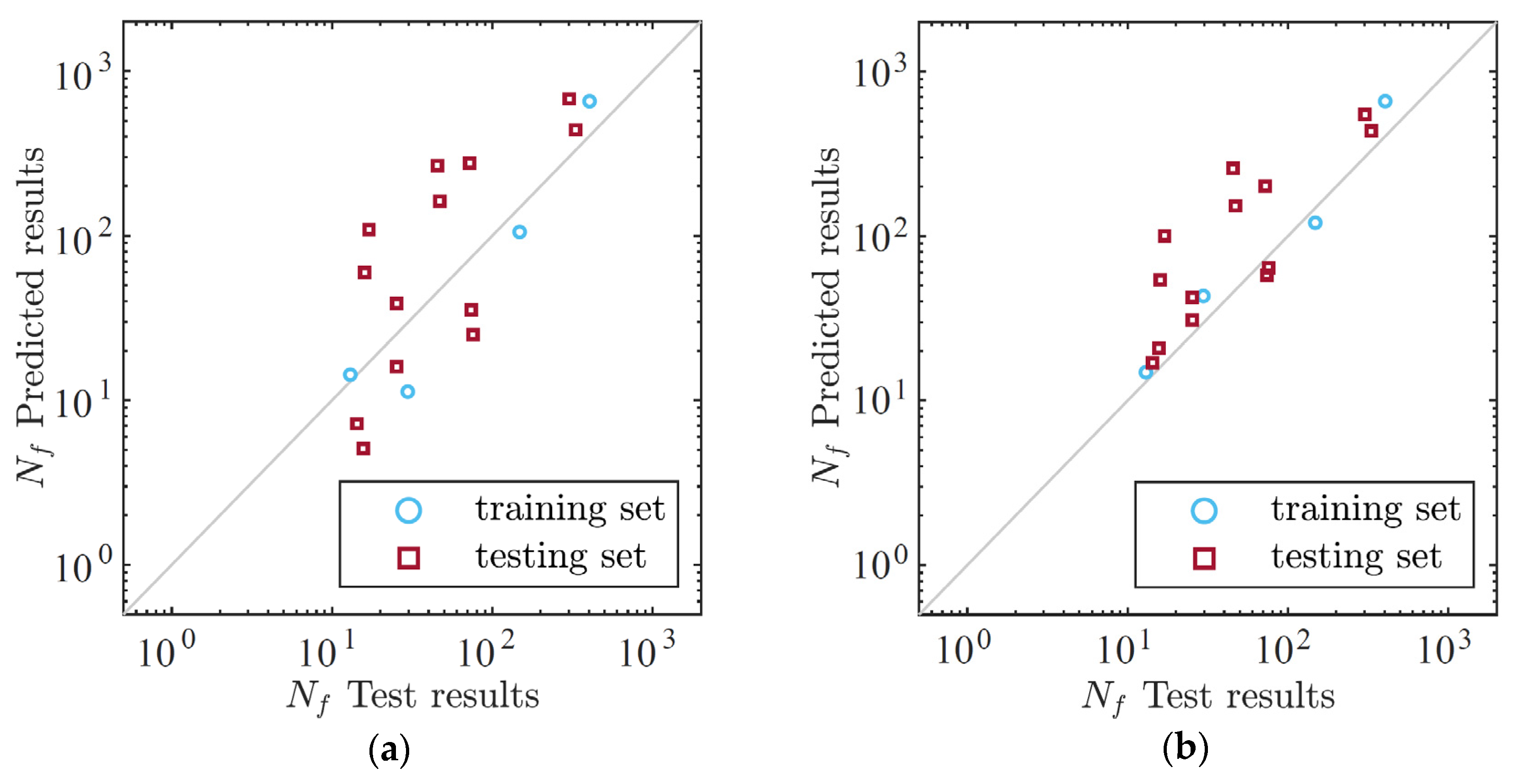
| Baseline model | Training | 0.919 | 253.032 | 163.764 | 0.831 | 365.041 | 214.744 |
| Testing | −0.976 | 144.467 | 99.245 | −0.113 | 108.389 | 74.993 | |
Disclaimer/Publisher’s Note: The statements, opinions and data contained in all publications are solely those of the individual author(s) and contributor(s) and not of MDPI and/or the editor(s). MDPI and/or the editor(s) disclaim responsibility for any injury to people or property resulting from any ideas, methods, instructions or products referred to in the content. |
© 2024 by the authors. Licensee MDPI, Basel, Switzerland. This article is an open access article distributed under the terms and conditions of the Creative Commons Attribution (CC BY) license (https://creativecommons.org/licenses/by/4.0/).
Share and Cite
Xue, X.; Wang, F.; Wang, N.; Hua, J.; Deng, W. Transfer-Learning Prediction Model for Low-Cycle Fatigue Life of Bimetallic Steel Bars. Buildings 2024, 14, 2275. https://doi.org/10.3390/buildings14082275
Xue X, Wang F, Wang N, Hua J, Deng W. Transfer-Learning Prediction Model for Low-Cycle Fatigue Life of Bimetallic Steel Bars. Buildings. 2024; 14(8):2275. https://doi.org/10.3390/buildings14082275
Chicago/Turabian StyleXue, Xuanyi, Fei Wang, Neng Wang, Jianmin Hua, and Wenjie Deng. 2024. "Transfer-Learning Prediction Model for Low-Cycle Fatigue Life of Bimetallic Steel Bars" Buildings 14, no. 8: 2275. https://doi.org/10.3390/buildings14082275