Abstract
This article presents the results of an experimental campaign conducted on a set of four unreinforced masonry walls at full scale. The purpose of this study is to assess, using non-destructive methods, the impact of retrofitting and damage on the modal response of masonry wall systems. Each wall underwent a sequence of increasing cyclic displacements applied by an actuator at the upper end of the specimen. Modal tests based on vibrations were performed both before and after rehabilitation, as well as during the sequence of increasing displacements. It was demonstrated that frequencies can identify progressive damage when the maximum crack is about to occur, as well as the effect of wall retrofitting when mass contribution is considerable. However, the modal assurance criterion indicator (MAC) fails to properly identify a trend of decreasing correlations as progressive damage increases; instead, it is sensitive to detecting maximum crack and instability conditions. Furthermore, it was determined that the coordinated modal assurance criterion indicator (COMAC) does not identify the damage distribution as expected. However, the cumulative COMAC provides a useful tool for quick visualization and interpretation of COMAC behavior. Finally, a novel damage indicator was tested, MACVF, which improves the trend and successfully identifies the most damage-sensitive mode, especially when the maximum level of damage is reached, giving MAC values below 80%. In addition, frequency variations ranged from 70% to 110% when TRM and WWM retrofitting techniques were applied.
1. Introduction
Masonry is a construction technique that combines the use of bricks and mortar, resulting in a heterogeneous material whose properties depend not only on its components but also on its construction process. This construction technique is one of the most widely used worldwide since the materials that compose it are readily available, simple to manufacture, and easy to store, giving it a clear advantage over other modern construction techniques. However, the introduction of reinforced concrete and steel as key construction materials in the 20th century has relegated the study of masonry structures to a secondary position. Consequently, modern structural designers generally have a limited understanding of the mechanical behavior and structural performance of masonry construction [1]. For example, according to the 2017 Census [2], approximately 45% of the national building stock in Chile classifies as masonry constructions and it is especially prevalent in social housing projects financed by the government. Even though this important prevalence exists, dynamic analysis is rarely performed to seismically design masonry buildings because the Chilean standard [3] allows a static equivalent approach for designing buildings of no more than five stories high and less than 20 m high. Therefore, knowledge in Chile of the dynamic behavior of masonry under seismic actions is still limited. This makes masonry construction more vulnerable to seismic events because, in the case of new buildings, the structural design may overlook some particular dynamic behavior that produces local or generalized damage and, in the case of existing buildings, the implemented retrofitting techniques may be ineffective.
In this context, the most affected structures by the seismic events that have occurred in Chile in the last 40 years were masonry buildings. In addition, many of these buildings also presented modifications without complying with technical standards which increased their seismic vulnerability. Astroza et al. [4] reported that the 1985 Algarrobo earthquake (Chile, Mw 7.8) was especially severe for masonry dwellings with three to four stories. More recently, Alcaíno et al. [5] assessed damage in 162 buildings affected by the 2010 Maule earthquake (Chile, Mw 8.8) and found that buildings up to five stories constructed in reinforced or confined masonry presented mild to severe damage and even collapse. Similarly, Núñez Cortez [6] evaluated 110 buildings between four and five stories in the city of Rancagua affected by the 2010 Maule earthquake and revealed that 94% of the masonry buildings evaluated suffered severe damage.
From the point of view of the social and economic impact, significant research has been performed in Chile in order to improve infrastructure and reduce structural vulnerability; however, more research is needed, especially to protect social housing projects. Buildings of this kind might individually represent a relatively small economic value, but collectively, they are one of the most significant components of building stock. Thus, the economic and social impact when they are damaged by an earthquake is immense.
This situation is not only limited to Chile. Ingham and Griffth [7] studied the seismic vulnerability of unreinforced masonry structures in earthquake-prone countries such as Italy and New Zealand. For example, in New Zealand, they reported significant damage in one- and two-story buildings due to the 2011 Canterbury earthquake (Mw 7.1). Most of these are buildings that were constructed prior to the introduction of modern seismic loading standards, and they are characterized by poor seismic performance. Similarly, Habieb et al. [8] reported that buildings up to two stories are not required to submit a structural design in Indonesia and existing building handbooks have only general recommendations to guide this kind of construction. Thus, because of the 2021 Malang earthquake (Mw 6.0), damage ranging from severe to structural collapse was observed in one- and two-story masonry buildings.
This inherent vulnerability of masonry structures added to the age and environmental degradation and the accumulated damage due to precedent seismic events have raised, among communities and local authorities, the concern about the seismic safety of these buildings and have triggered many studies to develop new retrofitting and repairing techniques. For example, Santa María et al. [9], Ozkaynak et al. [10], and Karadogan et al. [11] evaluated the structural performance of carbon fiber-reinforced polymer strips adhered by epoxy resin to masonry panels. Similarly, studies by Griffth et al. [12] and Turkmen et al. [13] evaluated the effect of deep or near-surface mounting strips of CFRP in the strength and ductility of masonry walls. In turn, research by Koutas et al. [14], Gulinelli et al. [15], and Torres et al. [16] evaluated the performance of textile mesh covered by a layer of mortar applied to masonry walls, a technique known as Textile-Reinforced Mortar. Finally, San Bartolomé et al. [17] and Padalu et al. [18] have evaluated a very common technique applied in developing countries, consisting of attaching an electro-welded wire mesh to the masonry panels and covering with shotcrete.
The above experimental studies have demonstrated the effectiveness of these rehabilitation techniques through destructive tests, evidencing an increase in the strength and ductility of masonry walls. Currently, these rehabilitation techniques are widely implemented around the world and exist in many handbooks that describe their application procedures. However, the effectiveness of these rehabilitation techniques strongly depends on the quality of workmanship and the optimal adhesion between the reinforcement material and the masonry wall. This raised the need to develop non-destructive in situ techniques to evaluate the effectiveness of the repair and the improvement in the structural performance of walls.
Several methods for damage detection and structural monitoring based on vibrations have been proposed and implemented. Essentially, these methods aim to assess any significant changes in the dynamic properties of the structure, such as natural frequencies, modal shapes, or damping. Among these techniques, frequency-based methods [19,20,21,22] are the most common and easy to implement since frequency measurements can be quickly obtained. However, damage indicators based on frequencies usually do not provide reliable information about the spatial distribution of damage. Conversely, damage indicators based on mode shapes [23,24,25] could provide information for damage detection, as well as for damage distribution and localization. However, obtaining accurate results requires many measurement points.
Recent laboratory research has conducted damage assessments based on non-destructive techniques, implementing damage identification methods based on frequencies, mode shape, and mode shape curvature [26,27,28,29,30,31]. Among these studies, Oyarzo-Vera et al. [32] evaluated the damage produced by a controlled dynamic load in a scale masonry house. For the identification of damage, they performed low-intensity impact modal tests. They concluded that the degradation of modal frequencies and the modal assurance criterion (MAC) are capable to identify damage, but in some cases these indicators were not efficient in differentiating damage progression. In another study, Oyarzo-Vera et al. [33] evaluated the effect of controlled damage in the modal response of a masonry panel. In that study, damage was applied by cutting a diagonal gap in the panel whose length increases progressively. Although it was possible to detect changes in modal property indicators (frequency and MAC), it was difficult to find a clear trend associated with the loss of stiffness. More recently, Lubrano Lobianco et al. [34] succeeded in evaluating damage in masonry-infilled RC frames by means of modal tests. The analysis of the modal properties allowed us to effectively correlate the degradation in modal frequencies with observable damage in the RC frame masonry infill.
The study presented here evaluates the variation in stiffness in unreinforced masonry (URM) walls due to the implementation of different retrofitting techniques and the induction of damage by applying an in situ non-destructive structural assessment method based on vibrations. This article describes an experimental campaign in which four full-scale unreinforced masonry walls were constructed and tested in laboratory. These walls were retrofitted by applying externally bonded CFRP (EB-CFRP), near-surface-mounted CFRP (NSM-CFRP), textile-reinforced mortar (TRM), and welded wire mesh (WWM) techniques. Subsequently, reversible horizontal loads controlled by a displacement protocol were applied at the top the walls to induce damage. During the cyclic tests, non-destructive modal tests were performed at different states of damage. In these tests, hammer impacts were used to excite the specimen and the vibration response was recorded by a grid of accelerometers. Finally, the modal properties of the structure were identified using system identification techniques. The variations in modal frequencies and modal shapes were analyzed to determine if they could be used as indicators of damage.
Our interest is focused on characterizing the dynamic response of unreinforced masonry structures under elastic conditions and the effect of retrofitting on their dynamic response. This approach aims to create tools that can be applied in the assessment of existing structures and to evaluate the effectiveness of retrofitting strategies.
2. Materials and Methods
2.1. Description of Specimens
Four full-scale URM walls were constructed in the laboratory with dimensions of 1800 (mm) high, 2400 (mm) long, and 145 (mm) thick. The specimens were built with solid clay bricks bonded with a commercially available pre-dosed mortar. The water/mortar mix ratio used was 3.7 (L)/25 (kg) and 20% in mass of the dry mortar was replaced with fine sand to decrease the mix bonding capacity, trying to replicate the conditions of early 20th century masonry in Chile. Masonry prisms were tested following the procedure specified by NCh167 [35]; the results of these material tests are presented in Table 1. In addition, the specimens were built on reinforced concrete foundations, which provided fixed-support conditions at the base (see Figure 1).

Table 1.
Mechanical properties of masonry prisms.
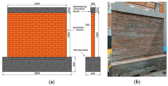
Figure 1.
Specimens: (a) schematic dimension and (b) constructed sample.
During the preparation of the specimens, rehabilitation techniques were applied. The first specimen, designated M2A, was retrofitted using SikaWrap-300c carbon-fiber polymer (CFRP) strips. These strips were externally bonded using Sikadur-300 epoxy resin for impregnation. The fiber strips were cut to a width of 25 cm and arranged in an “X” shape on one side only (see Figure 2a). This technique is known as externally bonded CFRP (EB-CFRP). The second specimen, designated M2B, was retrofitted using a technique known as near-surface-mounted CFRP (NSM CFRP). Carbon fiber cords were embedded near the surface and bonded using a Sikadur-300 epoxy resin for impregnation. These cords had a cross-section of 28 (mm2) and were arranged vertically at an equidistant distance of 60 (cm) between strips and 30 (cm) from the edge (see Figure 2b). Table 2 shows the technical specifications of the materials used in the reinforcements.
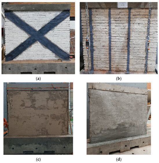
Figure 2.
Wall specimens retrofitted: (a) M2A with EB CFRP, (b) M2B with NSM CFRP, (c) M2C with TRM, and (d) M2D with WWM.
Table 2.
Mechanical properties of CFRP and NSM CFRP materials.
The third specimen, designated M2C, was retrofitted using a technique known as textile-reinforced mortar (TRM). A single-sided carbon fiber textile mesh was installed, bonded by layers of a special anti-seismic mortar called GeoCalce F from KeraKoll. This mesh was arranged in two horizontal sections with an overlap of 15 (cm) (see Figure 2c). Table 3 shows the technical specifications of the material used in the reinforcements. The fourth specimen, designated M2D, was retrofitted using technique known as welded wire mesh (WWM), that utilized a commercially available electro-welded mesh type C-92 with a mesh size of 150 × 150 (mm) and mechanical characteristics of yield and ultimate strength of fy = 641 (MPa) and fu = 675 (MPa), respectively. The mesh covered only one side of the wall and was adhered by layers of manually sprayed stucco (see Figure 2d). For the stucco mixture, a water/cement/sand dosage of 1:2.5:4 was used, from which samples with an average strength of 43.3 (MPa) were obtained.
Table 3.
Mechanical properties of TRM materials.
2.2. Experimental Test and Instrumental Setup
The experimental tests consisted of the application of a quasi-static horizontal cyclic load at the top of the wall. The load cycles are controlled by displacements and follow a sequence that increase its amplitude every three cycles [36], as presented in Figure 3. Horizontal load cycles are applied using a hydraulic actuator and a vertical load was applied using steel chains to prevent wall overturning. Horizontal and vertical loads were recorded during the entire test using load cells and dynamometers. It is important to remark that the cycles defined in the loading sequence in Figure 3 were not executed accurately because the actuator control was performed manually. Therefore, there were small variations in the real maximum displacement reached.
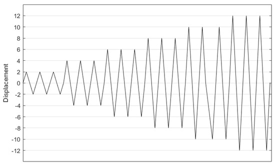
Figure 3.
Cyclic displacement-controlled test protocol.
Each set of three cycles defines a damage state (DS) and an impact modal test is performed for each DS. During these test, horizontal load was released, and a 2 (T) constant vertical load was applied at the top of the wall by testing the vertical chains. The modal test consisted of hammer impact to the wall on a predefined 6-point grid (G1 to G6 in Figure 4), the vibration response of which was recorded by a grid of 12 accelerometers (A1 to A12 in Figure 4), repeating twice the sequence of 6 impacts in the grid points, completing a total of 12 blows in a time of 240 (s) for each modal test. This modal test was executed three times for each DS to verify the repeatability of the vibration response.
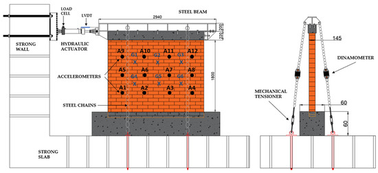
Figure 4.
Experimental set-up.
For the application of the horizontal cyclic load, a steel beam was placed at the top of the walls and fixed to the reinforced concrete top beam by anchor bolts. The ends of the steel beam were mechanically clamped to the upper concrete beam. One end of the steel beam was connected to a 25 (T) hydraulic actuator and a vertical load was applied using steel chains and mechanical tensioners that connected the steel beam to the strong floor, as presented in Figure 4.
The horizontal load was recorded by load cell located at one end of the actuator, measuring load increments in both directions. Similarly, a 150 (mm) stroke LVDT was used to measure the horizontal displacements. These sensors were located horizontally and parallel to the actuator. To complete the data acquisition system, the load and deformation sensors were connected to NI 9237 and NI 9205 modules mounted on a NI cDAQ-9174 chassis and to a laptop that allowed real-time control and digitization of the data using a routine implemented in LabView software.
In the case of modal tests, the instrumental setup consisted of a grid of 12 accelerometers; 8 of them are uniaxial accelerometers model 352C03 and 4 uniaxial accelerometers are model 333B50, both from PCB Piezotronics. These were fixed to the specimen wall using screws. The accelerometers were connected by shielded cables to NI 9234 data acquisition modules, mounted in a NI cDAQ9174 chassis. The data were digitized through a routine implemented in LabView software, and a sampling rate of 1652 samples per second was used.
2.3. Damage Indicators
The vibration response recorded by the accelerometers due to impacts were analyzed using operational modal analysis techniques, assisted by the software Artemis Modal Pro v6.0. The frequency range was reduced by decimating the time series to the interval 0 to 41.3 Hz, which is the range of interest of our experiments. Also, an eighth-order Chebyshev Type 1 low-pass filter was applied to the signal. The modal identification was carried out using two methods: Enhanced Frequency Domain Decomposition (EFDD) and Stochastic Subspace Identification (SSI-UPC). For the EFDD method, a manual selection of modal frequency peaks was performed, verifying immediately in the geometry window the modal shape associated with the frequency. And for the SSI-UPC method, the software performed an automatic estimation of modes. In both methods, only modes with a damping not greater than 15% were considered. For each damage state (DS), three modes were identified, recording the average modal frequency () and mode shape vectors () extracted from the results of the 12 hits performed at each impact point.
Damage indicators were employed to explore the correlation between retrofit interventions or induced damage with the observed changes in the modal properties of the walls. The first damage indicator considered in this study was the variation in the walls’ modal frequencies at different stages of damage. This indicator has been widely used in several studies [19,20,21,22,23,28] because of its intuitive predictability that helps analysts to validate results in a rapid manner. However, these studies have also demonstrated that this indicator is not always effective in detecting damage at early stages.
Another set of damage indicators considered in this investigation was based on changes in the mode shape due to retrofit interventions or damage. The first mode shape damage indicator considered in this study was the modal assurance criterion (MAC), representing the squared linear regression correlation coefficient, providing a measure of coherence between two compared vectors. Based on this analysis, modal vectors were compared for two different experimental states ( in Equation (1)). The resulting values of the MAC range between 0 and 1, representing totally uncorrelated and highly correlated modes, respectively. It is worth noting that the MAC is sensitive to significant differences between corresponding components of the compared vectors, but it is essentially insensitive to small changes and small magnitudes of modal displacements.
The second damage indicator considered to assess the correlation of pairs of mode shape vectors is the normalized modal difference (NMD). This damage indicator represents a close estimate of the average difference between the components of two vectors and is more sensitive to differences between pairs of modes than the MAC. Therefore, it allows for the observation of differences between highly correlated modal shapes. The calculation of this indicator was performed using Equation (2). An NMD value close to 0 indicates a high correlation between the modes.
The modal assurance criterion of coordinates (COMAC) was considered as a third indicator based on mode shapes. This indicator reveals the spatial distribution of the degree of correlation and retains information about individual degrees of freedom. It was calculated using Equation (3), where “r” denotes the r-th component of the k-th mode shape in experimental state 1 and 2. A low COMAC value indicates poor correlation in the corresponding degree of freedom.
Derived from the MAC, a novel indicator is introduced in this study, MACVF. This indicator incorporates the contribution of frequency variation between two pairs of states of the same frequency. Equation (4) defines this new indicator.
The parameter described by corresponds to the variation in the relative frequency between two states e1 and e2 for the k-th mode and is obtained from Equation (5). This is entered in terms of a ratio in Equation (4).
3. Results
3.1. Cyclic Test Results
The four specimens were tested following the cyclic loading sequence presented in Figure 3. Figure 5, Figure 6, Figure 7 and Figure 8 show the wall conditions before and after testing.
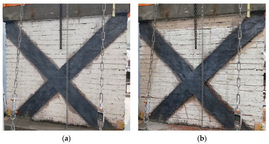
Figure 5.
Specimen M2A (a) before test (b) after test.
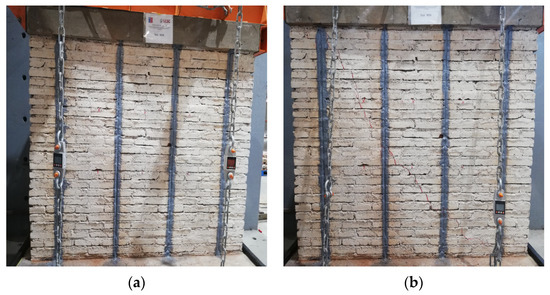
Figure 6.
Specimen M2B (a) before test (b) after test.
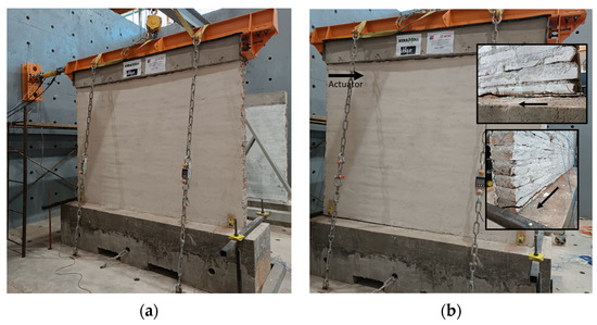
Figure 7.
Specimen M2C (a) before test (b) after test.

Figure 8.
Specimen M2D (a) before test (b) after test.
For wall M2A, the first crack was observed at the base, between the first and fifth rows of bricks in the wall. This crack occurred during the 8 mm cycle, reaching a maximum displacement of 10.4 mm with a load of 57.6 kN. At the 10 mm cycle, the CFRP strip began to detach from the wall in the area near the crack, reaching 11.7 mm of maximum displacement and 59.3 kN. In subsequent loading cycles, the width of the crack increased, and new fractures were detected near the CFRP reinforcement band in the direction of its diagonals but mainly in the lower area of the wall. As the displacements increased, the reinforcing bands progressively began to peel off until they completely detached from the surface by adhesion. Total failure of the wall occurred during the 18 mm cycle, reaching a maximum displacement of 17.3 mm and a load of 79.6 kN.
For wall M2B, the first sign of a crack was observed at the base of the wall. This crack occurred during the 6 mm cycle, reaching a maximum displacement of 7.7 mm with a load of 30.6 kN. In subsequent cycles, the wall did not show an increase in cracks and behaved elastically without detachment of the CFRP cords, completing the 18 mm cycle. Subsequent displacements were applied using a monotonous cycle, progressively increasing every 2 mm. At 26 mm the panel showed the first symptoms of diagonal cracking; however, the final failure only showed when a displacement of 29 mm and a load of 91.2 kN were reached. This failure was brittle. Finally, the CFRP cords embedded in the wall were cut in the area where the crack occurred.
Comparing both walls, it is observed that both walls experience an initial failure at the base at similar levels of displacements (M2A at 10.4 mm and M2B at 7.7 mm). However, the fault in wall M2A propagates following a stepped pattern between the first and fifth rows of bricks, while wall M2B experiences an adherence failure at the base of the wall in a single line. In subsequent cycles, wall M2A experienced crack growth and detachment of the CFRP strips mainly in the lower diagonals. In contrast, the M2B wall had an elastic behavior in the panel during the subsequent cycles up to 18 mm, maintaining a localized failure propagation at the base. Finally, both walls reached their collapse, but wall M2B managed to achieve greater deformation and load than M2A.
For wall M2C, the first crack was observed at the base of the wall during the 6 mm cycle, reaching a maximum displacement of 6.8 mm with a load of 31.6 kN. In subsequent loading cycles, no new cracks were observed, and the damage consisted solely of an increase in failure at the mortar joint at the base. The test was completed by finishing the 26 mm cycle, reaching 27.2 mm displacement and a load of 79.5 kN.
For wall M2D, the first sign of a crack was also observed at the base of the wall during the 6 mm cycle, reaching a maximum displacement of 6 mm with a load of 23.58 kN. In subsequent loading cycles, no new cracks were observed, and the damage consisted solely of an increase in failure at the mortar joint at the base. The test was completed by a cycle that reached a displacement of 26.7 mm and a load of 86.3 kN.
Figure 9 shows the maximum values of the extension and contraction branches of the cyclic tests. In the extension zone, the M2A wall presents the steepest slope in both the extension and contraction branches, indicating that this retrofitting with EB-CFRP bands provides greater stiffness against lateral loads. Walls M2B and M2C show similar stiffness in extension branch. However, M2B reaches a final brittle failure at 29 mm with 91.2 kN and the M2C wall shows elastic behavior in the wall and only concentrates the failure at its base, ending the test at 27.2 mm and 79.5 kN. With respect to the contraction branch, it is observed that the M2C wall has a stepper slope than the M2B wall, demonstrating that the wall retrofitted with TRM gives it greater stiffness. It is important to note that this behavior in the contraction branch was not possible to analyze during the subsequent cycles because, due to limitations of the instruments and actuator, both walls were subjected to extension cycles only from the 16 mm cycle onwards.
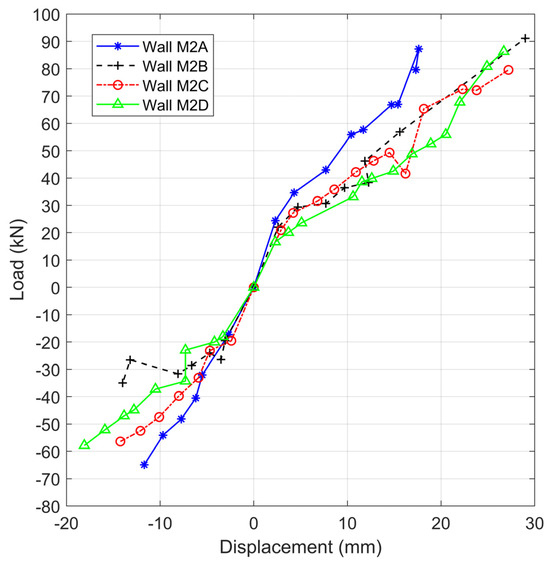
Figure 9.
Maximum displacements from cyclic tests.
Regarding the behavior of walls M2C and M2D, it is crucial to note that the slopes of these curves are not only generated by the elastic deformation of the wall but also by the rocking at the base. Therefore, the slope of these curves does not represent the stiffness of the masonry panel and the rocking effect must be considered. This effect is produced by the early adherence failure experienced at the base of the wall, which progressively increased as the displacements increased. It should also be noted that the M2C wall suffered an out-of-plane misalignment when the 14 mm cycle was executed in the extension branch. It is possible to observe that both walls present a similar behavior in the extension branch. In contrast, in the contraction branch it is observed that the wall M2D reinforced with the WWM technique has a smaller stiffness than the wall M2C reinforced with the TRM technique. Again, both walls were subjected only up to the 16 mm cycle in contraction due to equipment limitations.
Finally, it is important to note that the adherence failure in walls M2C and M2D causes the displacements induced in the upper part of the wall to concentrate the damage only at the base. This leads to both walls mostly experiencing an elastic behavior of the panel, and they were mainly affected by an out-of-plane failure because of the misalignment of the wall when the panels detach from the base at maximum displacement.
3.2. Damage Identification Results
The modal tests conducted on the walls obtained the modal frequencies corresponding to undamaged states, with retrofitting, and after each cyclic test performed on the wall. Table 4 presents the frequencies f1, f2, and f3 obtained for the undamaged state of M2A, M2B, M2C, and M2D. It is observed that the frequencies are similar for the four walls, which were constructed with the same dimensions and mechanical properties.
Table 4.
Modal frequencies (Hz) in non-retrofitted condition.
The modal shapes for the walls M2A, M2B, M2C, and M2D are presented in Figure 10. These correspond to the initial undamaged state in their first three modes associated with frequencies f1, f2, and f3. It is worth noting that the obtained modal shapes remain similar across the four walls for the undamaged state, where the first mode represents translational displacement (see Figure 10a), the second mode represents torsional rotation (see Figure 10b), and the third mode represents flexural bending (see Figure 10c).
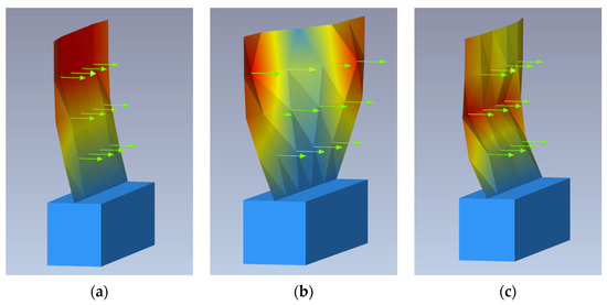
Figure 10.
Reference images of the experimental mode shapes for (a) mode 1, (b) mode 2, and (c) mode 3.
The relative variations in frequencies due to retrofitting are graphically depicted in Figure 11. The frequency values presented there correspond to the average result of six data points for a particular frequency obtained through the EFDD and SSI modal identification methods. The blue color of the bars represents the non-retrofitted states, while the yellow color indicates the retrofitted states.
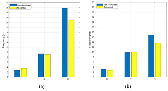
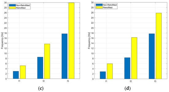
Figure 11.
Variation in frequencies due to retrofitting effects: (a) M2A, (b) M2B, (c) M2C, and (d) M2D.
In Figure 11a, a slightly significant increase in frequency f1 is observed, while in Figure 11b, a slightly significant decrease is noted. This occurs similarly for frequency f3 of walls M2A and M2B, which show an unexpected decrease of 17% and 19%, respectively, after retrofitting was implemented. On the other hand, in Figure 11c,d, the significant effect of WWM and TRM reinforcement techniques is evident. The behavior of the bars shows a clear increasing trend in frequencies f1, f2, and f3, where frequency f1 increased by up to 73% and 108% for walls M2C and M2D, respectively. Therefore, frequencies are unable to detect changes when retrofitting that does not significantly increase mass in the structures is applied.
Figure 12, Figure 13, Figure 14 and Figure 15 depict the frequency variability in the data sets for walls M2A, M2B, M2C, and M2D, respectively. The index DSi indicates a damage state associated with the displacement i reached during the loading cycle. In these plots, the length of the box and its bounds, known as upper and lower whiskers, indicate the variability in the data obtained from measurements for the same damage state, allowing for a quick visual check to infer whether frequency variations between two compared states could be influenced by inherent measurement errors rather than induced damage. Additionally, the value of the medians is represented by a horizontal red line inside the boxes, and comparison intervals are limited by the centers of the upper and lower triangular markers. These intervals allow determining whether two medians are significantly different with a confidence level of 95%.
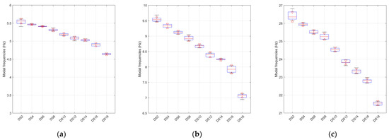
Figure 12.
Modal frequencies variation for wall M2A: (a) f1, (b) f2, and (c) f3.
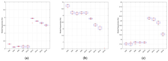
Figure 13.
Modal frequencies variation for wall M2B: (a) f1, (b) f2, and (c) f3.
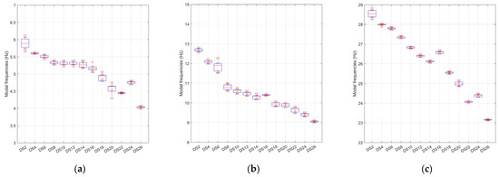
Figure 14.
Modal frequencies variation for wall M2C: (a) f1, (b) f2, and (c) f3.
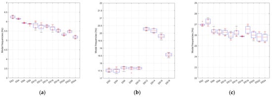
Figure 15.
Modal frequencies variation for wall M2D: (a) f1, (b) f2, and (c) f3.
Figure 12a–c show the data set plots for wall M2A associated with frequencies f1, f2, and f3, respectively. In this figure, there is a clear trend of decreasing median frequencies as the displacements of the test cycle increase. Additionally, it is observed that the limits of the data set, represented by their whiskers, generally do not overlap between one state and its consecutive one. For example, for frequency f2, between the medians of states DS4 and DS6 or DS16 and DS18, they are significantly different with a confidence level of 95%.
Figure 13a–c depict the data set plots for wall M2B associated with frequencies f1, f2, and f3, respectively. In this figure, there is no clear trend in the variation in median frequencies as the displacements of the test cycle increase. For example, it is noted that the limits represented by the whiskers of the data sets for states DS6, DS8, and DS10 of frequencies f1 and f3 overlap, indicating that the variation in frequencies is due to data acquisition variation. Additionally, for f1, f2, and f3, it can only be affirmed that the means are significantly different with a confidence level of 95% from state DS14 onwards.
Figure 14a–c display the data set plots for wall M2C associated with frequencies f1, f2, and f3, respectively. Although there is a clear trend of decreasing median frequencies as displacements increase, when comparing the data sets of two consecutive states, their whiskers may overlap, indicating that the variability may be associated with data variation rather than damage. This relative variation between frequencies could be confirmed by comparing the data set with a reference state such as DS2. For example, for f2, the DS2 data set does not overlap with the data sets of successive states, confirming that the means of the compared states are significantly different and, therefore, the relative frequency variation with respect to DS2 is associated with damage rather than data variation.
Figure 15a–c show the data set plots for wall M2D associated with frequencies f1, f2, and f3, respectively. Similar to Figure 14, consecutive medians do not show a clear decreasing trend. For example, it is observed that for f1, the data sets between two consecutive states overlap. Once again, to establish that two medians are significantly different, it is necessary to compare two non-consecutive states, that is, maintain an initial reference state.
Figure 16 and Figure 17 represent the relative variations in frequencies f1, f2, and f3 for walls M2A, M2B, M2C, and M2D.
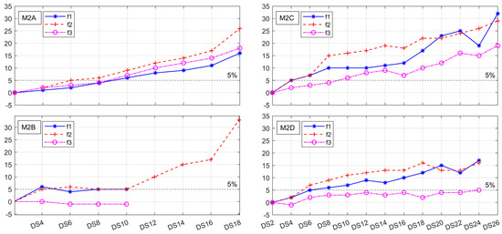
Figure 16.
Frequency variation calculated using DS2 damage state as reference.
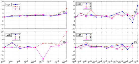
Figure 17.
Frequency variation between the damage states and their successive DSs.
Figure 16 shows the relative frequency variations between the initial state DS2, taken as a reference, and another state DS. The x-axis indicates the index of the compared damage state; for example, state DS4 represents the difference between DS2 and DS4. Similarly, state DS6 indicates the relationship between DS2 and DS6 and so on. For wall M2A, there is a clear trend of over 5% relative decrease in frequency for f1, f2, and f3. In the case of wall M2B, only frequency f2 detects decrements greater than 5% in the frequencies, while f1 and f3 showed an unexpected increment in frequencies starting from the DS10 state. This is associated with noise detected on the second day of testing and, consequently, a poor identification of the peak in the modal processing. Therefore, these measurement points are not considered in the analysis. Similarly, walls M2C and M2D show a trend of increasing relative decrease in their frequencies. Additionally, across all four walls, frequency f2 exhibits the best sensitivity to variations due to induced damage.
On the other hand, Figure 17 depicts frequency variations between two consecutive states. The x-axis indicates the index of the subsequent state; for instance, state DS4 represents the difference between DS2 and DS4. Similarly, state DS6 indicates the relationship between state DS4 and DS6 and so forth. For wall M2A, it is shown that relative frequency decreases of over 5% occur after reaching 18 mm of displacement, at which point the wall fails. In the case of wall M2B, similar decrements in relative frequency variations of more than 5% are observed once 18 mm is reached, at which point the wall exhibited signs of cracking near the retrofitting cables. However, f1 showed an unexpected increment in frequencies starting from the DS10 state, and this is associated with noise detected on the second day of testing and, consequently, a poor peak identification in the modal processing. For walls M2C and M2D, only frequency f2 can identify decreases after reaching displacements of 8 mm and 6 mm, respectively, which could be associated with the moment when adhesion failure occurred and a slight deviation from the wall plane.
Figure 16 and Figure 17 allow visualization of the behavior of relative frequency variations using an initial state as reference and comparing two consecutive states. Additionally, it is possible to identify whether there is a trend in the variations or if significant variations are identified when visible damage occurs in the wall, such as cracks in the plane, adhesion failures, and misalignment of the plane.
Figure 18 presents the MAC calculated for each wall considering the mode shapes extracted for the DS2 state as reference, while Figure 19 presents the MAC values calculated for each DS using the mode shape extracted preceding DS as reference (example: DS2 relative to DS4 and DS4 relative to DS6). The values of 1-MAC were plotted in the figures to detect subtle improvements between the two states.
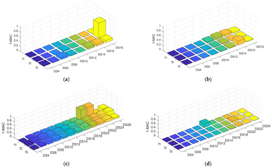
Figure 18.
MAC calculated using DS2 as reference: (a) M2A, (b) M2B, (c) M2C, and (d) M2D.
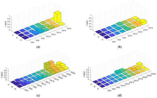
Figure 19.
MAC between consecutive DSs: (a) M2A, (b) M2B, (c) M2C, and (d) M2D.
Figure 18 generally shows a high correlation for modes 1, 2, and 3 in walls M2A, M2B, and M2D. In Figure 18a, it is not possible to identify a decreasing trend in correlations for wall M2A. However, a slight change is observed for mode 3 when it reaches state DS14 compared to reference state DS2. The MAC value decreases to 92% and remains the same until the final state DS18. These variations could be attributed to the first crack at the base of the wall and the appearance of initial symptoms of wall cracks. The greatest decrease in the MAC is shown for mode 2 between states DS2 and DS18 (36%). On the other hand, in Figure 18b, only slight changes are observed in the shape of mode 1 and mode 3 once state DS12 is reached.
In Figure 18c for wall M2C, only mode 2 shows a clear decreasing trend in correlation starting from state DS6. However, the greatest changes are observed from state DS16 onwards, with the decrease in the MAC reaching 80% at state DS26. These decreases do not align with the damage observed on the wall during testing, but they could be associated with increased adhesive failure at the base and deviation from the plane. On the other hand, in Figure 18d for wall M2D, there is no decreasing trend in correlations identifying changes in modal shapes.
Figure 19 in general shows a high correlation for modes 1, 2, and 3 in walls M2A, M2B, and M2D. In Figure 19a for wall M2A, it is not possible to identify a decreasing trend in MAC. However, it is possible to identify a decrease to 63% in MAC for mode 2 when reaching state DS18 compared to mode DS16. On the other hand, in Figure 19b, changes are only observed for mode 3 when reaching state DS16, with an 80% MAC value. In Figure 19c for wall M2C, it is observed that once state DS20 is reached, there is a decrease in mode correlations that persists until state DS26. This variation in modes was not observed as wall cracks during testing. However, they could be associated with adhesive failure at the base and deviation from the plane. On the other hand, in Figure 19d for wall M2D, there is no decreasing trend in correlations identifying changes in mode shapes.
Figure 20 represents the behavior of the NMD index, which compares a mode associated with a DS relative to the initial state DS2. The blue line corresponds to the mode associated with frequency f1, the red line to frequency f2, and the magenta line to frequency f3. In Figure 20a, a good correlation is observed with values close to 0. However, slight changes can be seen for the mode associated with frequency f3 and f2, but these do not show a clear trend as displacements increase. On the other hand, Figure 20b shows variations for modes associated with frequencies f1 and f3, which from state DS10 onwards exhibit a decreasing trend in mode correlations.
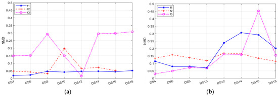
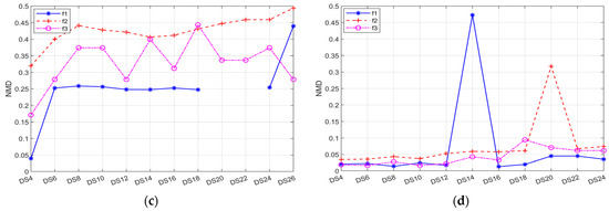
Figure 20.
NMD: (a) M2A, (b) M2B, (c) M2C, and (d) M2D.
In Figure 20c, only the mode associated with frequency f2 allows identifying a decreasing trend in correlations, with an NMD value of 0.5 once state DS26 is reached. On the other hand, in Figure 20d, the correlation between modes is very good, and it is not possible to identify decreases associated with damage at the base of the wall.
Figure 21 presents the 12 degrees of freedom defined for the measurements. On the other hand, Figure 22 presents the COMAC calculated for each wall considering the mode shapes extracted for the DS2 state as reference, while Figure 23 presents the COMAC values calculated for each DS using the preceding mode shape extracted as reference.
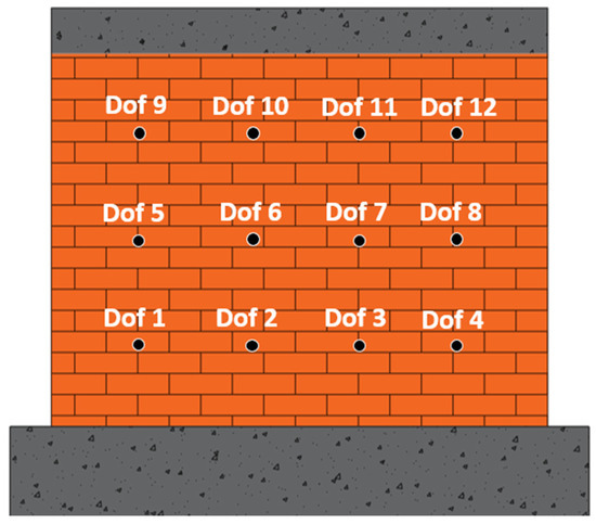
Figure 21.
Degrees of freedom.
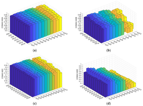
Figure 22.
COMAC calculated using DS2 as reference: (a) M2A, (b) M2B, (c) M2C, and (d) M2D.

Figure 23.
COMAC between consecutive DSs: (a) M2A, (b) M2B, (c) M2C, and (d) M2D.
In Figure 22a, a very high correlation is evident, exceeding 92%. However, decreases are identified in degrees of freedom 9, 11, and 12, which intensify upon reaching state DS16. Similarly, in Figure 22b, greater dispersion is observed in degrees of freedom 5–12, and correlations decrease as displacements increase.
On the other hand, for wall M2C, Figure 22c shows a decrease in correlations for degrees of freedom 9–12, changing up to 85% in degrees of freedom 9 and 12 upon reaching state DS18. Finally, in Figure 22d, although low correlation values are recorded, there is no evidence of a decreasing trend as displacements increase.
In Figure 23a, a very high correlation is observed, also exceeding 92%. However, decreases are identified in degrees of freedom 9 to 12, which intensify upon reaching state DS16. Similarly, in Figure 23b, greater dispersion is observed in degrees of freedom 5–12, and correlations decrease as displacements increase.
On the other hand, for wall M2C, Figure 23c shows a marked reduction in correlations for degrees of freedom 9 and 12. Additionally, changes are identified as displacements increase; for example, degree of freedom 12 experiences a correlation decrease from 92% to 85% upon reaching state DS20, and then further decreases upon reaching state DS26. Finally, in Figure 23d, although low correlation values are recorded, there is no evidence of a decreasing trend as displacements increase.
A clear way to visualize the changes in the COMAC value for each degree of freedom is to calculate the cumulative difference based on the COMAC correlation values for each DOF. This result is graphically represented using bars, with Figure 24 showing the cumulative difference from the COMAC calculated with the DS2 state as reference, and Figure 25 for the COMAC calculated between two consecutive states.

Figure 24.
Accumulated COMAC calculated using DS2 as reference: (a) M2A, (b) M2B, (c) M2C, and (d) M2D.
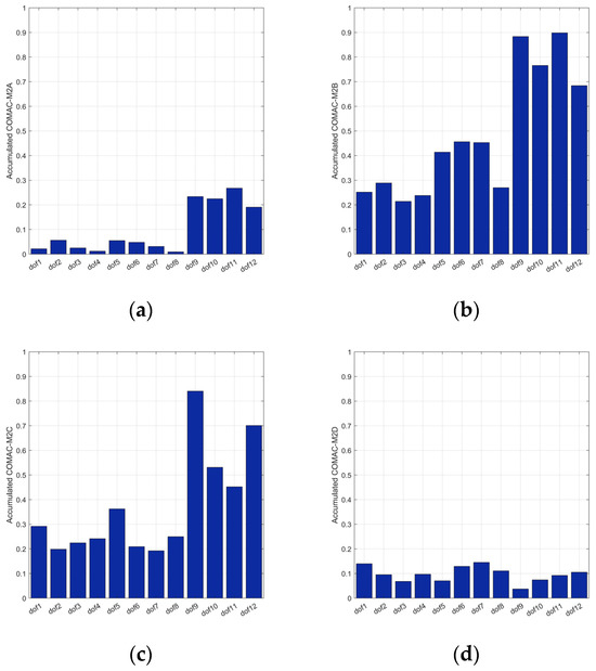
Figure 25.
Accumulated COMAC between consecutive DSs: (a) M2A, (b) M2B, (c) M2C, and (d) M2D.
In Figure 24a, it can be observed that the COMAC calculated for wall M2A shows the greatest decreases in correlation for DOFs 9, 10, 11, and 12. However, the damage experienced during the test occurred near DOFs A1, A2, A3, and A4 (see Figure 4 and Figure 5b). Similarly, for wall M2B, the greatest decreases in correlation are achieved for DOFs 9, 10, 11, and 12. Additionally, it is possible to identify that DOFs 5, 6, and 7 show decreases greater than 0.2 points. However, the damage experienced during the test occurred on the wall’s diagonal, close to DOFs 9, 6, 3, and 4 (see Figure 4 and Figure 6b). Therefore, although the COMAC manages to identify decreases in correlations for each DOF, it failed to identify the spatial distribution of the damage on the wall even though a significant failure occurred.
On the other hand, for wall M2C in Figure 24c, the greatest decreases in correlation are identified for DOFs 9 and 12. However, the damage experienced during the test occurred at the base of the wall, near DOFs 1, 2, 3, and 4. Similarly, for wall M2D in Figure 24d, the COMAC was unable to identify major decreases for the DOFs near the base. Therefore, the COMAC failed to identify the distribution of the damage caused by adhesive failure.
In Figure 25, a similar behavior in the decreases of correlation for each DOF is observed. It is possible to identify that regardless of the reference state used to calculate the COMAC, this indicator fails to identify a clear distribution of the damage experienced on the wall.
Figure 26 presents the MACVF calculated for each wall considering the mode shapes extracted for the DS2 state as reference, while Figure 27 presents the MACVF values calculated for the mode shapes extracted for each DS using the preceding mode shape extracted as reference. Equation (4) and the parameter from Equation (5) were used for the calculation, and the values of 1-MACVF were plotted in the figures to detect subtle improvements between the two states.

Figure 26.
MACVF calculated using DS2 as reference: (a) M2A, (b) M2B, (c) M2C, and (d) M2D.
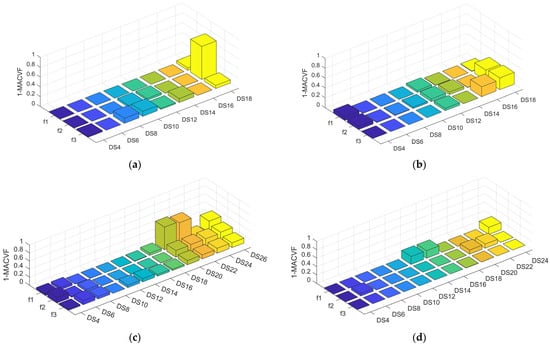
Figure 27.
MACVF between consecutive DSs: (a) M2A, (b) M2B, (c) M2C, and (d) M2D.
In Figure 26a, it is observed that from states DS8 and DS10, the correlations for modes 1, 2, and 3 begin to decrease. It is noted that as displacements increase, the modes start to undergo changes, which could be related to the initial signs of cracks in the wall near the final failure (see Figure 5b). Similarly, in Figure 26b, mode 2 is the only one showing a decreasing trend in correlations, with a drop in the MAC of 66% when reaching state DS18. This decrease makes sense, as the final failure occurred at 29 mm, and when 18 mm were reached, only cracks near the diagonal were observed.
In Figure 26c, it is highlighted that mode 2 is the most sensitive to changes in correlations. It exhibits a more pronounced trend of MAC decrease and could be related to the instability of the wall due to adhesive failure, which caused an out-of-plane inclination and rotation since the actuator kept a fixed point at the top of the wall. In Figure 26d, there is no clear trend of decreasing correlations observed, as the wall did not experience damage and did not undergo a noticeable out-of-plane inclination.
In Figure 27, the proposed MACVF indicator fails to highlight and identify a trend in MAC correlation values. This is because the variations considered significant in Figure 17 are only experienced when a significant failure in the wall occurs. Therefore, the MAC and MACVF cannot identify damage unless cracks or significant wall inclination are observed. On the other hand, the MACVF allows for better highlighting of a trend than the MAC. Additionally, it manages to highlight and thus identify which mode was the most sensitive to changes due to the appearance of cracks or significant inclination and rotation.
Figure 28 shows the average value of (1-MAC) and (1-MACVF) calculated from the three modes for each wall considering the DS2 state as a reference, while Figure 29 considers consecutive DSs. The average value of (1-MAC) and (1-MACVF) range between 0 and 1, where 1 indicates no correlation between the mode shapes and 0 indicates a very good correlation.
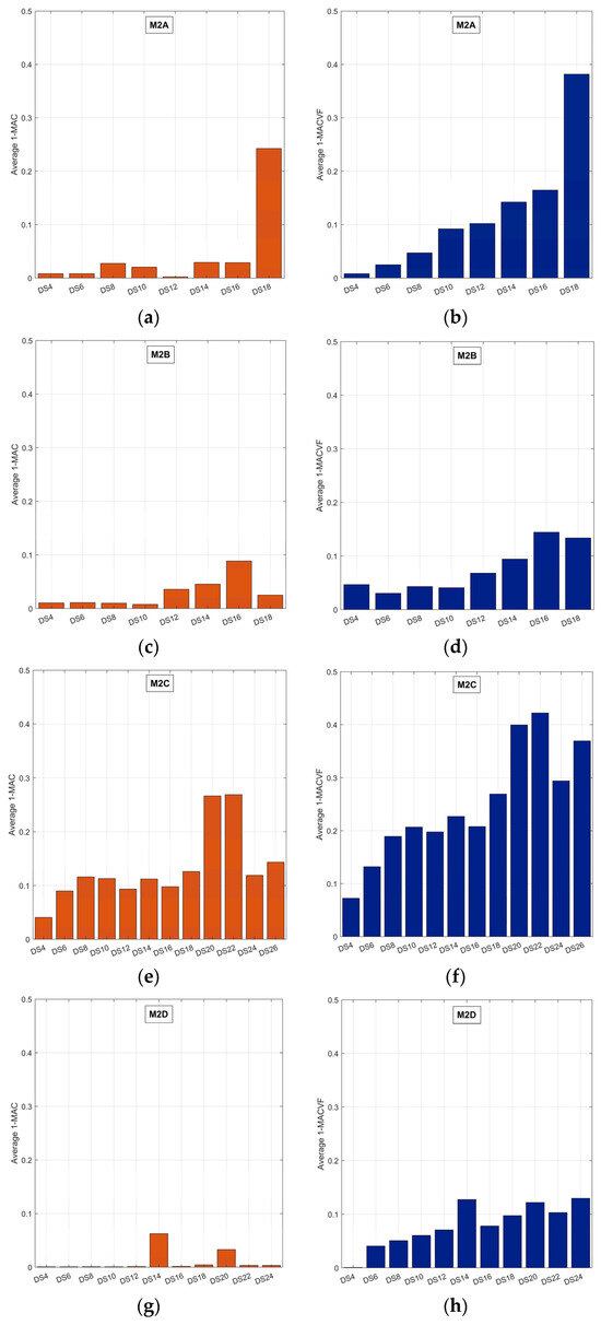
Figure 28.
Average (1-MAC) and Average (1-MAC) calculated using DS2 as reference for (a,b) M2A, (c,d) M2B, (e,f) M2C, and (g,h) M2D.
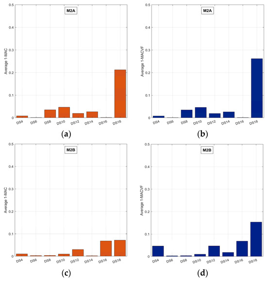
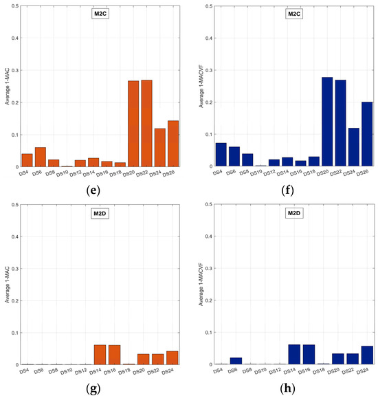
Figure 29.
Average (1-MAC) and Average (1-MAC) calculated using consecutive DSs for (a,b) M2A, (c,d) M2B, (e,f) M2C, and (g,h) M2D.
In Figure 28a, a high correlation of modal shapes in the M2A wall is quickly visualized. Although slight variations are observed, these do not represent a significant increment in Average (1-MAC) and do not exceed 95%. However, a significant change is observed when the wall failure is reached at state DS18. On the other hand, in Figure 28b, an increasing trend in Average (1-MACVF) correlation is evident; however, significant changes occur from state DS14 onwards, where the Average (1-MACVF) shows an increment greater than 90%.
In Figure 28c for wall M2B, a slight trend is observed from state DS12. However, only once state DS16 is reached does the Average (1-MAC) experience an increment close to 90%. Similarly, in Figure 28d, an increment greater than 90% in Average (1-MACVF) is observed once state DS16 is reached, indicating a slightly increasing trend. It is worth noting that the final failure in wall M2B occurs after state DS18, and until that state, only cracks near the reinforcement and at the ends of the failure diagonal were observed.
In Figure 28e for wall M2C, no increasing trend in Average (1-MAC) correlations is observed; however, increments greater than 90% in Average (1-MAC) are seen from state DS18 onwards. Additionally, in Figure 28f, the Average (1-MACVF) highlights an increase greater than 90% but does not show a clear increasing trend in correlations. These non-trending increases do not align with the observed damages but could be associated with wall deviation due to adhesive failure.
Finally, in Figure 28g for wall M2D, no significant increments in Average (1-MAC) value are observed. Similarly, in Figure 28h, although Average (1-MACVF) identifies a slight trend, these increases are generally smaller than 90% and do not align with what was observed in the wall during testing.
In Figure 29, when comparing the Average (1-MAC) with Average (1-MACVF) between consecutive damage states, no significant changes are observed. This is because the variations considered significant (10%) are only experienced when a major failure occurs in the wall.
4. Discussion
Complementary to the results presented in the precedent section, it is worth making a comment regarding to the reliability of the system identification procedures employed to determine the modal properties of the walls. Both system identification methods (EFDD and SSI) have been widely used in several studies to determine the modal properties of URM structures [19,20,21,26]. Nevertheless, several verifications were performed in this study to determine the reputability and replicability of these experiments and to check the reliability of the obtained modal data. In the case of modal frequencies, it was verified that the Coefficient of Variation (CoV) of the same frequency detected by different methods and in different test were always smaller than 5%. While, in the case of the mode shapes, they were tested bay calculating the MAC between pairs of vectors obtained by different methods and in different tests. In all these cases, the MAC was larger than 98% for modal vectors associated with the same mode, demonstrating the repeatability of the detected mode shapes. When these conditions were not satisfied, this set of data was discarded. In the entire experimental procedure, 161 of 918 sets of data were discarded.
Regarding to the use of modal frequencies as damage indicators, the obtained frequencies before and after retrofitting were able to detect the structural intervention showing significant increases in frequencies. However, these increases occurred only when a retrofitting technique was widespread in the entire face of the wall and significantly increased the mass and stiffness of the system (walls M2C and M2D). In the case of “lighter” structural interventions, such as the use of CFRP strips and cords (walls M2A and M2b), no significant changes are observed.
Similarly, the frequencies showed sensitivity to deteriorations due to progressive damage. A fairly linear decay was observed, even when cracks were not visible in walls M2A and M2B (see Figure 12, Figure 13 and Figure 16). The greatest decreases were recorded when the maximum crack condition (walls M2A and M2B) and/or maximum wall instability (walls M2C and M2D) were reached. Additionally, the frequencies were consistent with visually observed changes, identifying slight variations or maintaining a flat trend for wall M2D (see Figure 15 and Figure 16), which only had a base flaw causing a slight inclination compared to its counterpart, wall M2C.
Lastly, the frequencies failed to identify base faults like those experienced in walls M2C and M2D, as when the wall returned to its original position, this crack became imperceptible. Instead, the frequencies identified changes if the adhesion fault led to an inclination due to wall instability when reaching a maximum condition, as occurred in wall M2C.
This good correlation between damage progression and modal frequency decrement was expected and has been reported before [26,27,32,33]. In general, modal frequencies are parameters that are precisely measured; hence, the test repeatability and replicability is easy to guarantee, as in this case where the CoVs of the modal frequencies are smaller than 5% (2% on average). That makes modal frequency degradation a reliable damage indicator. However, when damage is localized as in the case of walls M2C and M2D, and the specimen kinematics was already affected by this localized damage, modal frequency degradation may not be sufficient to detect further damage because it tends to stabilize.
The MAC damage indicator, based on modal shapes, generally identified a high correlation for modes 1, 2, and 3 during the damage states reached due to progressive imposed damage. This indicator only detected significant decreases in correlations when a maximum crack or instability condition, caused by base opening, was reached. It was expected that the MAC indicator would be able to detect decreases and show a trend even when cracks were not observed or when the first symptoms appeared.
The NMD indicator, based on modal shapes, generally did not improve the results of the MAC, identifying a trend for the three modes. However, for wall M2B (see Figure 20), it identified a better trend for modes 1 and 3. The values determined by NMD generally did not exceed 0.45 points, indicating that the MAC showed a decrease in its maximum condition by 80%.
The COMAC indicator, based on modal shapes, determined high correlations for degrees of freedom. It was expected that this indicator could identify a decreasing trend and a precise damage distribution. However, the greatest variations were identified for degrees of freedom 9, 10, 11, and 12, corresponding to the four upper degrees of freedom (see Figure 4). For example, it was expected to identify a greater decrease in correlations for degrees of freedom near the cracks experienced in walls M2A and M2B. On the other hand, the cumulative difference of the COMAC indicator allowed for the rapid identification of the degrees of freedom that suffered the greatest decrease, even when the results were not as expected.
Regarding the proposed MACVF indicator, by incorporating frequency variations into the modal-based indicator, a decreasing trend in MAC correlations was identified. Additionally, it was identified that mode 2 is more sensitive to damage than mode 1 and mode 3. Although these variations are significant only when they exceed an 80% decrease in the MAC, it can be observed that only walls M2A, M2B, and M2C achieve these decreases when close to the maximum reached state.
Comparing our results with other studies conducted on similar type of constructions, Meoni et al. [26] tested large-scale masonry walls under environmental excitation and operational modal analysis. This research determined that natural frequencies are capable of identifying decreases as progressive damage increases. Decreases in frequency were even observed when no damage was exhibited on the wall. On the other hand, although MAC values showed slight changes, a clear trend of changes in MAC value was not identified. For example, modes 1 and 2 remained stable until their maximum condition. These results are similar to those obtained in this investigation; however, in this research, displacements were applied perpendicular to the plane, and excitation was by environmental vibration.
Similarly, Kourius et al. [27] determined that, for a two-story masonry building, frequencies decreased by up to 20% even when visual inspection was not observed. On the other hand, the NMD indicator managed to identify a trend in modal shapes for progressive damage and retrofitting. However, NMD values reached 0.24 overall. Therefore, this NMD result corresponds to a high correlation between modes, which translates to 90% of the MAC value, similar to what was observed in the investigation addressed in this document, where the MAC value only showed an 80% decrease detected by the NMD indicator.
In the study of Opazo et al. [37], the boxplot diagram is used as a rapid tool to visualize the behavior of the average damping data sets extracted from different evaluated states. Similarly, the same author [38] uses boxplot graphs to quickly assess the variability in the dynamic and static global elastic modulus of data sets and determine whether the mean values were defined close to the serviceability limit for the element. Finally, in another study [39], boxplots allowed the characterization of the distribution of a range of parameters under study. Furthermore, the box notches allowed the determination of whether the differences in the elastic properties of two data sets were statistically significant. In addition, other studies [40,41] conclude that the boxplot is an effective data visualization tool for detecting statistical differences between data sets, defining the location of the median, quartiles, interquartile range, position of the median, and possible outliers.
Also, in Kaya et al. [28], an unreinforced masonry building subjected to seismic action in the laboratory and was evaluated through ambient vibration tests. The first three modal shapes did not change as the damage to the structure increased. This is similar to what was reported in this research, where the modal shapes did not decrease until the state of cracking and/or wall instability was at its maximum.
Finally, when our study is compared with other investigations in terms of the results obtained from modal tests using impact excitation, it is interesting to analyze the outcomes of Nicoletti et al. [31]. They found that the frequencies increased by over 60% when comparing undamaged states to damaged states. Similarly, the frequencies were able to determine the contribution of a plaster layer applied to the pairs, with an average increase of 14% in frequencies. However, the study did not include the evaluation of modal shapes and whether they were able to detect changes associated with damage at an early stage, at the maximum reached state, or for reinforcement contribution. Another study on masonry walls was conducted by Oyarzo-Vera et al. [33], where frequency and modal shape variations determined that frequency variations can detect damage with statistically significant differences, even when the damage caused by a diagonal cut did not imply a substantial loss of mass. On the other hand, concerning MAC evaluation, it managed to detect variations as the damage increased progressively, achieving drops of 60%, 40%, and even 20% of the MAC value. These tests were conducted for a single specimen only, and unlike the research addressed in this document, the wall being of scale dimensions allowed the accelerometers to cover a better surface distribution. Additionally, the progression of damage, although it was a cut that did not imply significant mass loss, was always visible. In a companion study [32], MAC evaluations were carried out on the walls of a house at scale tested in the laboratory under seismic excitation. Vibration-based studies were conducted with an extensive grid of 20 accelerometers per wall; however, modal shape variations, through the MAC indicator did not adequately reflect the relative severity of the damage, even when the damage was visible.
Pepi et al. [29] investigated the effectiveness of environmental vibration-based testing for the identification of damage in structures. They evaluated two reduced scale masonry buildings built in the laboratory: one without reinforcement (URM) and another with confined masonry (CM). It was observed that for the CM system, in cases where a frequency loss of 25% was reported, the MAC did not decrease beyond 80%. On the contrary, in cases without a significant decrease in frequency, the MAC varied up to 60%, showing a lack of consistency. In the case of URM, when reductions in natural frequencies were recorded with a maximum difference of up to 35%, no significant variations were observed in the vibration modes, with MAC values greater than 80%. Therefore, this result shows that the MAC alone as damage indicator is not always a good tool, similar to our experiments reported in this article.
In the same direction, Furtado et al. [42] carried out an experimental study using ambient vibrations to investigate how geometric and boundary conditions affect infill masonry walls in three residential buildings. They found that for panels with similar conditions and the same thickness, the frequencies were comparable. However, when analyzing walls with equal thickness but different aspect ratio, the frequencies increased with the H/L ratio. In the second part of this study, they also evaluated the response of a laboratory-built masonry wall to an axial load, detecting an increase of 15% in frequencies. It is relevant to note that in those experiments, the infill wall did not show any damage to the infill panels. Therefore, similar to our study, it was observed that the modal response could change only because alteration in the boundary conditions and not only because of damage in the masonry panel.
Summarizing, the best-performing indicators observed in this study were the variation in modal frequencies and the newly proposed MACVF. Both are indicators that were able to detect damage before it was visible, but changes in the indicators were also observed at crack initiation and when damage makes walls unstable. Unfortunately, indicators such as the COMAC, which was supposed to be able to locate damage distribution, performed unsatisfactorily in this study. Hence, it cannot be used for early detection of cracks or to define reinforcement layouts.
As declared in the Introduction of this article, the purpose of this study is to create tools that can be applied in the assessment of existing structures and to evaluate the effectiveness of retrofitting strategies. In this sense, indicators were identified that are capable of quantifying the effect of a structural intervention on the dynamic response of a structural member and indirectly on its stiffness, but also how these properties degrade due to damage. Therefore, engineers could use these kinds of tools to experimentally quantify to what extent the capacity of a structural element was improved due to an implemented rehabilitation and not only in a theoretical or analytical manner. Additionally, the same indicators could be used to assess to what extent these structural rehabilitations were affected by seismic events and decide if further interventions are needed. From the point of view of policy-makers, making these types of studies a standard procedure when a retrofitting strategy is implemented would provide valuable information on the actual effect of the intervention, but it would also make available a pattern to assess building conditions after seismic events. This will be useful for decision-making during emergencies and for prioritizing interventions.
5. Conclusions
In this work, an experimental program has been presented aimed at investigating the impact of retrofitting and/or progressive damage imposed on the modal properties of masonry wall systems. The research conducted has contributed to addressing some gaps in current research by conducting a large experimental campaign to determine the sensitivity of both natural frequencies and modal shapes in modal identification.
In total, four full-scale masonry walls were tested, constructed with solid handmade bricks and mortar for masonry, each subjected to different retrofitting techniques. The specimens, designated as M2A, M2B, M2C, and M2D, were evaluated through an experimental test consisting of applying increasing displacements at the top of the wall in the direction of the plane. During the test, a constant axial load of 2T was imposed to simulate real loading conditions.
Modal identification was carried out by exciting the walls through hammer impacts on a predefined mesh and measuring the resulting vibrations with accelerometers. Tests were conducted on each specimen in its initial state, after retrofitting, and after each progressive damage increment. The frequencies and their modal shapes were experimentally determined using single-output modal identification techniques employing the EFFD and SSI methods.
It was found that natural frequencies are sensitive to both retrofitting that does not add considerable mass (EB-CFRP and NSM-CFRP) and those that do add considerable mass (TRM and WWM). Additionally, their capability to detect damages when cracks were not yet visible, when initial cracks occurred, and when maximum failure was reached was demonstrated. Lastly, the frequencies were able to detect the out-of-plane inclination of the wall caused by base adhesion failure. Furthermore, it was consistent in not showing frequency variations when the wall had not experienced damage.
Regarding the analysis of indicators based on modal shapes, it was determined that the MAC generally identified a high correlation for modes 1, 2, and 3 during the damage states reached due to progressive imposed damage. This indicator only detected significant decreases in correlations when a maximum crack or instability condition, caused by base opening, was reached. On the other hand, NMD, as an indicator derived from the MAC, generally did not clarify MAC results by identifying a trend for the modes.
The COMAC indicator, based on modal shapes, determined high correlations for degrees of freedom. It was expected that this indicator could identify a decreasing trend and a precise damage distribution. However, the greatest variations were identified for degrees of freedom 9, 10, 11, and 12, which were not related to the DOFs near the cracks experienced in walls M2A and M2B. Additionally, these DOFs were also the most affected for wall M2C; therefore, they were not related to the inclination of wall M2C or the adhesion failure at the base. Thus, the COMAC indicator failed to correctly identify the spatial distribution produced by progressive damage. On the other hand, the cumulative difference of the COMAC indicator allowed for rapid identification of the degrees of freedom that suffered the most decrease, and it is recommended to use it to analyze the behavior of the COMAC.
Regarding the proposed MACVF indicator, by incorporating frequency variations into the modal-based indicator, it improved the trend of the MAC indicator and identified significant variations when the wall showed its initial cracks, after reaching maximum cracking, and when out-of-plane wall instability was experienced. Additionally, it helped identify which mode was most sensitive to damage with significant variations.
For future research, it is recommended to further investigate indicators based on frequency and combine frequency-based indicators with modal-based indicators. It is also recommended to investigate how to reinforce the base of an existing wall to delay base adhesion failure and have shear failure govern since it occurs at higher load and deformation according to the experiments observed in this research.
Author Contributions
Conceptualization, C.O.-V.; methodology, C.O.-V.; software, J.R.-C.; validation, C.O.-V.; formal analysis, C.O.-V. and J.R.-C.; investigation, C.O.-V. and J.R.-C.; resources, C.O.-V.; data curation, C.O.-V. and J.R.-C.; writing—original draft preparation, J.R.-C.; writing—review and editing, C.O.-V. and F.S.-E.; visualization, J.R.-C.; supervision, C.O.-V. and F.S.-E.; project administration, C.O.-V.; funding acquisition, C.O.-V. All authors have read and agreed to the published version of the manuscript.
Funding
This research was funded by ANID-Chile, Fondecyt Iniciacion 11200117. The APC was funded by ANID-Chile, Ingeniería 2030 ING222010004.
Data Availability Statement
The raw data supporting the conclusions of this article will be made available by the authors on request.
Acknowledgments
The contribution of the following collaborators is acknowledged: Diego Ortiz-Ramirez, Diego Ortiz-Inostroza, Luciano Lobos-Infante, Jose Hermosilla-Medina, and Diego Nova-Araneda. In addition, the material contribution of Sika Chile, Kerakoll, and Ubique is recognized. This research was funded by ANID-Chile, Fondecyt Iniciación 11200117 and Ingeniería 2030 ING222010004.
Conflicts of Interest
The authors declare no conflicts of interest. The funders had no role in the design of the study; in the collection, analyses, or interpretation of data; in the writing of the manuscript; or in the decision to publish the results.
References
- Lourenco, P. Current experimental and numerical issues in masonry research. In CONGRESSO DE SISMOLOGIA E ENGENHARIA SÍSMICA, 6, Guimarães, 2004; Universidade do Minho: Guimarães, Portugal, 2004; pp. 119–136. ISBN 972-8692-15-3. [Google Scholar]
- INE. Censo Nacional de Población y Vivienda; Instituto Nacional de Estadísticas: Santiago, Chile, 2017; Available online: https://redatam-ine.ine.cl/ (accessed on 1 october 2023). (In Spanish)
- Instituto Nacional de Normalización Chile. Diseño Sísmico de Edificios; NCh 433 of 1996 Modificada 2012; INN: Santiago, Chile, 2012. (In Spanish) [Google Scholar]
- Atroza, M.; Moroni, M.O.; Muñoz, M.; Perez, F. Estudio de la vulnerabilidad sísmica de edificios de viviendas social. In Proceedings of the Congreso Chileno de Sismología e Ingeniería Antisísmica IX Jornadas, Concepción, Chile, 16–19 November 2005. [Google Scholar]
- Alcaíno, P.; Ruiz, T.; Rivera, R. Análisis de daños y comportamiento de edificios de albañilería producto del sismo del 27 de febrero de 2010. In Proceedings of the Congreso Iberomet XI, X CONAMET/SAM, Vina del Mar, Chile, 2–5 November 2010. (In Spanish). [Google Scholar]
- Núñez Cortez, M.A. Análisis de los Daños Provocados por el Terremoto del 27 de Febrero de 2010 a los Edificios de Villa Cordillera, Comuna de Rancagua. Bachelor’s Thesis, Universidad de Chile, Santiago, Chile, 2010. Available online: https://repositorio.uchile.cl/handle/2250/103907 (accessed on 1 october 2023). (In Spanish).
- Ingham, J.M.; Griffith, M.C. The performance of unreinforced masonry buildings in the 2010/2011 Canterbury earthquake swarm. In Report to the Royal Commission of Inquiry; The University of Adelaide: Adelaide, Australia, 2011; pp. 1–139. [Google Scholar]
- Habieb, A.B.; Rofiussan, F.A.; Irawan, D.; Milani, G.; Suswanto, B.; Widodo, A.; Soegihardjo, H. Seismic Retrofitting of Indonesian Masonry Using Bamboo Strips: An Experimental Study. Buildings 2023, 13, 854. [Google Scholar] [CrossRef]
- Santa-Maria, H.; Duarte, G.; Garib, A. Experimental investigation of masonry panels externally strengthened with CFRP laminates and fabric subjected to in-plane shear load. In Proceedings of the 8th US National Conference on Eartquake Engineering, San Francisco, CA, USA, 18–22 April 2006. [Google Scholar]
- Ozkaynak, H.; Yuksel, E.; Buyukozturk, O.; Yalcin, C.; Dindar, A.A. Quasi-static and pseudo-dynamic testing of infilled RC frames retrofitted with CFRP material. Engineering 2011, 42, 238–263. [Google Scholar] [CrossRef]
- Karadogan, F.; Sumru, P.; Ilki, A.; Yuksel, E.; De Waiel, M.; Teymur, P.; Erol, G.; Kivanc, T.; Comlek, R. Improved infill walls and rehabilitation of existing low-rise buildings. In Seismic Risk Assessment and Retrofitting with Special Emphasis on Existing Low Rise Structures; Springer: Berlin/Heidelberg, Germany, 2009; pp. 387–426. Available online: https://link.springer.com/chapter/10.1007/978-90-481-2681-1_19 (accessed on 1 october 2023).
- Griffith, M.C.; Kashyap, J.; Ali, M.M. Flexural displacement response of NSM FRP retrofitted masonry walls. Constr. Build. Mater. 2013, 49, 1032–1040. [Google Scholar] [CrossRef]
- Türkmen, Ö.S.; Wijte, S.N.; De Vries, B.T.; Ingham, J.M. Out-of-plane behavior of clay brick masonry walls retrofitted with flexible deep mounted CFRP strips. Eng. Struct. 2021, 228, 111448. [Google Scholar] [CrossRef]
- Koutas, L.; Bousias, S.N.; Triantafillou, T.C. Seismic strengthening of masonry-infilled RC frames with TRM: Experimental study. J. Compos. Constr. 2015, 19, 04014048. [Google Scholar] [CrossRef]
- Gulinelli, P.; Aprile, A.; Rizzoni, R.; Grunevald, Y.H.; Lebon, F. Multiscale numerical analysis of TRM-reinforced masonry under diagonal compression tests. Buildings 2020, 10, 196. [Google Scholar] [CrossRef]
- Torres, B.; Ivorra, S.; Baeza, F.J.; Estevan, L.; Varona, B. Textile reinforced mortars (TRM) for repairing and retrofitting masonry walls subjected to in-plane cyclic loads. An experimental approach. Eng. Struct. 2021, 231, 111742. [Google Scholar] [CrossRef]
- San Bartolomé, A.; Quiun, D.; Barr, K.; Pineda, C. Seismic reinforcement of confined masonry walls made with hollow bricks using wire meshes. In Proceedings of the 15th World Conference on Earthquake Engineering, Lisbon, Portugal, 24–28 September 2012. [Google Scholar]
- Padalu, P.K.V.R.; Singh, Y.; Das, S. Experimental investigation of out-of-plane behaviour of URM wallettes strengthened using welded wire mesh. Constr. Build. Mater. 2018, 190, 1133–1153. [Google Scholar] [CrossRef]
- Carden, E.P.; Fanning, P. Vibration based condition monitoring: A review. Struct. Health Monit. 2004, 3, 355–377. [Google Scholar] [CrossRef]
- Cawley, P.; Adams, R.D. The location of defects in structures from measurements of natural frequencies. J. Strain Anal. Eng. Des. 1979, 14, 49–57. [Google Scholar] [CrossRef]
- Messina, A.; Jones, A.J.; Williams, E.J. Damage detection and localisation using natural frequency changes. In Proceedings of the 1st International Conference on Identification in Engineering Systems, 1996, Washington, DC, USA, 24–27 January 1996; Friswell, M.I., Mottershead, J.E., Eds.; University of Wales: Swansea, UK, 1996; pp. 67–76. [Google Scholar]
- Messina, A.; Williams, E.J.; Contursi, T. Structural damage detection by a sensitivity and statistical-based method. J. Sound Vib. 1998, 216, 791–808. [Google Scholar] [CrossRef]
- Allemang, R. The modal assurance (MAC) criterion—Twenty years of use and abuse. J. Sound Vibr. 2003, 37, 14–23. [Google Scholar]
- Waters, T.P. Finite Element Model Updating Using Measured Frequency Response Functions. Ph.D. Thesis, Department of Aerospace Engineering University of Bristol, Bristol, UK, 1995. [Google Scholar]
- Ewins, D.J. Modal Testing: Theory, Practice and Application, 2nd ed.; Research Studies Press Ltd.: Baldock, UK, 2000. [Google Scholar]
- Meoni, A.; D’Alessandro, A.; Mattiacci, M.; García-Macías, E.; Saviano, F.; Parisi, F.; Piero, F.; Ubertini, F. Structural performance assessment of full-scale masonry wall systems using operational modal analysis: Laboratory testing and numerical simulations. Eng. Struct. 2024, 304, 117663. [Google Scholar] [CrossRef]
- Kouris, L.A.S.; Penna, A.; Magenes, G. Dynamic modification and damage propagation of a two-storey full-scale masonry building. Adv. Civ. Eng. 2019, 2019, 2396452. [Google Scholar] [CrossRef]
- Kaya, A.; Adanur, S.; Bello, R.A.; Genç, A.F.; Okur, F.Y.; Sunca, F.; Gunaydin, M.; Altunisik, A.C.; Sevim, B. Post-earthquake damage assessments of unreinforced masonry (URM) buildings by shake table test and numerical visualization. Eng. Fail. Anal. 2023, 143, 106858. [Google Scholar] [CrossRef]
- Pepi, C.; Cavalagli, N.; Gusella, V.; Gioffre, M. Damage detection via modal analysis of masonry structures using shaking table tests. Earthq. Eng. Struct. Dyn. 2021, 50, 2077–2097. [Google Scholar] [CrossRef]
- Nicoletti, V.; Arezzo, D.; Carbonari, S.; Gara, F. Vibration-based tests and results for the evaluation of infill masonry walls influence on the dynamic behaviour of buildings: A review. Arch. Comput. Methods Eng. 2022, 29, 3773–3787. [Google Scholar] [CrossRef]
- Nicoletti, V.; Arezzo, D.; Carbonari, S.; Gara, F. Expeditious methodology for the estimation of infill masonry wall stiffness through in-situ dynamic tests. Constr. Build. Mater. 2020, 262, 120807. [Google Scholar] [CrossRef]
- Oyarzo-Vera, C.; Ingham, J.; Chouw, N. Vibration-based damage identification of an unreinforced masonry house model. Adv. Struct. Eng. 2016, 20, 331–351. [Google Scholar] [CrossRef]
- Oyarzo-Vera, C.; Chouw, N. Damage identification of unreinforced masonry panels using vibration-based techniques. Shock. Vib. 2017, 2017, 9161025. [Google Scholar] [CrossRef]
- Lubrano Lobianco, A.; Del Zoppo, M.; Rainieri, C.; Fabbrocino, G.; Di Ludovico, M. Damage Estimation of Full-Scale Infilled RC Frames under Pseudo-Dynamic Excitation by Means of Output-Only Modal Identification. Buildings 2023, 13, 948. [Google Scholar] [CrossRef]
- Instituto Nacional de Normalización Chile. Construcción—Ladrillo Cerámico—Ensayos; NCh 167 Of 2001; INN: Santiago, Chile, 2001. (In Spanish) [Google Scholar]
- Marín Flores, R.E. Modelo Puntal-Tensor para Determinar la Resistencia al Corte de Muros de Albañilería Armada Construidos con Ladrillos Cerámicos. Repositorio U. de Chile 2009. Available online: https://www.bibliotecadigital.uchile.cl/discovery/fulldisplay?context=L&vid=56UDC_INST:56UDC_INST&tab=Everything&docid=alma991006094149703936 (accessed on 1 october 2023).
- Opazo-Vega, A.; Muñoz-Valdebenito, F.; Oyarzo-Vera, C. Damping assessment of lightweight timber floors under human walking excitations. Appl. Sci. 2019, 9, 3759. [Google Scholar] [CrossRef]
- Opazo-Vega, A.; Rosales-Garcés, V.; Oyarzo-Vera, C. Non-destructive assessment of the dynamic elasticity modulus of eucalyptus nitens timber boards. Materials 2021, 14, 269. [Google Scholar] [CrossRef] [PubMed]
- Opazo-Vega, A.; Benedetti, F.; Nuñez-Decap, M.; Maureira-Carsalade, N.; Oyarzo-Vera, C. Non-destructive assessment of the elastic properties of low-grade CLT panels. Forests 2021, 12, 1734. [Google Scholar] [CrossRef]
- Morales, C.; Giraldo, R.; Torres, M. Boxplot fences in proficiency testing. Accredit. Qual. Assur. 2021, 26, 193–200. [Google Scholar] [CrossRef]
- Rodu, J.; Kafadar, K. The q–q Boxplot. J. Comput. Graph. Stat. 2022, 31, 26–39. [Google Scholar] [CrossRef]
- Furtado, A.; Rodrigues, H.; Arêde, A.; Varum, H. Modal identification of infill masonry walls with different characteristics. Eng. Struct. 2017, 145, 118–134. [Google Scholar] [CrossRef]
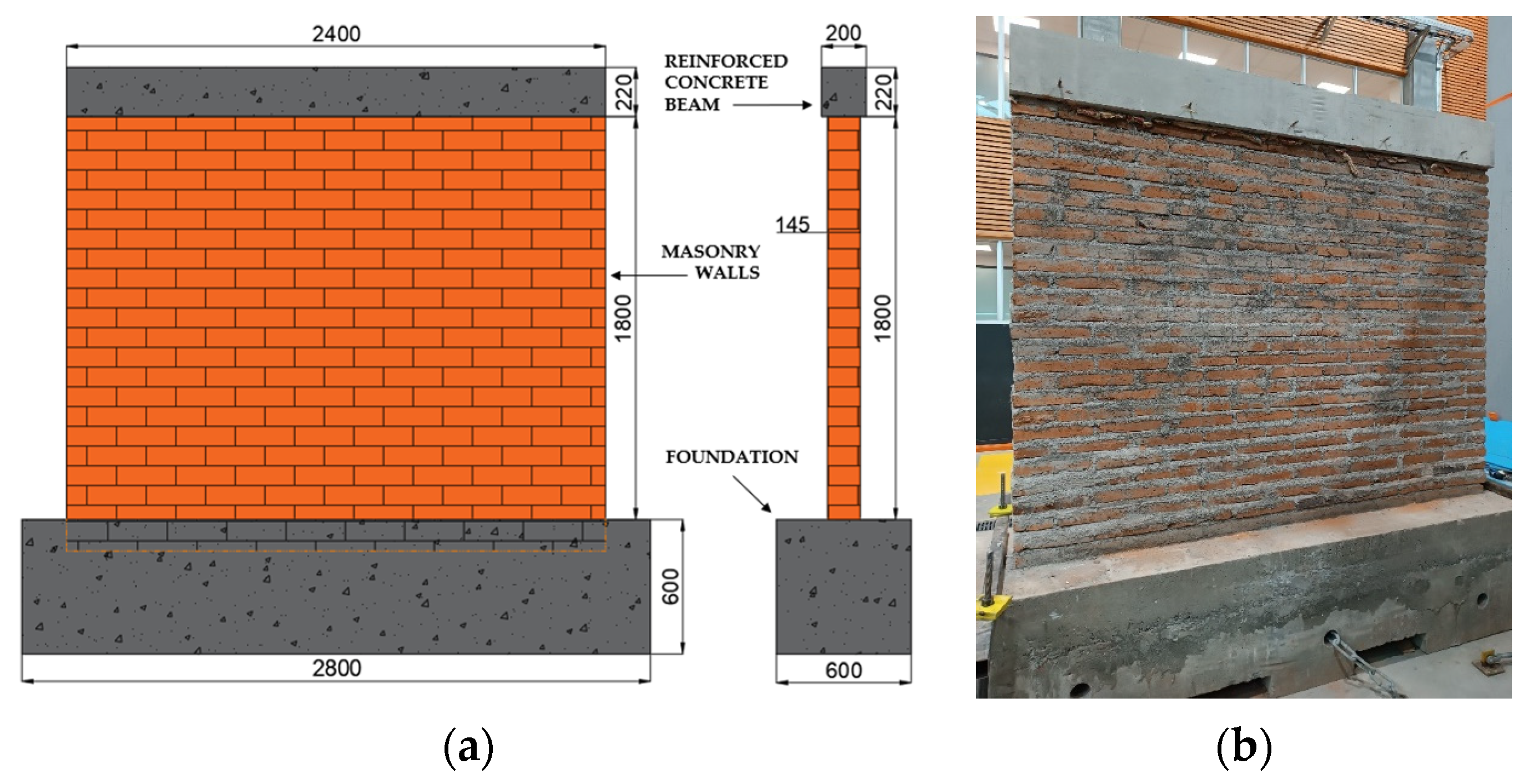
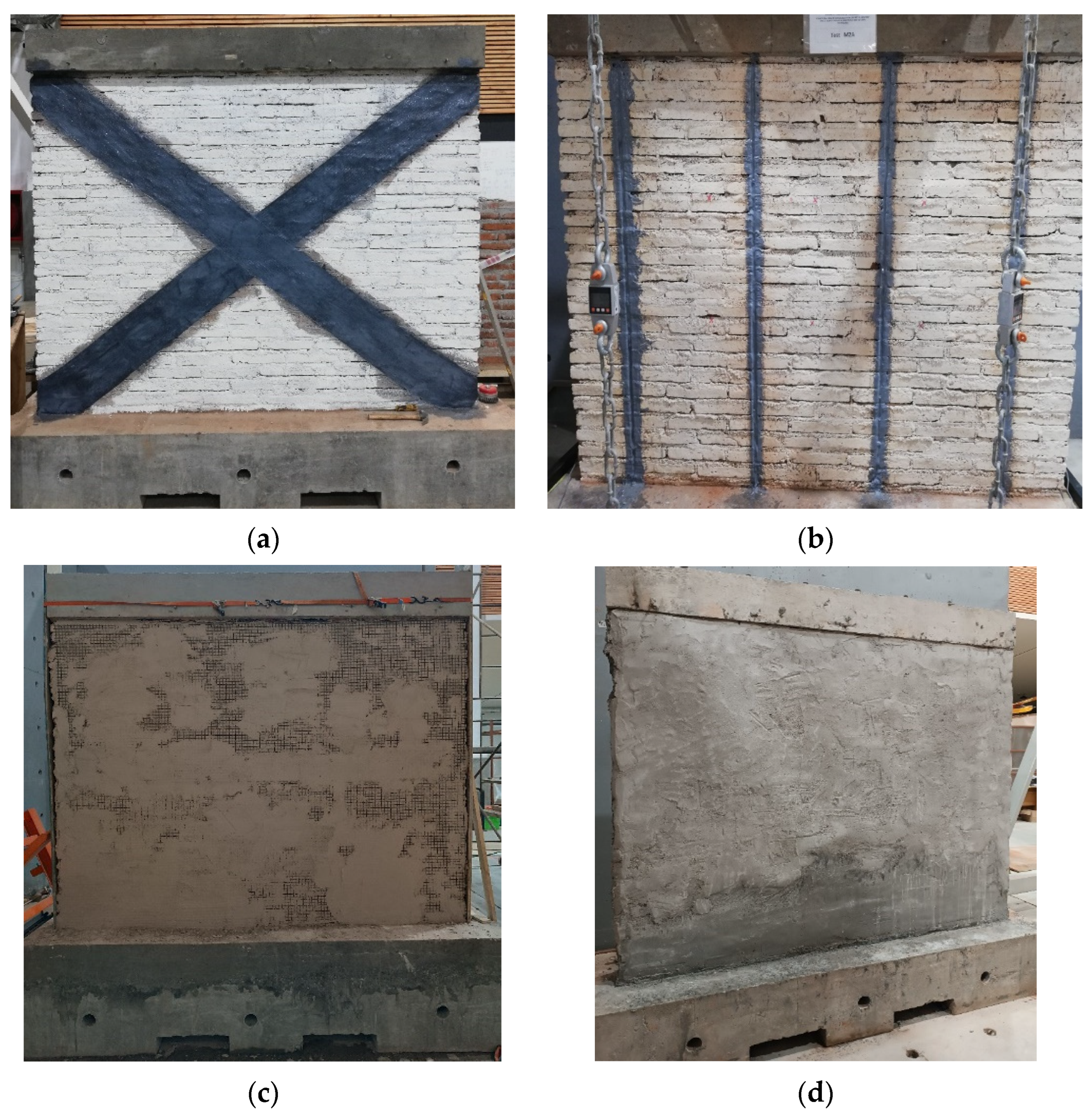
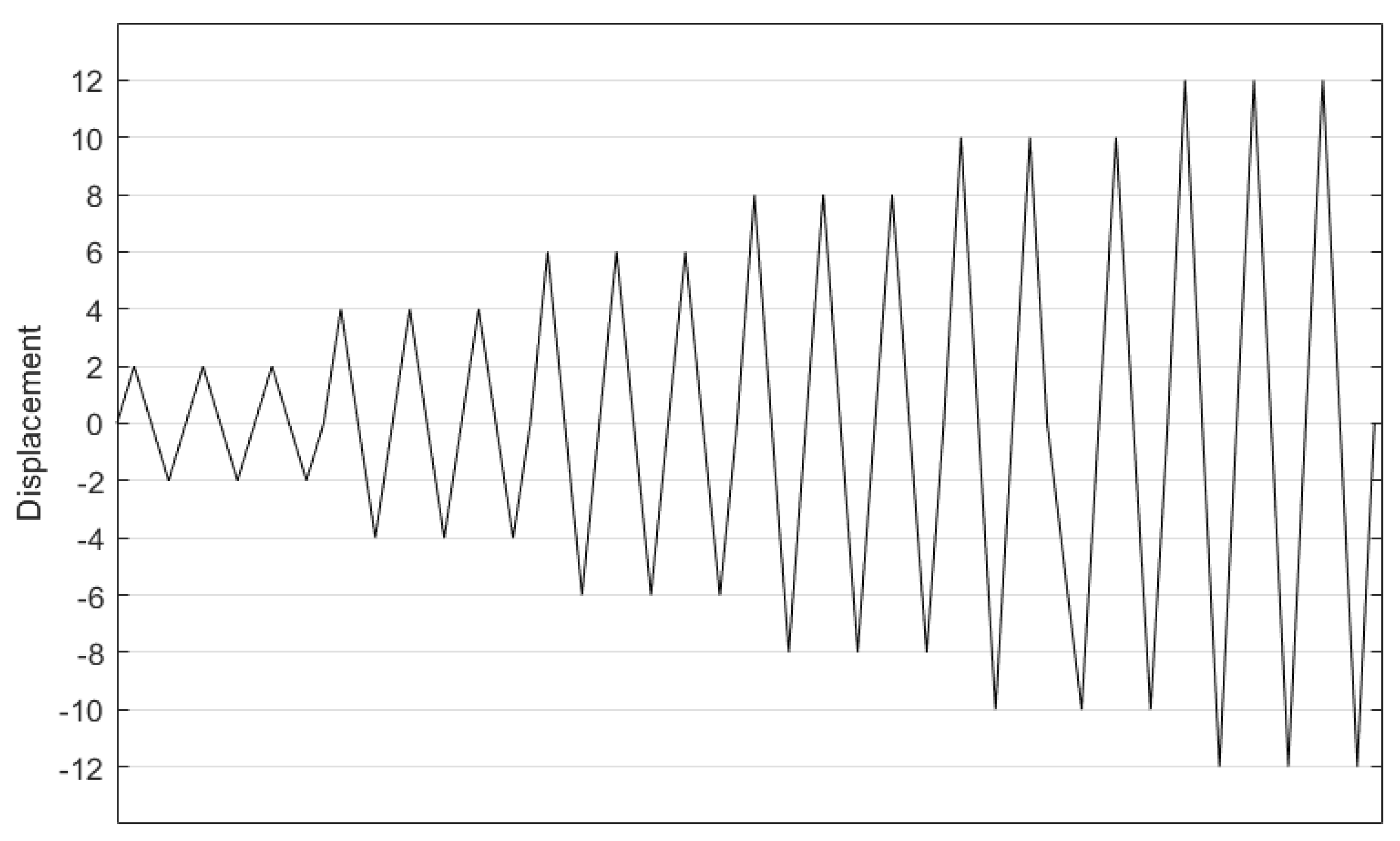

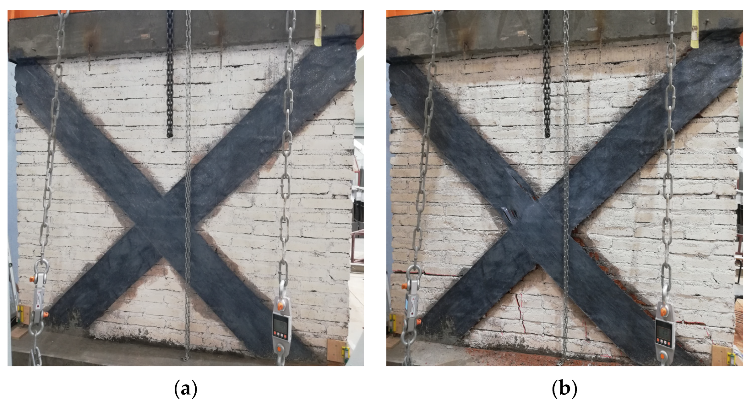
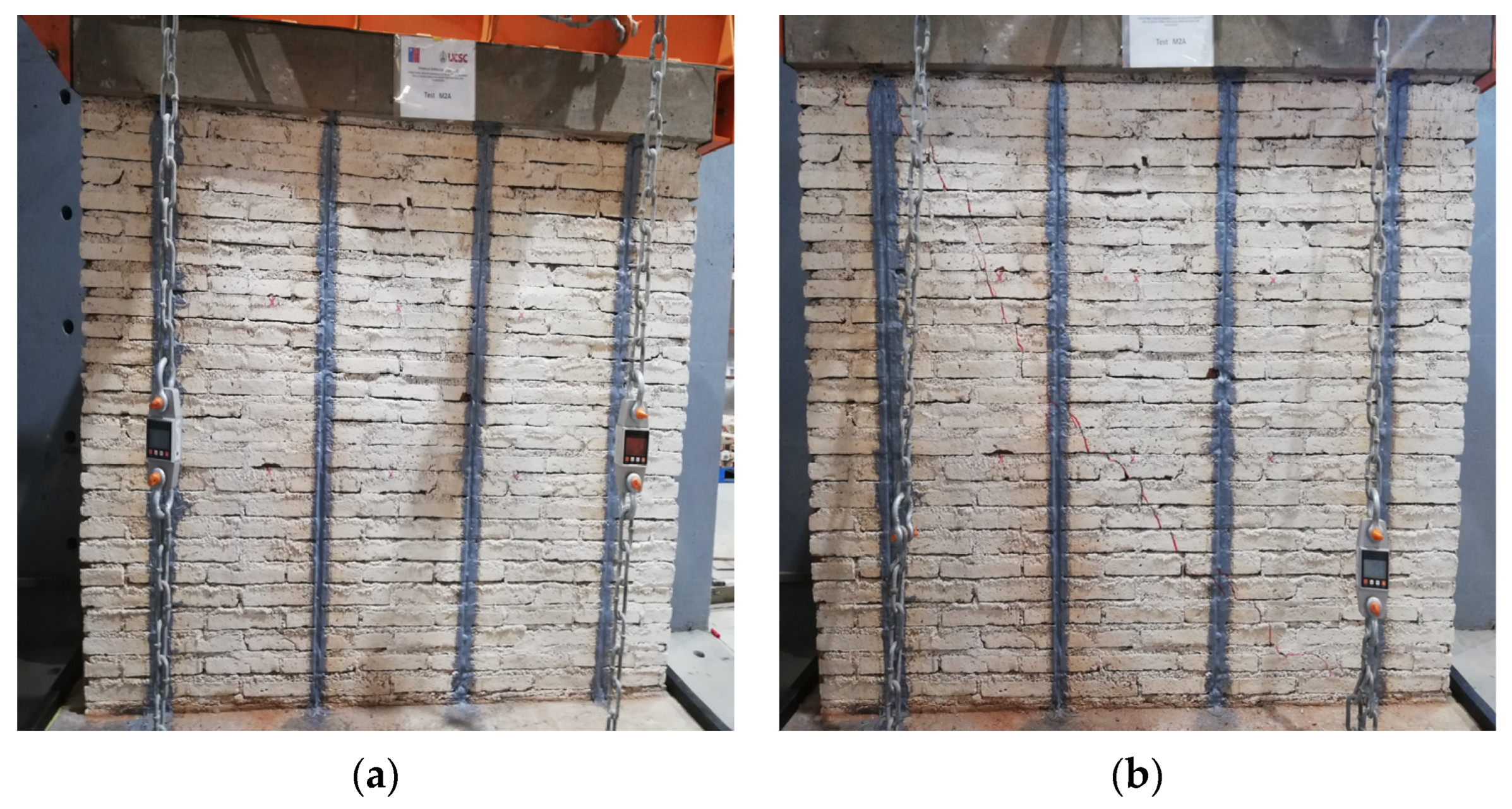

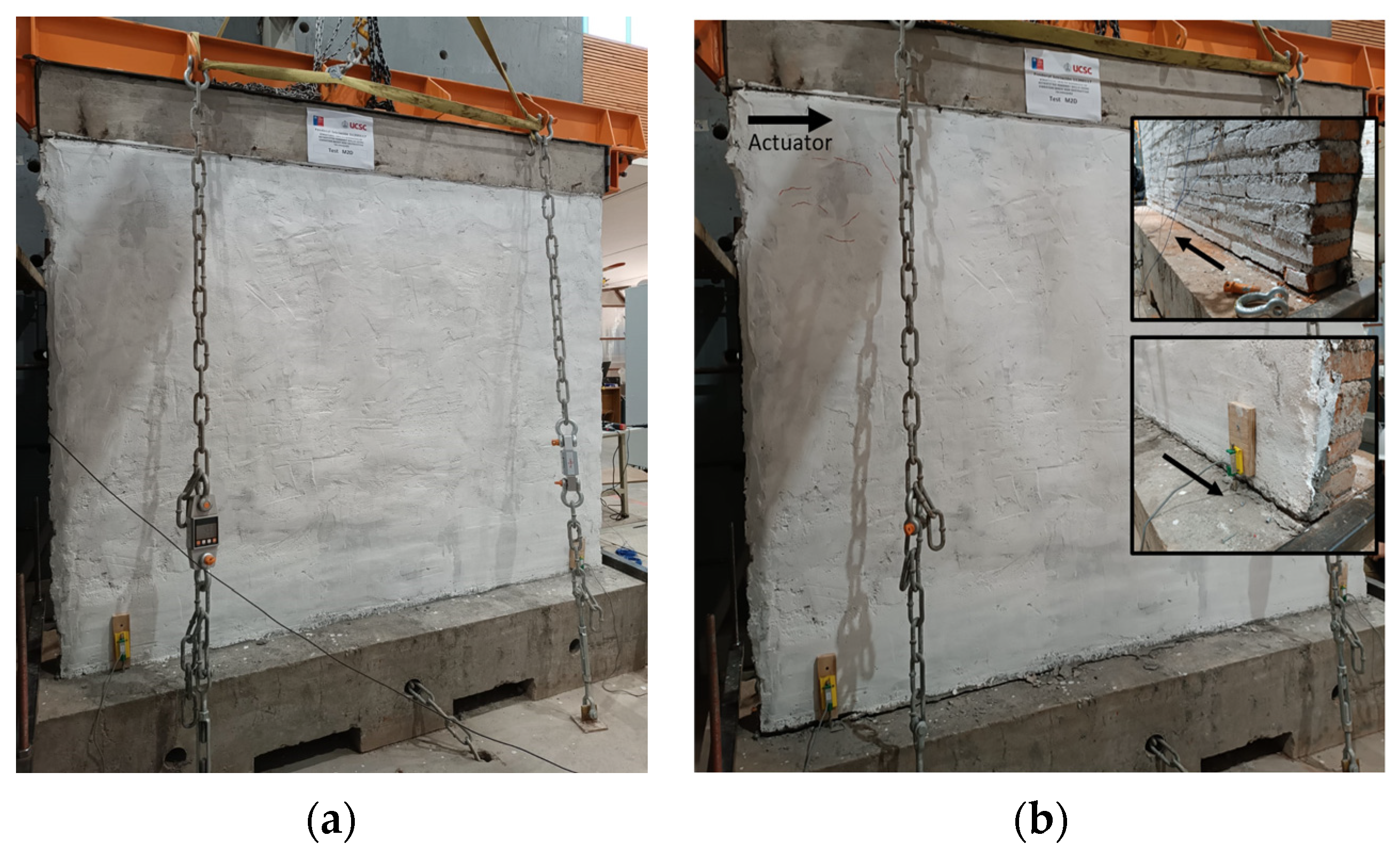
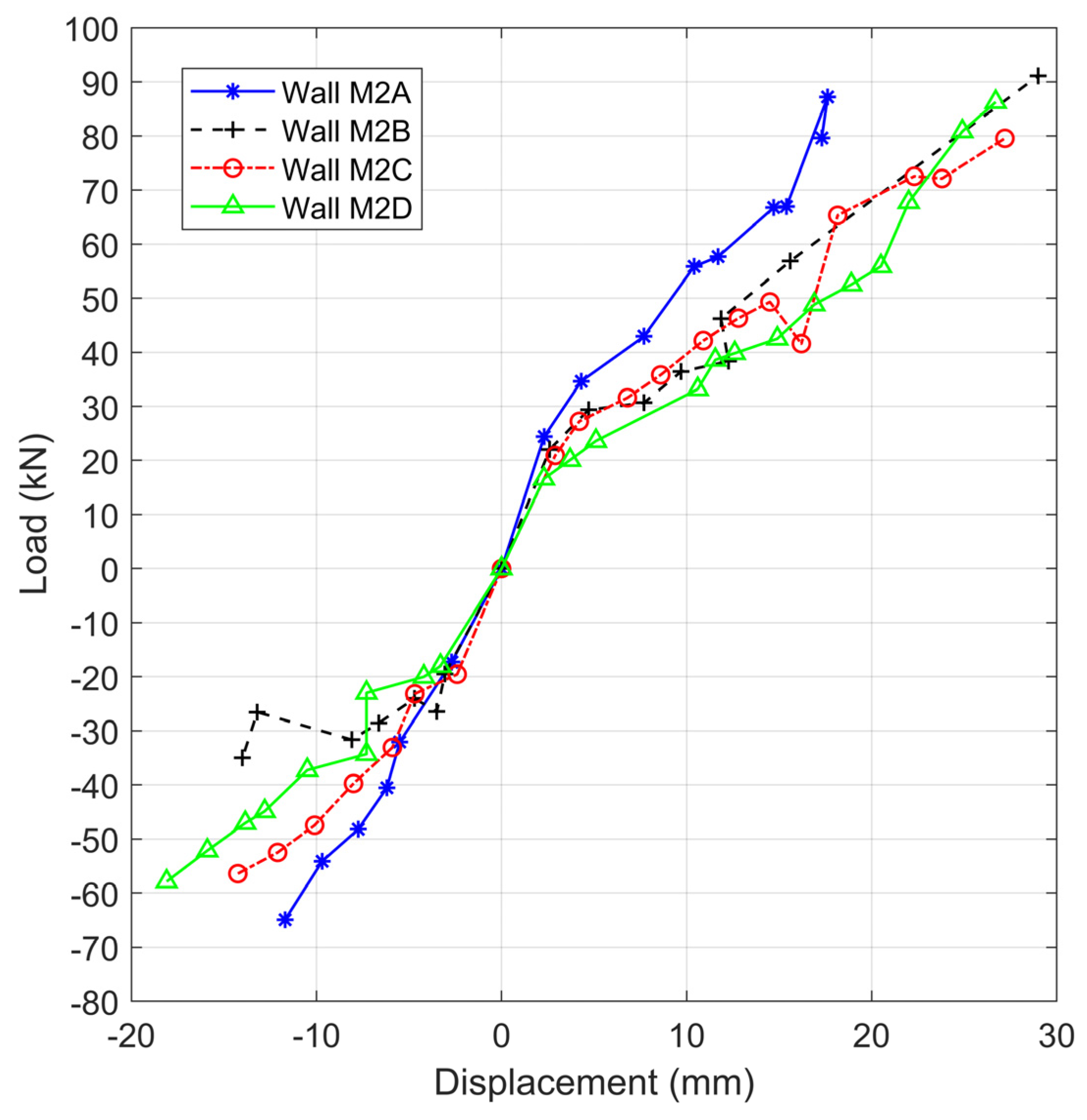

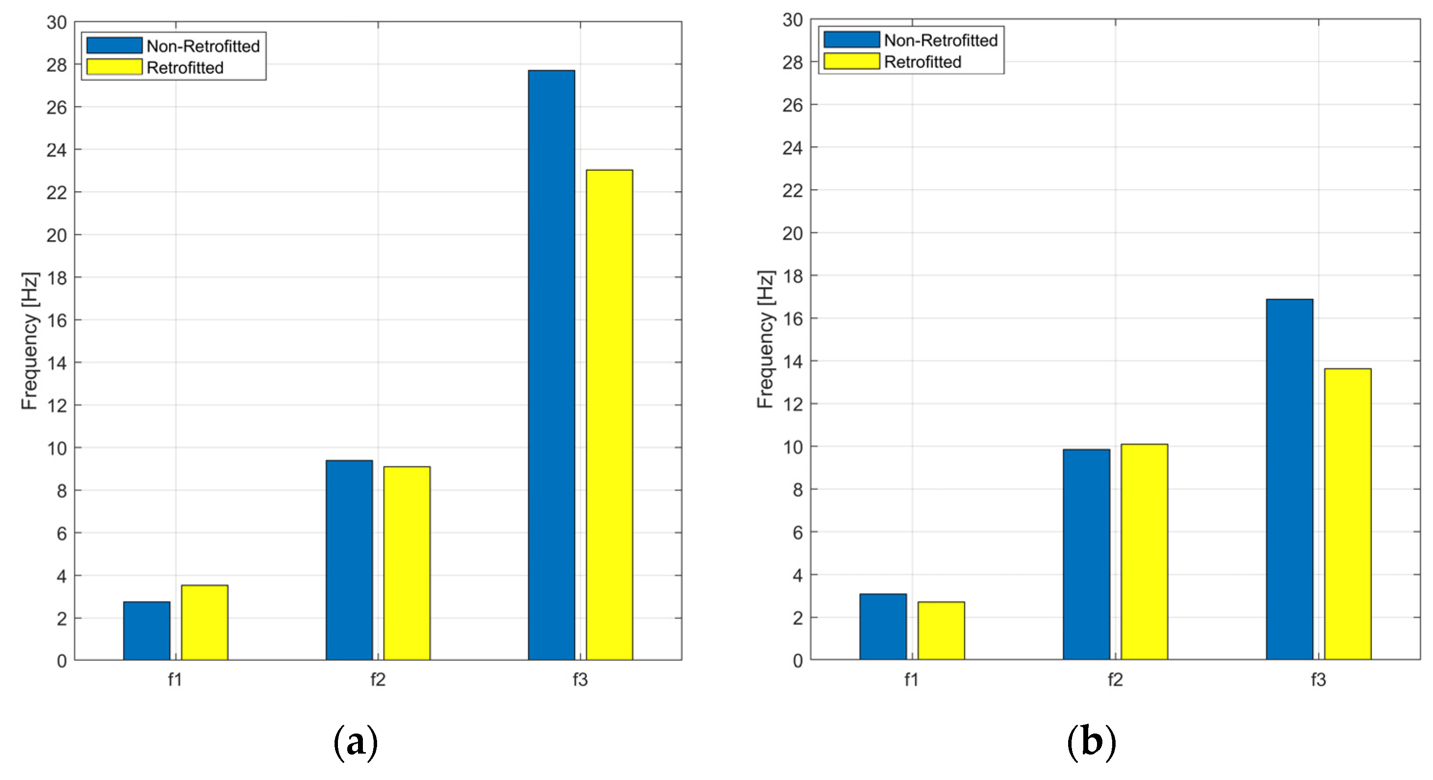

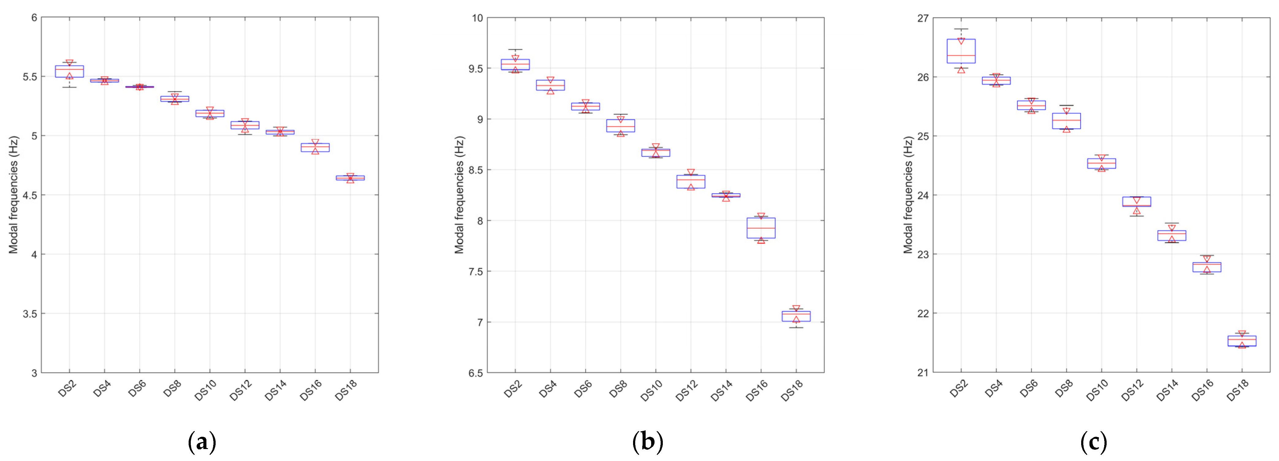
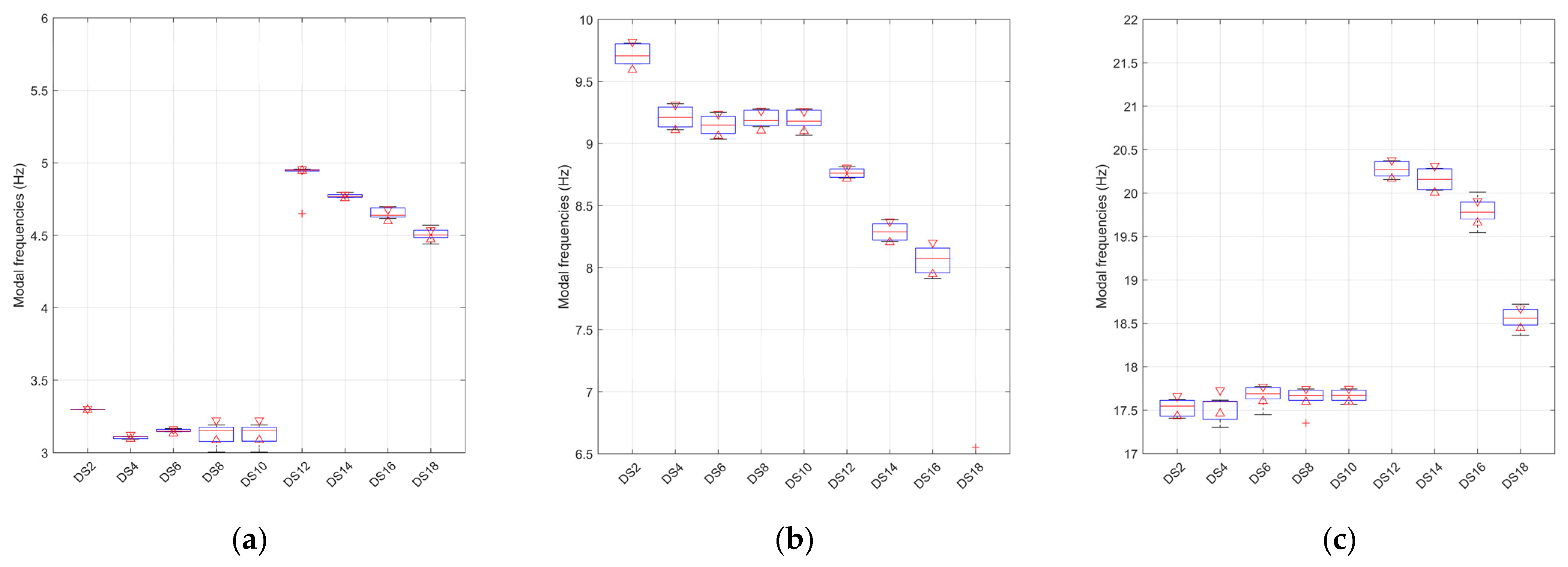
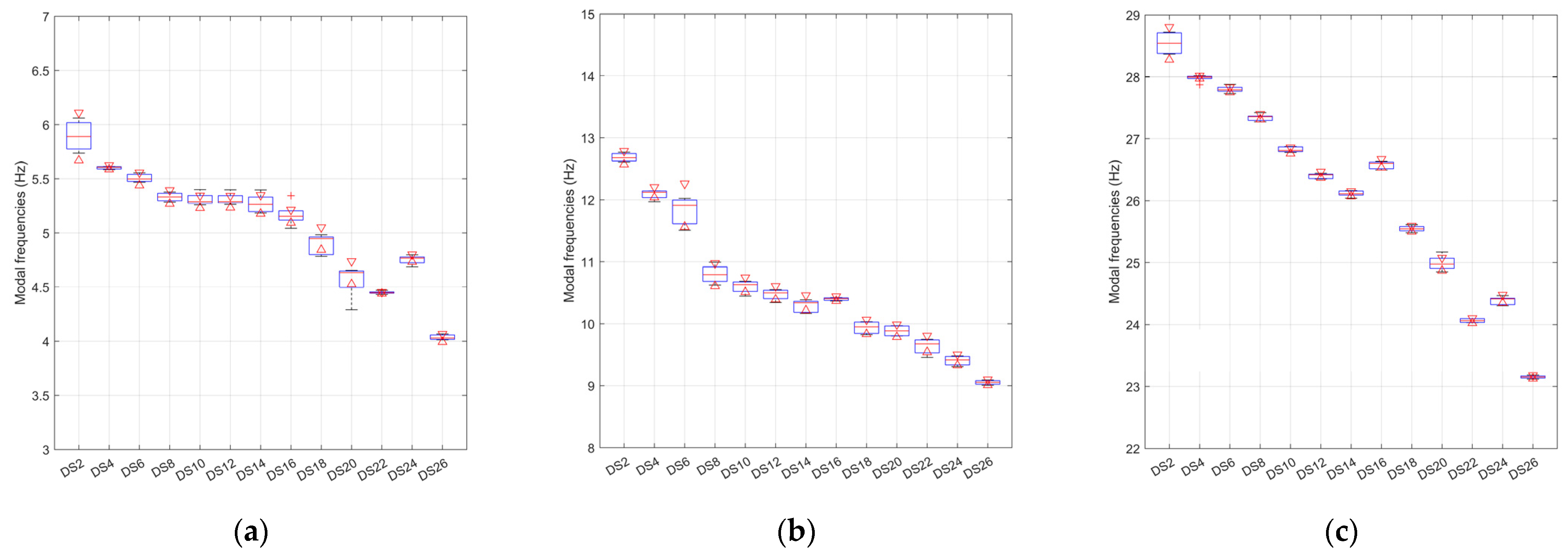
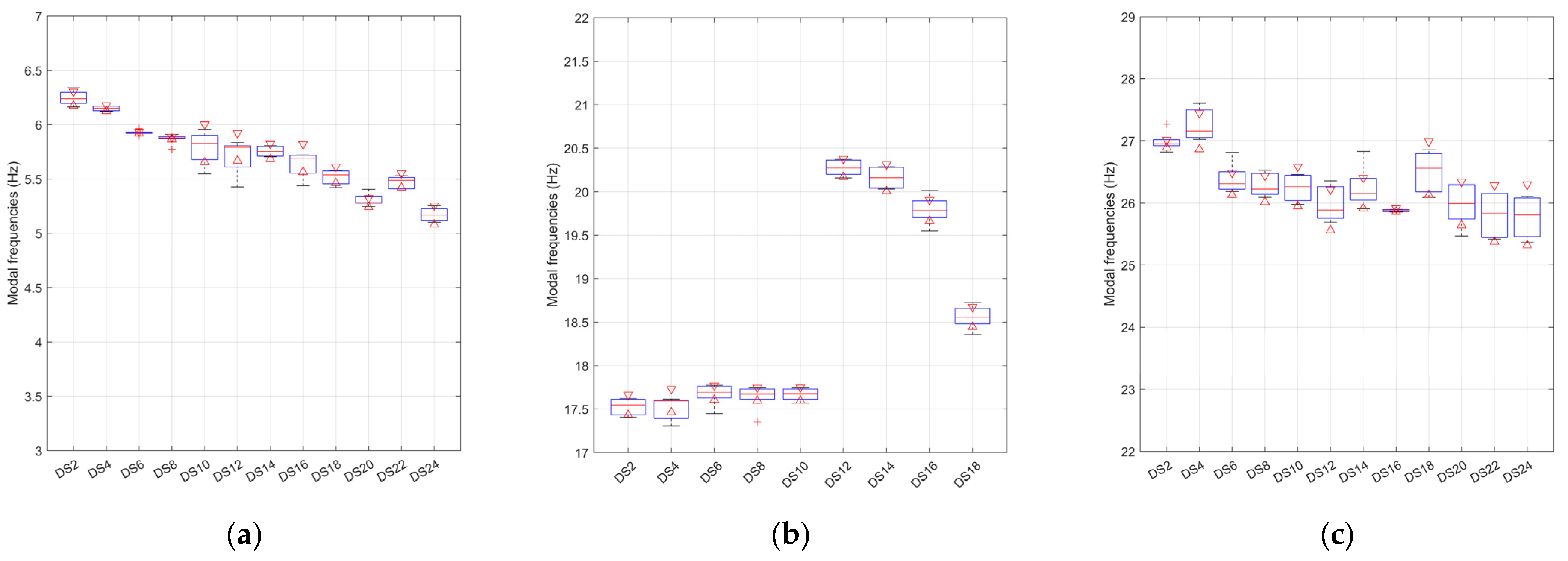
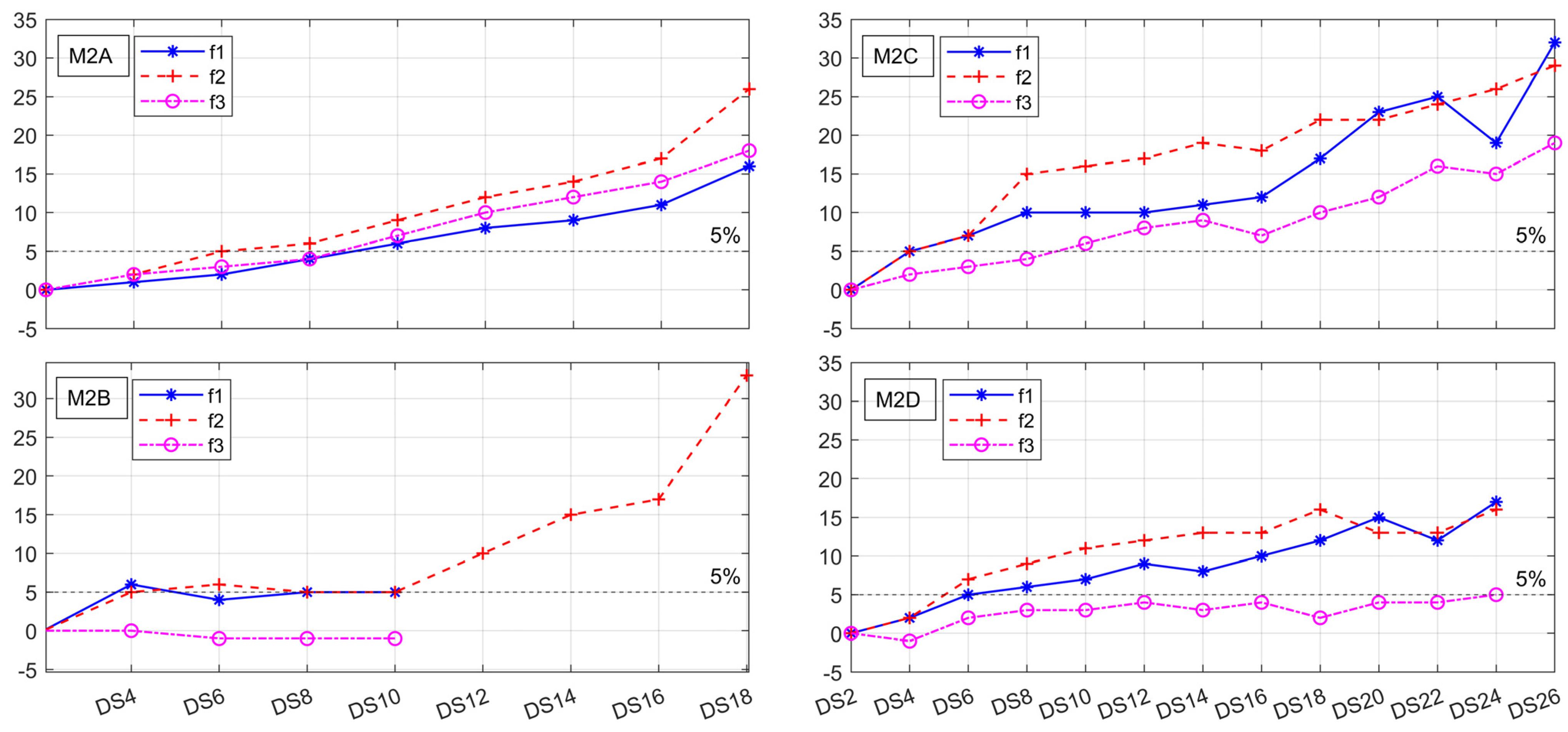
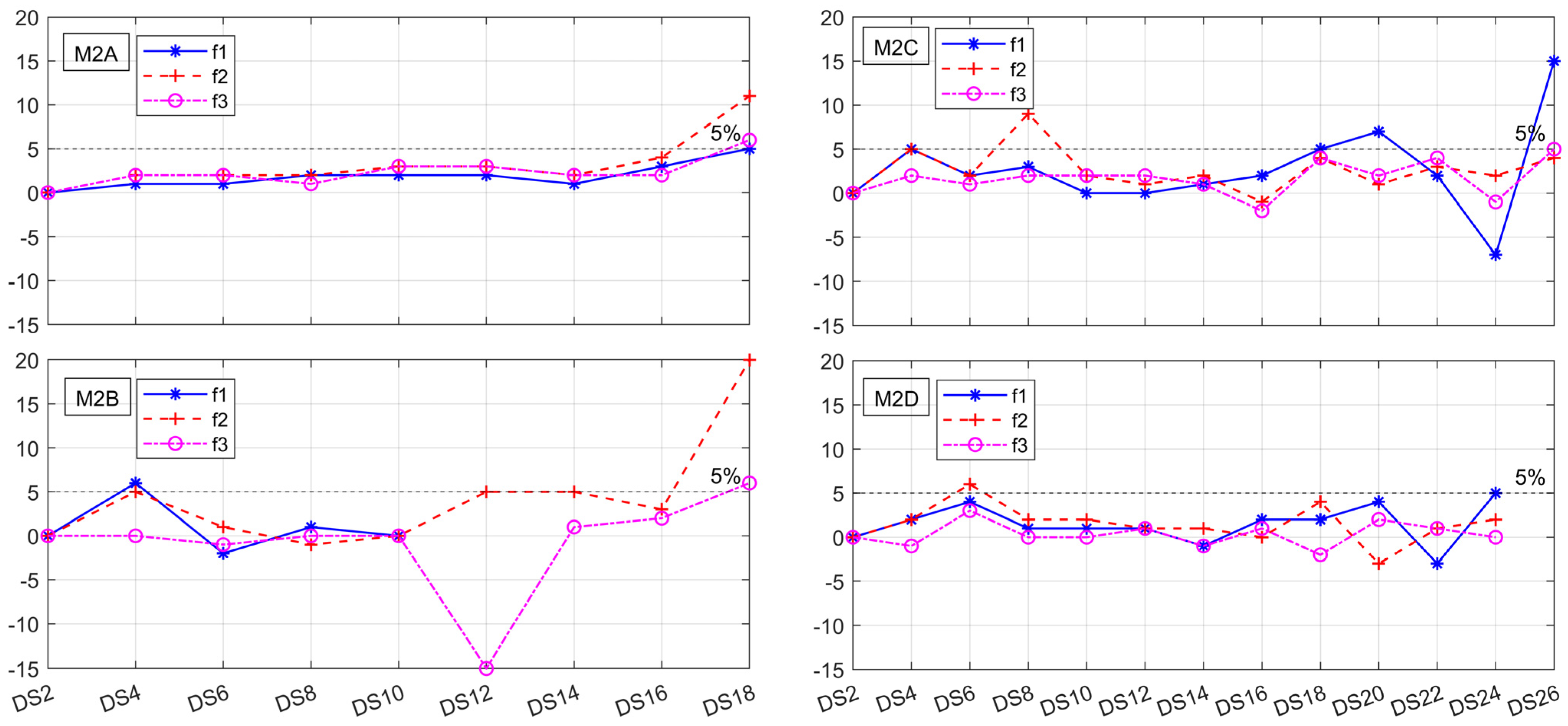
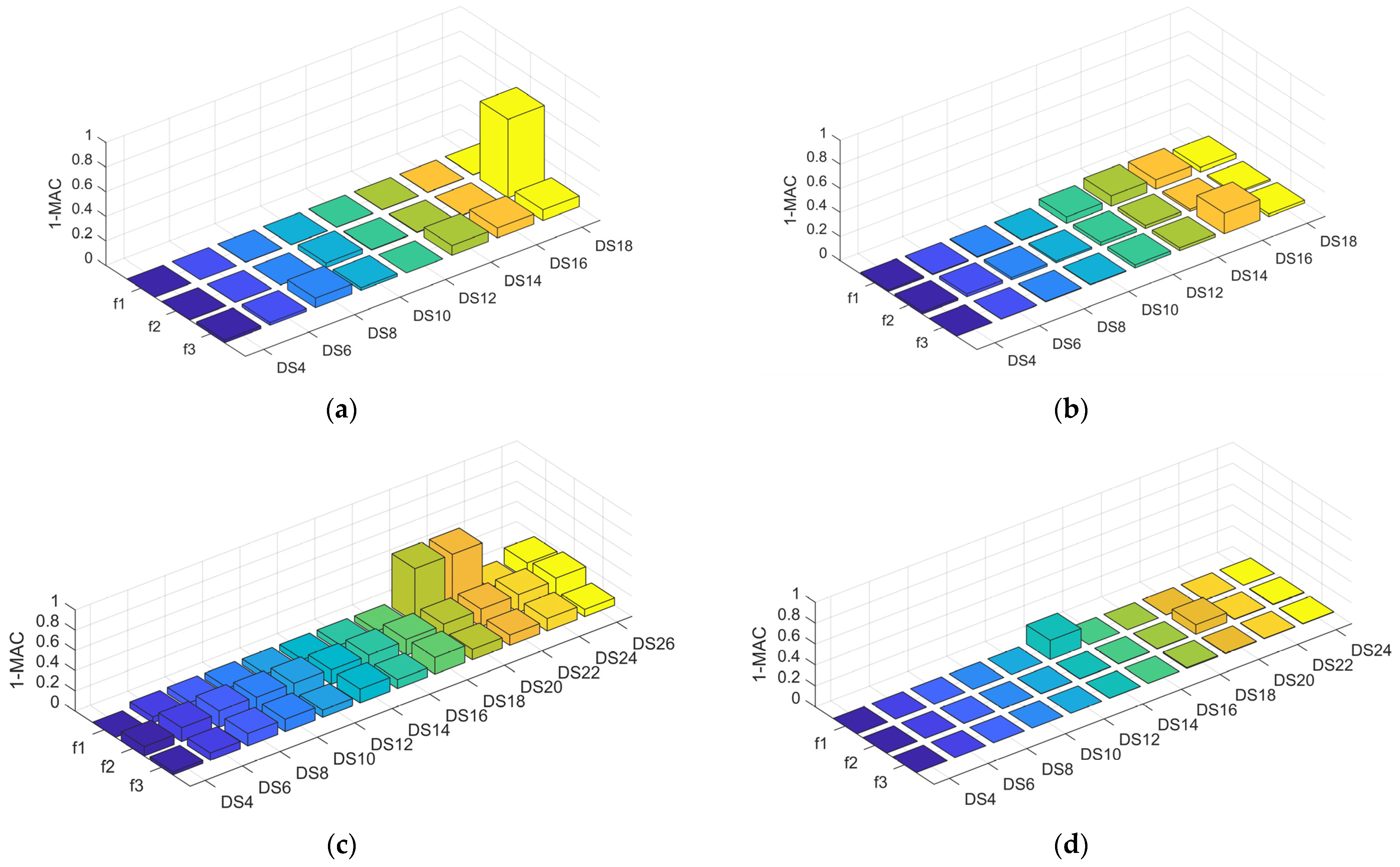
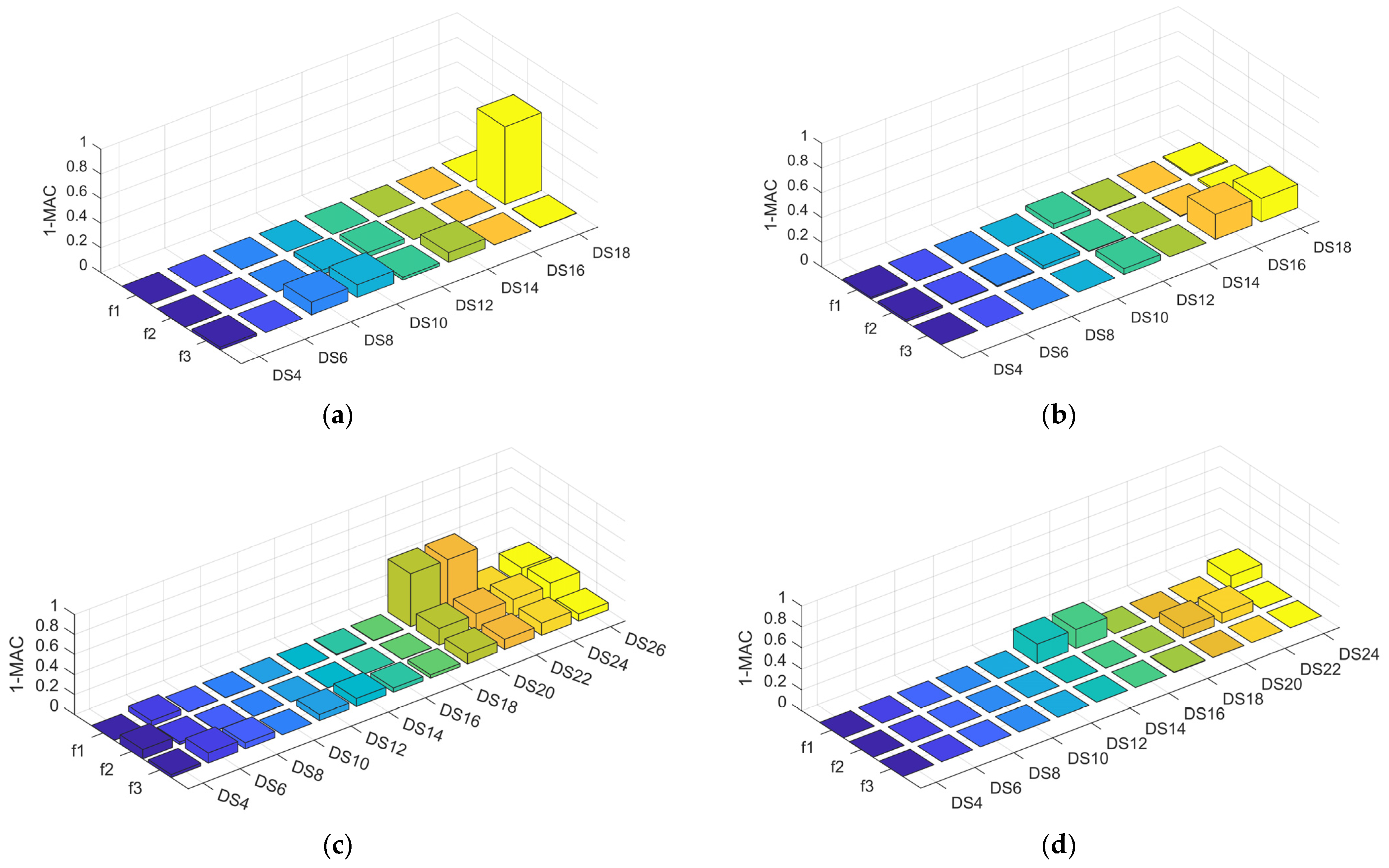
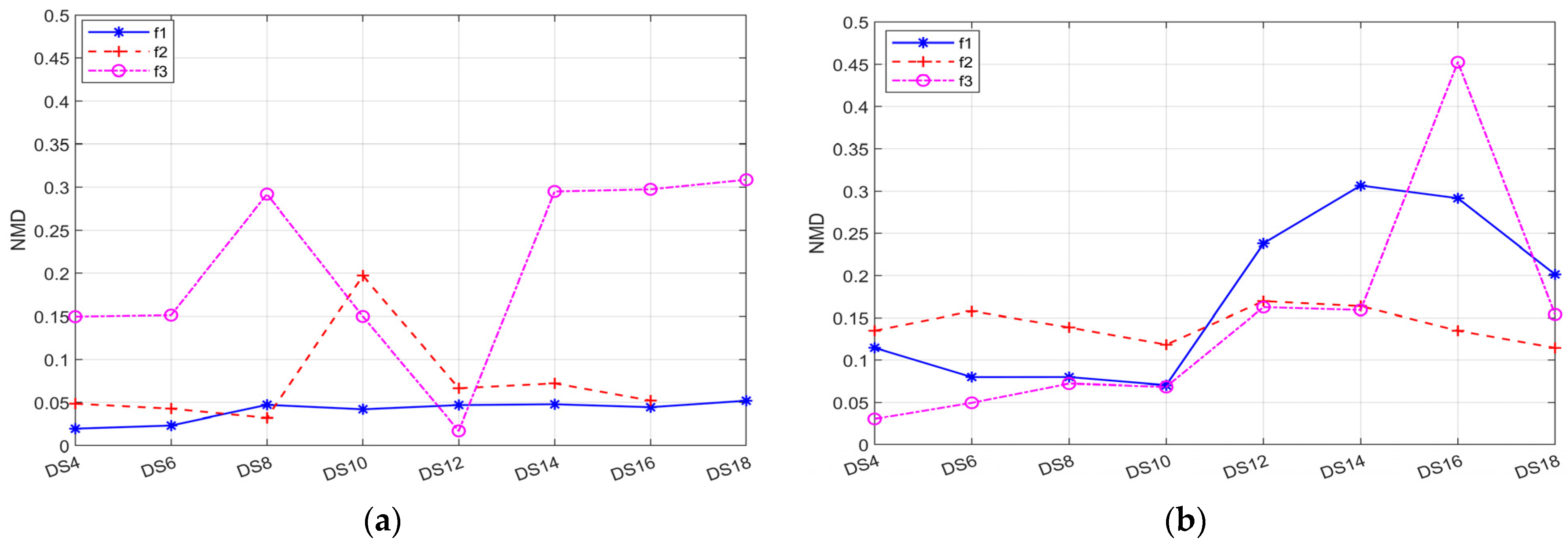
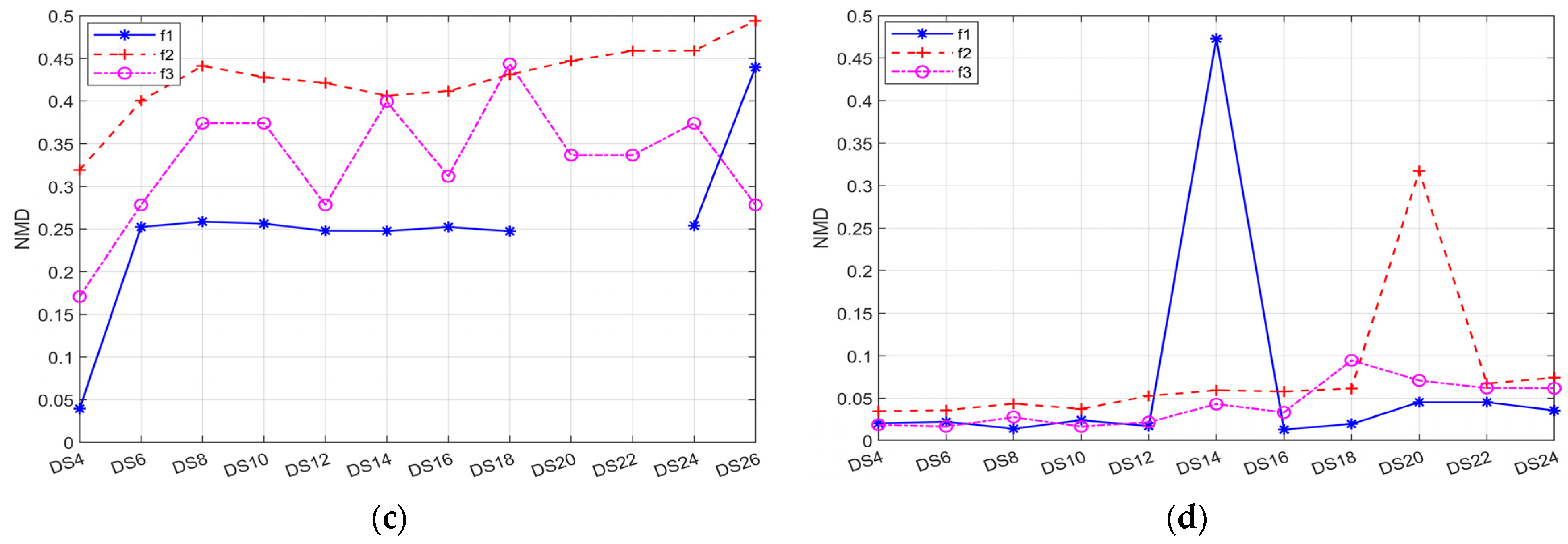
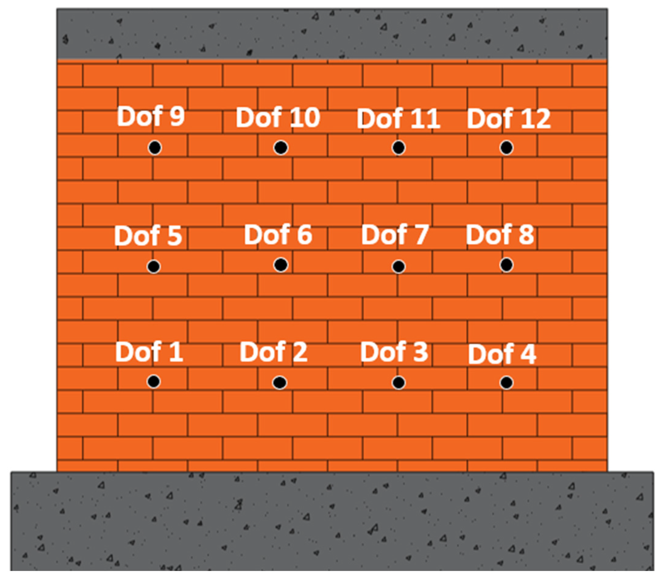

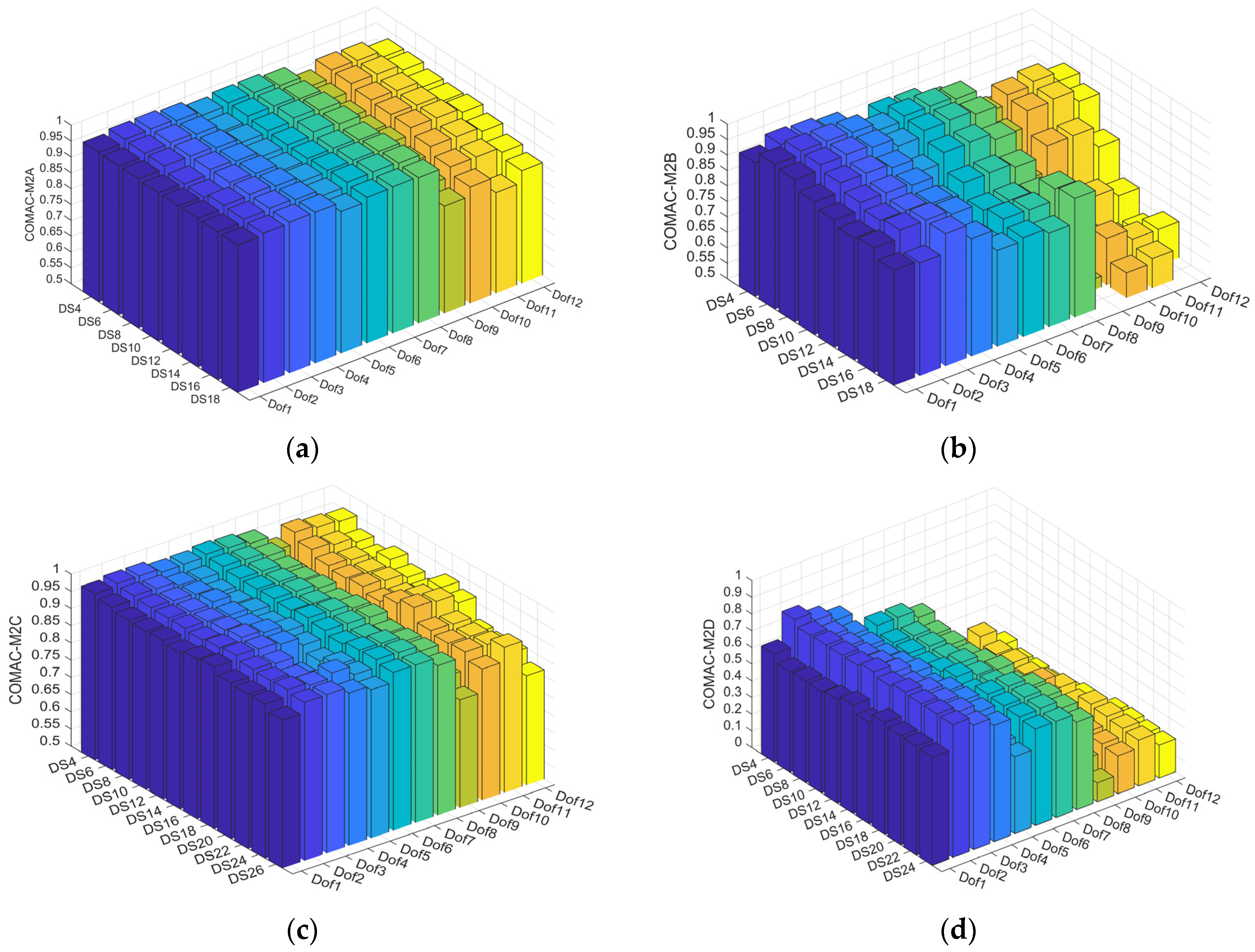
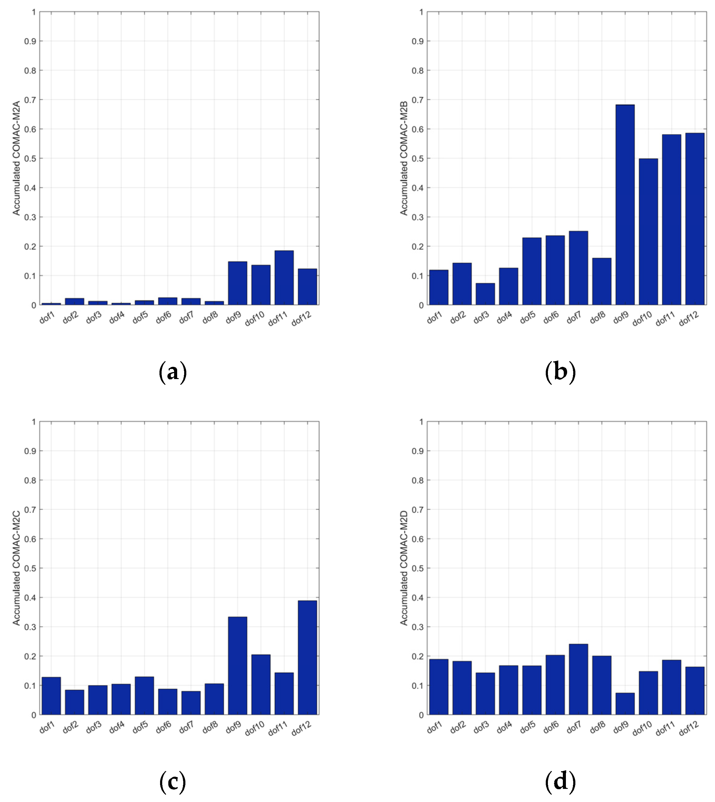

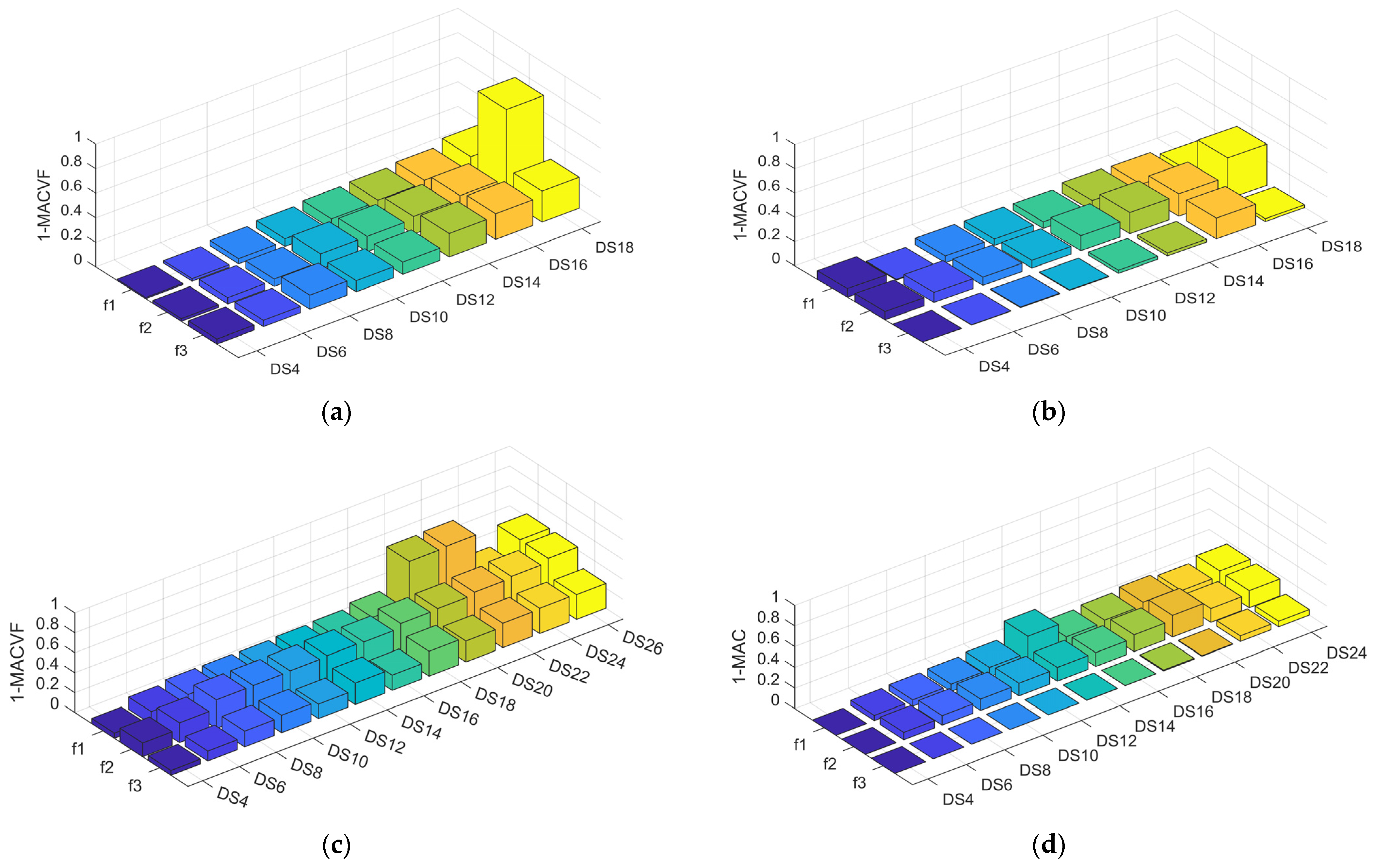

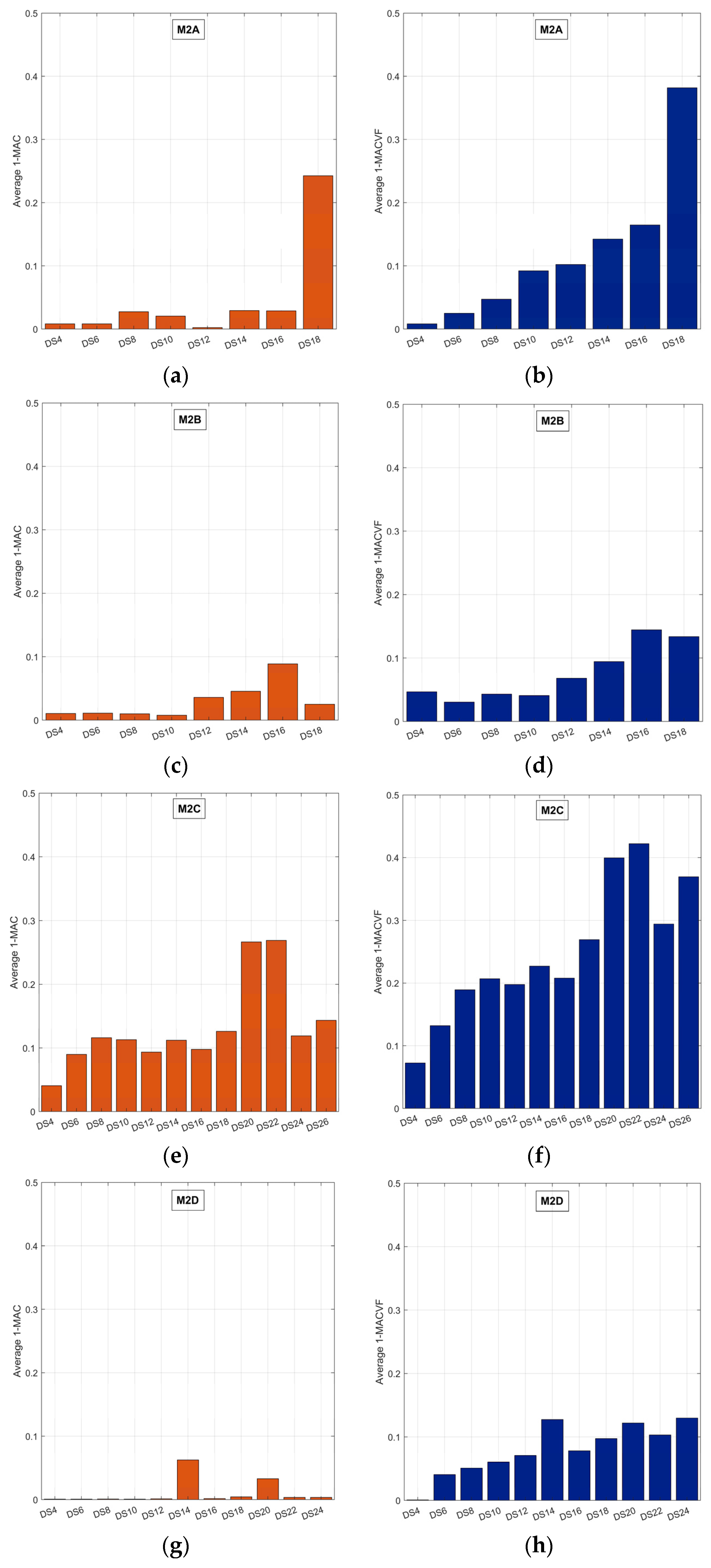


Disclaimer/Publisher’s Note: The statements, opinions and data contained in all publications are solely those of the individual author(s) and contributor(s) and not of MDPI and/or the editor(s). MDPI and/or the editor(s) disclaim responsibility for any injury to people or property resulting from any ideas, methods, instructions or products referred to in the content. |
© 2024 by the authors. Licensee MDPI, Basel, Switzerland. This article is an open access article distributed under the terms and conditions of the Creative Commons Attribution (CC BY) license (https://creativecommons.org/licenses/by/4.0/).