A Three-Step Computer Vision-Based Framework for Concrete Crack Detection and Dimensions Identification

Abstract

Crack detection is significant to building repair and maintenance; however, conventional inspection is a labor-intensive and time-consuming process for field engineers. This paper proposes a three-step computer vision-based framework to quickly recognize concrete cracks and automatically identify their length, maximum width, and area in damage images. In step one, a region-based convolutional neural network (YOLOv8) is applied to train the crack localizing model. In step two, Gaussian filtering, Canny, and FindContours are integrated to extract the reference contour (a pre-designed seal) to obtain the conversion scale between pixels and millimeter-wise sizes. In step three, the recognized crack bounding box is cropped, and the ApproxPolyDP function and Hough transform are performed to quantify crack dimensions based on the conversion ratio. The developed framework was validated on a dataset of 4630 crack images, and the model training took 150 epochs. Results show that the average crack detection accuracy reaches 95.7%, and the precision of quantified dimensions is over 90%, while the error increases as the crack size grows smaller (increasing to 8% when the crack width is within 1 mm). The proposed method can help engineers to efficiently achieve crack information at building inspection sites, while the reference frame must be pre-marked near the crack, which may limit the scope of application scenarios. In addition, the robustness and accuracy of the developed image processing techniques-based crack quantification algorithm need to be further improved to meet the requirements in real cases when the crack is located within a complex background.

1. Introduction

Concrete has been widely used in civil infrastructures such as buildings, bridges, and pavements due to its wide range of sources, simplicity of workmanship, and durability. Under prolonged exposure to loads and natural degradation, cracks may occur on the surface of the concrete structure, which in turn affects its reliability and safety [1]. Detecting and monitoring concrete cracks can provide effective information for structural repair and maintenance since cracks are one of the important indicators that characterize the load-bearing capacity. In most cases, crack detection still requires lots of manual involvement. However, these conventional inspection methods are time-consuming, inefficient, and costly, and they are also affected by the specialization and engineering experience of the inspectors [2].

Recently, computer vision and artificial intelligence have been recognized as key components in improving inspection methods in the field of structural health monitoring [3,4,5]. Vision-based algorithms combined with image or video capture devices offer new approaches for fast, accurate, and automatic detection of structural damages. Early image processing techniques used various statistical features, such as the original shape or edges of the damage image, to extract information for crack identification, classification, and regression. The techniques include edge detection [6], thresholding, filtering [7], etc.; however, they are sensitive to light variations and other noises in real environments. To enhance the detection robustness and optimize the performance, many studies have introduced machine learning methods, for example, support vector machines, directional gradient histograms, and local binary patterns [8,9], which still required tens of thousands of iterative steps and time-consuming pre- or post-processing operations [10].

Deep learning techniques have many advantages compared with traditional machine learning methods, especially in terms of accuracy and recognition speed, and are therefore increasingly being deployed in crack detection [11]. When training on damage images, an end-to-end convolutional neural network (CNN) is usually used to learn and generate crack recognition models [12]. The complex relationship between data can be fitted by parametric nonlinear functions, and the greater the number of nodes and hidden layers of a CNN, the easier it is to achieve parametric approximation [13]. Dang et al. [14] applied CNNs to image blocks to automatically detect bridge surface damage captured by a remotely operated unmanned aerial vehicle (UAV). Kim et al. [15] combined CNN and binarization operations to identify cracks in concrete components and locate the pixel regions of the cracks. In addition, researchers have proposed some crack detection approaches based on AlexNet [16], VGG [17], and ResNet [18]. In order to improve the recognition efficiency and accuracy further, the regional convolutional neural network (R-CNN) has been proposed, which divides the detection task into feature pre-training, classification prediction, and bounding box regression [19]. However, these methods are incapable of segmenting the specific shape of cracks since they can only identify the bounding box of the region of interest.

In building inspections, quantifying the damage degree is a critical step that can help engineers evaluate the remaining life of structures. To achieve more feature information, some studies have applied vision-assisted techniques to measure the damage dimensions [20,21,22], such as semantic segmentation of cracks at different scales using fully convolutional neural networks [23]. Attard et al. [24] proposed a method based on Mask R-CNN [25] to locate cracks on concrete surfaces and obtain corresponding masks to help segment shapes. Liu et al. [26] developed a model based on U-Net to depict the shape and direction of cracks automatically. YOLO (You Only Look Once) is a deep neural network-based target detection algorithm that has been widely used in computer vision due to its high speed and accuracy [27]. Therefore, several studies have developed algorithms to identify cracks based on YOLO, such as the improved YOLOv3 [28,29], YOLO-tiny [30], etc. Although the dimensions like the length and width of the cracks can be derived from these methods, the measuring results are pixel-wise rather than real millimeters. In order to capture the real dimensions of the damage, researchers have proposed reference-based image analysis methods, including transformation between pixel coordinates and real-world coordinates through chevron plane-plate calibration [31] or using a binocular camera to acquire the true depth of the damage through stereo vision approaches [32]. Nevertheless, the above methods are relatively complex to operate reliably on additional equipment and are also susceptible to surrounding environments that may result in compromised detection accuracy.

With the aim of improving the robustness of crack recognition and realizing fast, accurate, and convenient quantification of real-world millimeter-wise dimensions in housing quality inspections, this paper proposes a three-step computer vision-based framework based on deep learning and fused image processing algorithms. The proposed framework first identifies the bounding box of each crack from images using the YOLOv8 target detection network. Secondly, the FindContours algorithm is applied for contour extraction of the reference frame, and scale conversion is performed to achieve the ratio between pixels and millimeter-wise sizes. Then, the target box is cropped, and the pixel-wise contour of the crack is extracted. Finally, its length and area are calculated based on the conversion ratio, as well as the maximum width obtained by the maximum internal tangent circle (CircleFit) algorithm. The general flowchart of the proposed framework is demonstrated in Figure 1.

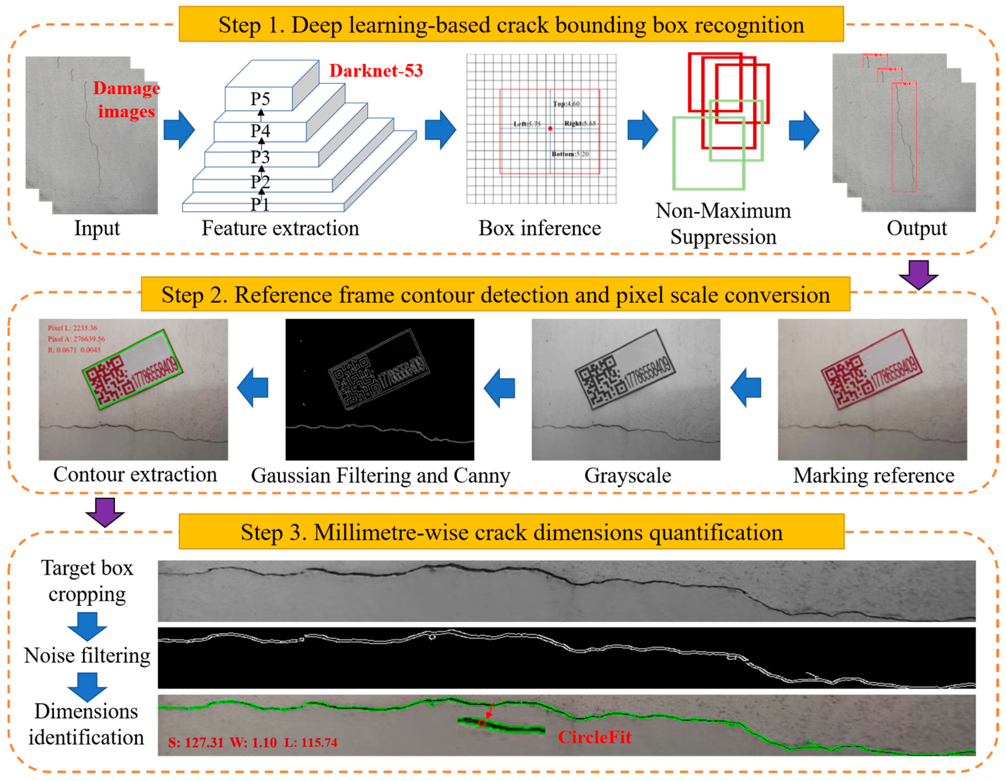
2. Methodologies

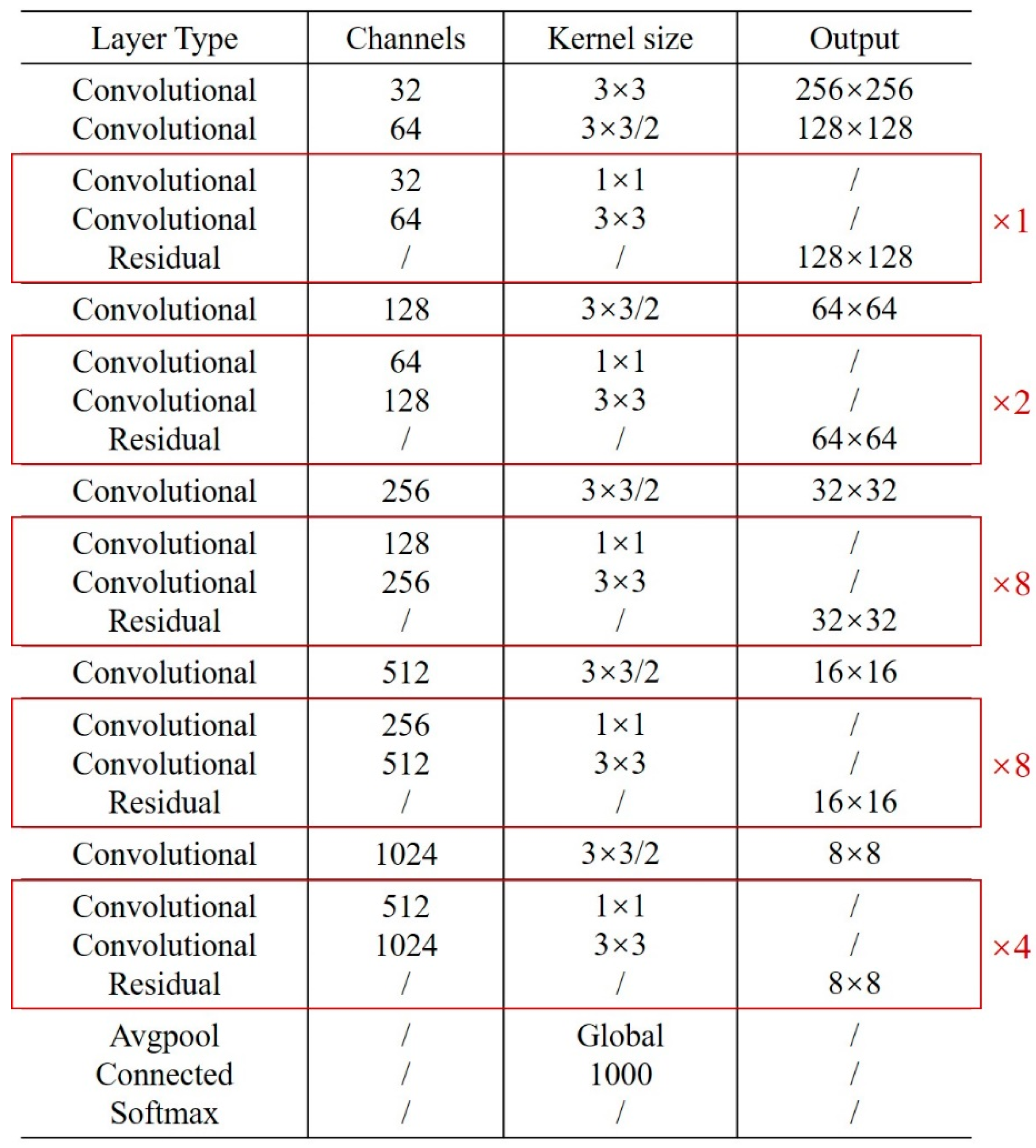
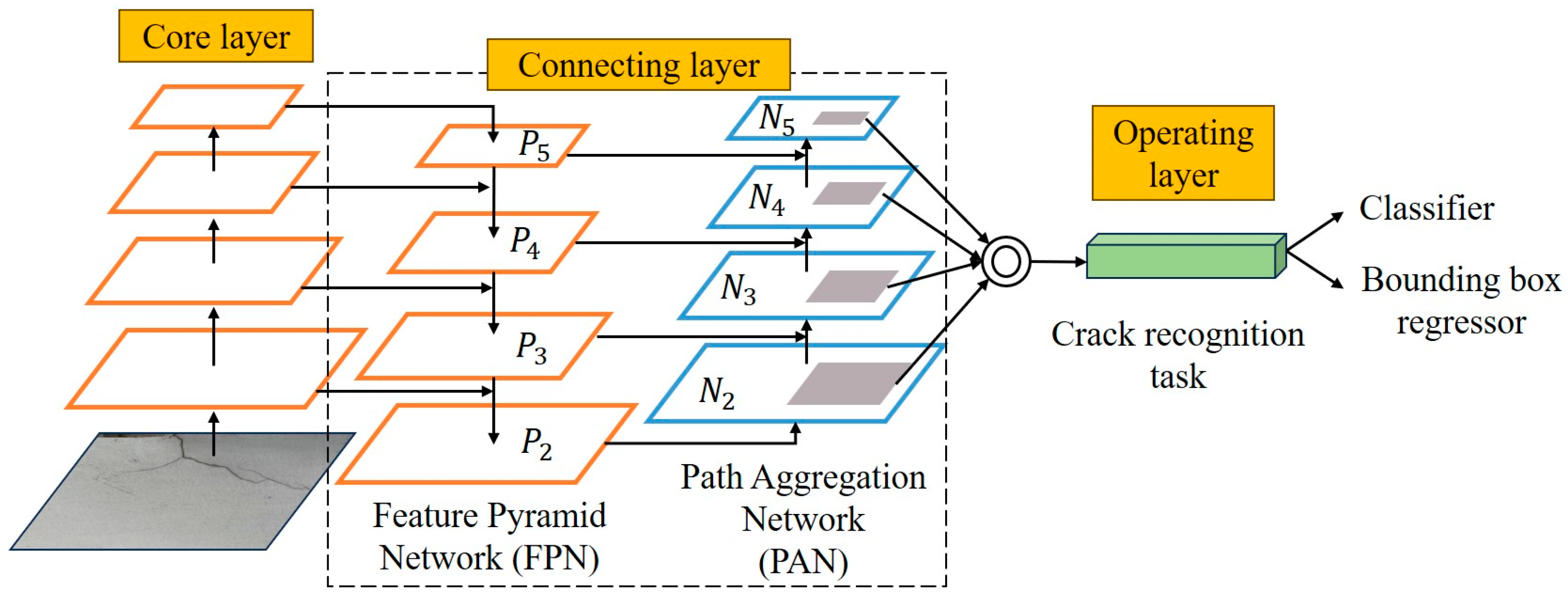
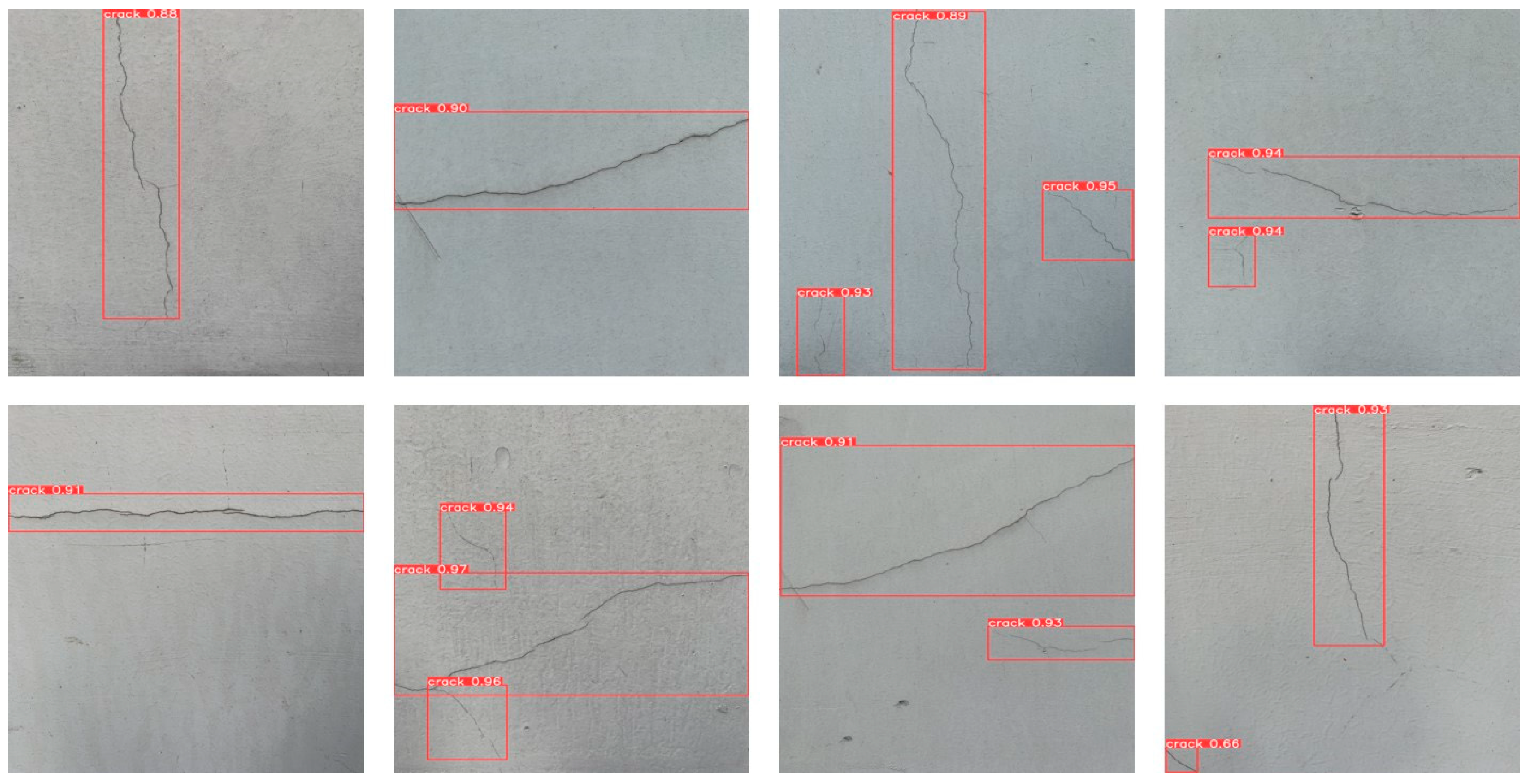
2.1. Deep Learning-Based Crack Recognition (Step One)

The series of YOLO target detection algorithms have received widespread attention for their efficient and accurate performance. Currently, the most advanced version is YOLOv8, which has been optimized and improved from its predecessor to make the model more flexible in predicting target locations [33]. In this research, the bounding box of each concrete crack in damage images is identified through the YOLOv8 deep learning algorithm. The core layer applies Darknet-53 [34] to extract feature maps, including five stages (convolution and residual block) and doubled channels after each pooling operation. The number of convolutional and residual layers, channels, kernel size, and output size of Darknet-53 are listed in Figure 2. The global average pooling is used to perform predictions, and a batch normalization layer acts as a regularizer to stabilize the model training as well as accelerate convergence.

Residual connections are extensively employed in the core layer so that the architecture can be designed deeply to alleviate the problem of vanishing gradients during the training process. In addition, downsampling is implemented by using a convolutional layer with a stride of two instead of a pooling layer. The convolutional module consists of convolution, batchnorm, and the SiLU activation function [35]. As shown in Figure 3, the input damage image undergoes a Feature Pyramid Network (FPN) that conveys the semantic features of the higher layers from up to down and then passes P3, P4, and P5 to the next operating and connecting layers to perform the crack recognition task. Since the process only enhances the semantic information without conveying the localization information, a bottom–top Path Aggregation Network (PAN) pyramid is added after the FPN as a complement to aggregate the shallow and deep feature maps, which delivers the localization feature information upwards along specific paths to further enhance the representation of multi-scale features.

The operating layer is the final layer of the algorithm, and the decoupled structure is used to separate classification and bounding box regression. The classifier is measured by the cross-entropy Varifocal Loss (VFL), which is formulated as follows:

$$L_{cls}=VFL(p,q)=\left\{\begin{array}{c}-q(q(\log (p)+(1-q)\log (1-p)),\hspace{1em}q>0\\ -\alpha p^{\gamma }\log (1-p),\hspace{1em}q=0\end{array}\right.$$

(1)

where q denotes the Intersection over Union (IoU) of the bounding (predicted) box and ground truth box; IoU is the intersection of the predicted and ground truth box divided by the concatenation of the two boxes; p refers to the score, i.e., probability.

The bounding box loss is divided into two loss functions: the Distribution Focal Loss (DFL) [36] and the CIoU Loss. DFL models the position of the box as a general distribution and optimizes the probability distribution of the left and right positions of the label y using a cross-entropy function, allowing the output distribution of the network to be more centrally focused around the label values:

$$DFL(S_i,S_{i+1})=-((y_{i+1}-y)\log (S_i)+(y-y_i)\log (S_{i+1}))$$

(2)

The CIoU Loss takes the aspect ratio of the bounding box into account, and its value is calculated as follows:

$$L_{CIoU}=1-IoU+{\displaystyle \frac{{\rho }^2(b,b^{gt})}{c^2}}+\alpha \upsilon$$

(3)

where b and b^gt denote the centroids of the bounding box and the ground truth box, respectively; ρ denotes the Euclidean distance between the two boxes; c refers to the diagonal distance between the closed regions of the two boxes; α means the weighting coefficients; v refers to the similarity of the aspect ratio (w/h) and is defined as:

$$v={\displaystyle \frac{4}{{\pi }^2}}{(\arctan {\displaystyle \frac{w^{gt}}{h^{gt}}}-\arctan {\displaystyle \frac{w}{h}})}^2$$

(4)

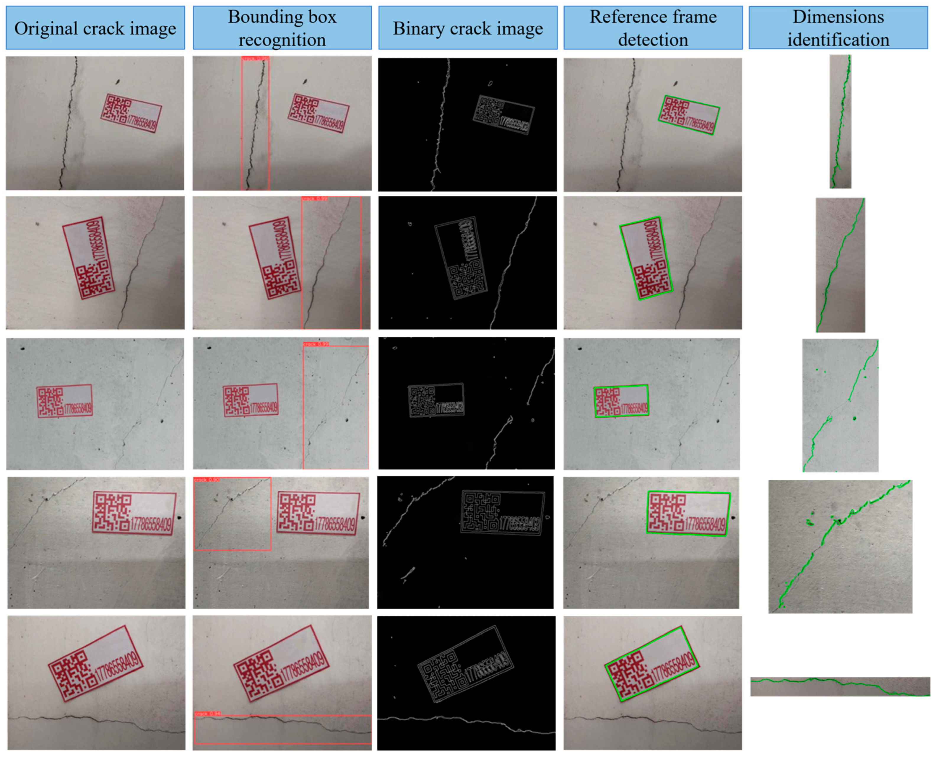
2.2. Fused IPTs-Based Reference Frame Contour Detection (Step Two)

In order to capture the millimeter-wise length, area, and maximum width of cracks a reference is required for scale conversion between image pixels and the millimeter-wise dimensions. The proposed method designs a seal as the reference frame, and its size is previously known to be 25 × 50 mm. In this research, the main application scenario considered is the housing quality inspection, and since most of the houses are buildings with flat facades, the seal was designed as a reference. The seal contains a QR code and the inspector’s contact information, with a blank section to add the inspector’s name. With the seal, crack dimensions can be detected directly by scanning the QR code during an on-site inspection, allowing even non-professional inspectors, such as ordinary residents, to access the information.

The reference contour detection is completed by following procedures: (i) Marking the seal adjacent to the crack to be detected; (ii) Greyscaling the input damage image that contains the complete reference frame to change it from RGB three-channel to single-channel; (iii) Using Gaussian filtering and Canny gradient algorithms to detect the strong and weak edges of the image; (iv) Applying FindContours to extract the reference frame contour, and using the ApproxPolyDP polygonal fitting function to approximate the contour by removing nearby redundant points; (v) Obtaining the pixel-level perimeter and area of the approximated contours, and computing the conversion ratio based on the millimeter-wise dimensions of the seal.

2.2.1. Image Greyscaling and Filtering

The input crack image is first resized to 600 × 600 pixels and then greyscaled to simplify the subsequent data processing and reduce the amount of calculation. There are four common methods for image greyscale processing: component method, maximum value method, average method, and weighted average method. In this study, the weighted average method is applied to convert the point pixels with coordinates (x, y) in the original damage image to grey pixels by averaging the weights of the R, G, B:

$$gray(x,y)=0.299\ast red(x,y)+0.587\ast green(x,y)+0.114\ast blue(x,y)$$

(5)

After converting the damage image to a greyscale image, Gaussian filtering [37] is conducted before crack dimensional quantification, as the background may lead to additional noise. The Gaussian filter is a linear filter that is widely used for image noise cancellation, and the larger the value of its standard deviation, the smoother the filtering performance. The developed method uses a (3, 3) Gaussian kernel as a template to scan each pixel in the damage image, and a weighted average is then applied to the whole image. Subsequently, the strong and weak edges of the image are detected by the Canny non-differential edge detection algorithm, and the damage image is scanned by non-maximal suppression to remove the points that do not belong to the edges. If the point belongs to the edge, it is labeled as white; if it does not belong to the edge, it is labeled as black. In the process of generating the binary image boundary, a fuzzy threshold [38] is used to determine whether the point is connected to the real boundary or not, and in this research, the minimum and maximum thresholds are set to 50 and 210, respectively. The peripheral contour of the seal (reference frame) is extracted after the above procedures.

2.2.2. Reference Frame Contour Extraction and Scale Conversion

The FindContours algorithm [39] adopted in this study only targets greyscale binary images. Row 0, row 599, column 0, and column 799 pixels form the borders of the damage image, where pixels with greyscale values of 0 and 1 are called 0 and 1 pixels, respectively. The four-connected domains of each pixel point are the top, bottom, left, and right adjacent positions of the corresponding pixel point (Figure 4a), and the eight-connected domains are the top, bottom, left, right, top-left, top-right, bottom-left, bottom-right adjacent positions and diagonal neighborhoods of the corresponding pixel point (Figure 4b). When there are all 0-pixel points in the connectivity domain, it is called a 0-connectivity domain; when there are all 1-pixel points in the connectivity domain, it is called a 1-connectivity domain. In a four-connected scene, if a 1-pixel eight-connected domain has 0 pixels, the point is judged to be a boundary point, and the boundary is composed of multiple boundary points. The interpretation of each boundary is shown in

Table 1. Interpretation of boundaries in the FindContours algorithm.

Boundaries	Interpretation
External boundary	Let S1 be a 1-connected domain and S2 be a 0-connected domain, the boundary between S2 and S1 is the external boundary when S2 directly surrounds S1.
Hole Boundary	Let S1 be a 1-connected domain and S2 be a 0-connected domain, the boundary between S1 and S2 is a hole boundary when S1 directly surrounds S2.
Parental Boundary	Let S1 and S3 be 1-connected domains and S2 be a 0-connected domain; let the boundary between S1 and S2 be B1 and the boundary between S2 and S3 be B2 when S2 is directly around S1 and S3 is directly around S2, then B2 is the parental boundary of B1.

.

Assuming that the pixel points in row i and column j of the image are (i, j), f_ij denotes the grey value of the pixel point, and the crack image can be represented as F = {f_ij}. The tracking algorithm obtains the boundary from the starting point and assigns a unique number B_k to each newly found boundary. Considering the border of the damage image as the first boundary B₁, the image is scanned from left to right and from top to bottom. When the grey value of a pixel point is scanned, the following (a)–(e) procedures are performed:

(a)

If f_ij = 0 and f_{i, j+1} = 1, point (i, j) is the external boundary start point; if f_ij ≥ 1 and f_i,j+1 = 0, point (i, j) is the hole boundary start point and the number of the currently tracked boundary is updated to B_k+1.

(b)

According to the type of the previous boundary B_k and the current new boundary B_k+1, the parental boundary of B_k+1 can be obtained from Table 1.

(c)

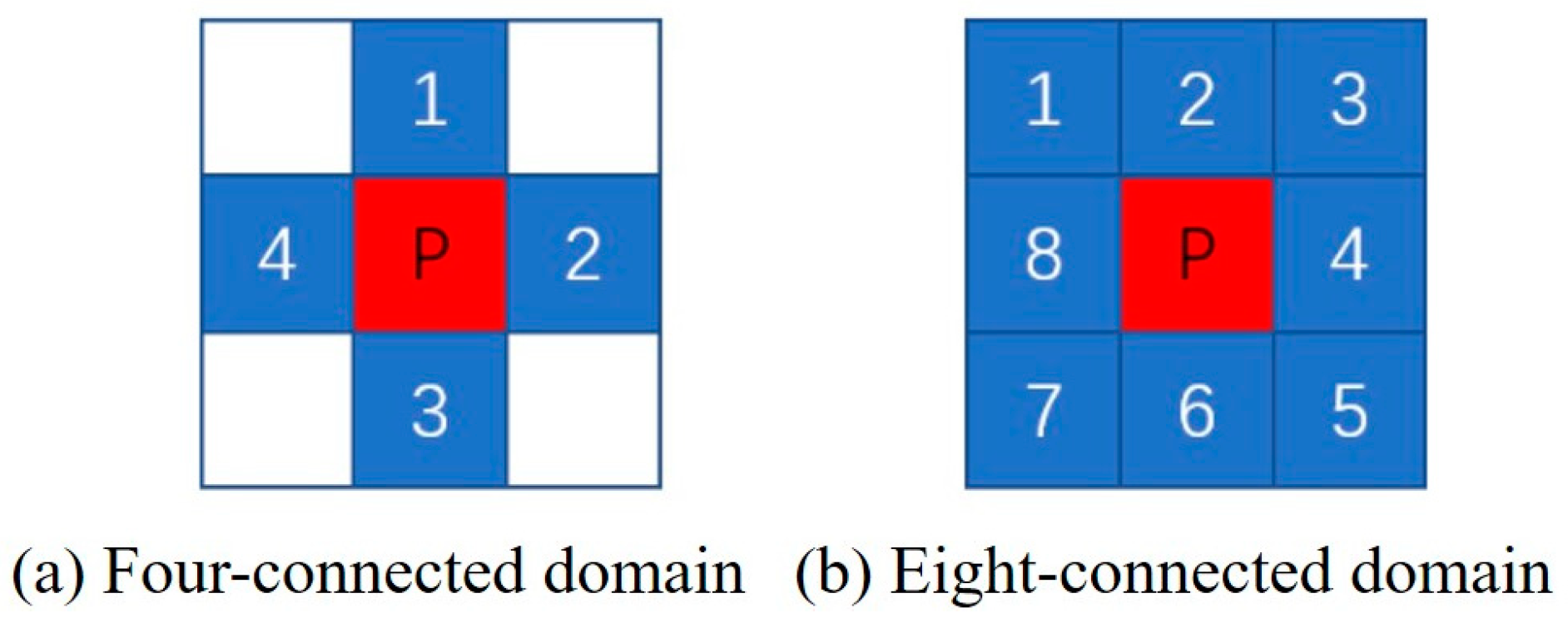
With (i, j) as the center and (i, j + 1) as the start point, find whether there exists a 1-pixel point in the connected domain of (i, j) in a clockwise direction. If it exists, let (p₁, q₁) be the first 1-pixel point in a clockwise direction; otherwise, continue scanning from point (i, j + 1) until the end of the bottom-right vertex of the image.

(d)

With (i, j) as the center and (p₁, q₁) as the start point, search counter-clockwise for the existence of a 1-pixel point in the connected domain of (i, j). If it exists, let (i, j) be B_k; if it is a pixel point that has already been checked, the scanning continues from the point (i, j + 1) until it ends at the bottom right vertex of the image.

(e)

Save the boundary topology sequence achieved from the above procedures as the extracted contours, then calculate and sort the areas of all the contours and take the largest one as the contour of the reference frame.

After extracting the contour points of the reference frame, the ApproxPolyDP [40] function was applied to fit polygons. The function is based on the Douglas–Peucker algorithm, which approximates the curve as a series of points. A straight line is first connected between the beginning and end points of the curve, then the largest distance between the point on the curve and the line is calculated. The distance is compared with a pre-given threshold. If the distance is smaller than the threshold, the straight-line segment will be used as an approximation of the curve; if the distance is larger than the threshold, the curve will be divided into two segments by the point, and then repeat the above operations for the two segments respectively. When all curves are processed, the fold lines formed by each segmentation point are connected sequentially.

The scale conversion between image pixels and the real-world millimeter-wise dimensions is realized by calculating the perimeter and area of the reference frame. In this study, the perimeter of a closed contour is calculated by the ArcLength function, which is able to count the length of the contour and return the value in pixels. The counted length is the distance of the line connecting two neighboring pixel points of the contour or the sum of all the line segments if the contour is closed. The area of the contour is calculated through the ContourArea function, which is based on Green’s formula. Assuming that the area D is enclosed by a segmented smooth curve L. The functions P(x, y) and Q(x, y) have first-order successive partial derivatives on D:

$${\displaystyle \underset{D}{\iint }(\frac{\partial Q}{\partial x}-\frac{\partial P}{\partial y})dxdy}={\displaystyle {\oint }_{L}Pdx+Qdy}$$

(6)

Knowing that the reference frame has a perimeter of 150 mm and an area of 1250 mm², the outline pixel-level perimeter is R_p and the pixel-level area is A_p, the real-world length and area conversion scales P_r, P_a of individual pixels are given as follows:

$$P_r={\displaystyle \frac{150}{R_p}},\hspace{1em}{P}_a={\displaystyle \frac{1250}{A_p}}$$

(7)

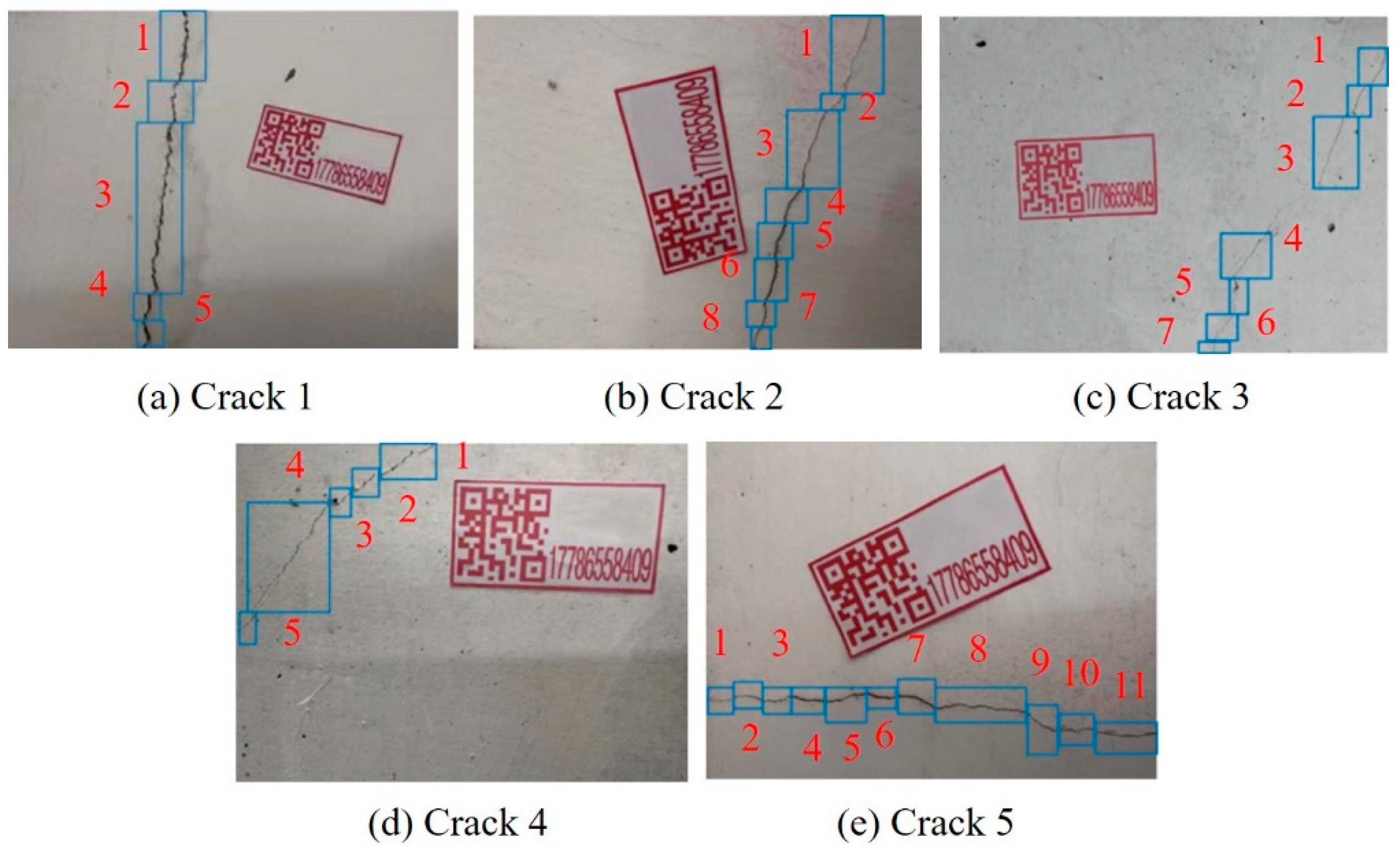
2.3. Millimeter-Wise Crack Dimensions Quantification (Step Three)

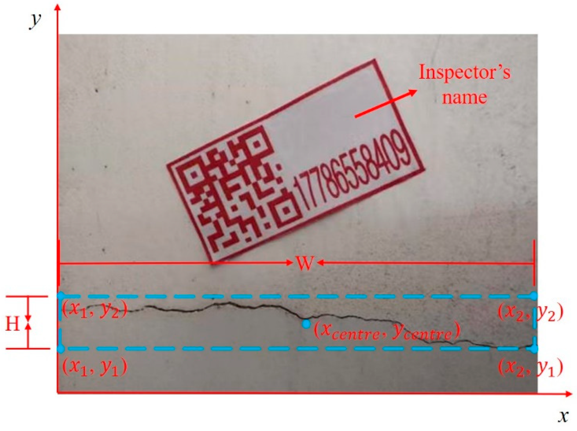
2.3.1. Target Bounding Box Cropping

In the previous section, the developed deep learning-based crack recognition algorithm uses a bounding box to localize the target. Therefore, the bounding box is firstly automatically cropped before extracting the contour of the concrete crack. The target information is saved to a file with a txt suffix after the crack recognition is completed, including the horizontal coordinate value x_centre of the target centroid, the vertical coordinate value y_centre of the target centroid, the width W of the target, and the height H of the target. As shown in Figure 5, it is necessary to obtain the coordinates of the four vertices, i.e., (x₁, y₁), (x₁, y₂), (x₂, y₁), and (x₂, y₂) to carry out the target bounding box cropping. Since target information stored in the txt file has been normalized, the original values of x₁, y₁, x₂, and y₂ must be multiplied by the width or height of the whole picture, which is calculated as Equation (8). Then, the box is cropped according to the four original values of x₁, y₁, x_2, and y₂ in the horizontal and vertical directions of the crack image, respectively.

$$\left\{\begin{array}{c}{x}_1=x_{centre}-{\displaystyle \frac{1}{2}}W,\hspace{1em}{y}_1=y_{centre}-{\displaystyle \frac{1}{2}}H\\ x_2=x_{centre}+{\displaystyle \frac{1}{2}}W,\hspace{1em}{y}_2=y_{centre}+{\displaystyle \frac{1}{2}}H\end{array}\right.$$

(8)

2.3.2. Crack Contour Extraction and Dimensions Quantification

After cropping the bounding box of the target, the FindContours algorithm is repeated to extract the complete contour of the crack. The ApproxPolyDP function to fit polygons to the contour points is also repeated. Then the pixel-wise perimeter and area of the crack are respectively calculated. Since the perimeter of the extracted contour is approximately twice that of the length, the pixel length is derived by dividing the perimeter by two in the actual calculation. According to the conversion scale obtained from the previous operation, the real-world length of the crack can be computed as follows:

$$L=P_r{R}_{crack}$$

(9)

where L refers to the crack length in mm, R_crack is the crack length in pixels, and P_r refers to the length conversion scale of individual pixels in mm/pixel.

The real-world damaged area of the crack can be computed as follows:

$$S=P_a{A}_{crack}$$

(10)

where S is the damaged area of the crack in mm², A_crack is the damaged area of the crack in pixels, and P_a is the area conversion scale of individual pixels in mm²/pixel.

The maximum width of the crack W_max is acquired by the maximum internal tangent circle algorithm, which is based on Canny edge detection and Hough transform [41]. After obtaining the crack edge image, the Houghcircle function is performed, and the parameters of the gradient threshold and the minimum distance from the center of the circle are adjusted. In the Hough transform, parameterized circles are used to represent circular edges, and the parameter space values corresponding to each combination of center and radius are computed, in which candidate values for the center and radius are stored in the accumulator. Finally, the circle with the largest radius, whose diameter is the maximum width of the crack, is indexed in the accumulator and can be computed as follows:

$$W_{\max }=P_r{D}_{crack}$$

(11)

where W refers to the maximum width of the crack in mm, D_crack is the diameter of the maximum internal tangent circle in pixels, and P_r refers to the length conversion scale of individual pixels in mm/pixel.

3. Experimental Procedures

3.1. Concrete Crack Recognition Model Training

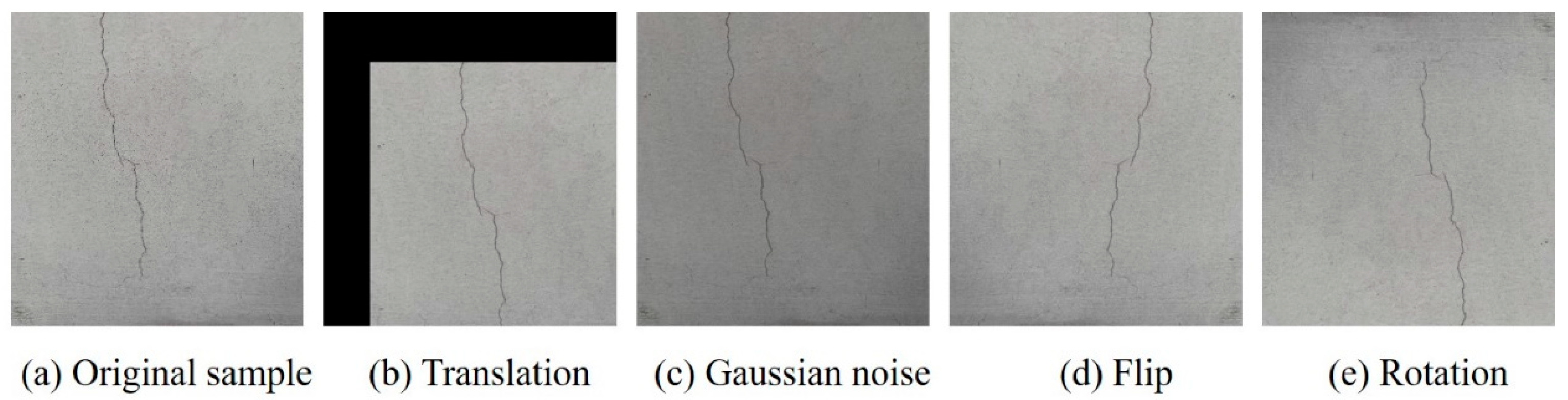
3.1.1. Setup of Image Datasets and Training Configurations

The image dataset created in this experiment was divided into two parts: damage images captured using smartphones during the process of infrastructure inspections and an open-source crack dataset collected from various campus buildings of the Middle East Technical University [42]. In order to improve the robustness of the proposed method, data augmentation was performed to avoid overfitting, and crack images were augmented by translation, Gaussian noise, flip, and rotation (Figure 6). Finally, a total of 4630 crack images were obtained and the training, validation, and test sets were partitioned by a ratio of 7:2:1. Feature labeling in the training set was carried out using the LabelMe graphical tool. The training experiment was conducted by applying deep learning for Python 3.8, Cudatoolkit 11.3.1, Cudnn 8.2.1, and Pytorch 1.12.1 on a computer with a Core i9-9900k @3.60 GHz CPU and a 11 GB NVIDIA GeForce RTX 2080Ti. At the beginning of training, the parameters were initialized to random values and normalized for each pixel value, allowing the results to converge faster. The value of the momentum optimizer was set to 0.937 in order to facilitate parameter updates between iterations. The optimizer was “SGD”, the learning rate was set to 0.01, and the weight of the network was set to decay to 0.0005. The batch size in this experiment was four, which contained multiple regions of interest in each iteration in order to evaluate the gradient of the loss function and update the weights. The number of epochs was 150, and the loss gain was set to 7.5, 0.5, and 1.5 for the bounding box, class, and DFL, respectively. The training of the crack recognition model took about 4 h in this experiment.

When tuning the training hyperparameters, Non-maximum suppression (NMS) was adopted to ensure that the algorithm gets only one detection box for each crack. In target detection, the model tends to propose a higher number of regions than the actual situation, which causes the output bounding boxes to be stacked (Figure 7a). NMS selects the bounding box with the highest confidence in each turn and then suppresses the remaining boxes that have a high overlap with the selected box. The bounding box selected in this turn will be retained in the output and will not appear in the next turn. The threshold of the IoU (area of overlap divided by area of union) was set to 0.8 in this study and the selecting process was repeated to finally output the optimum detecting box (Figure 7b).

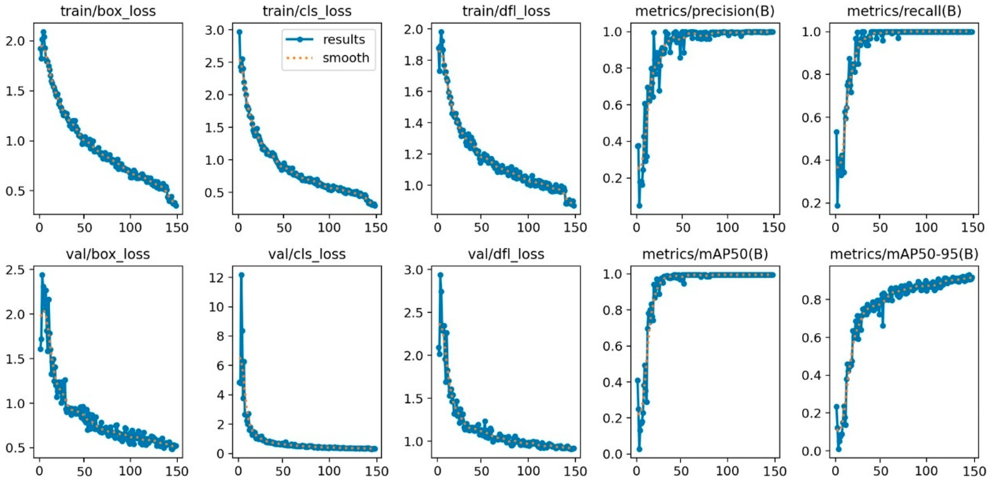
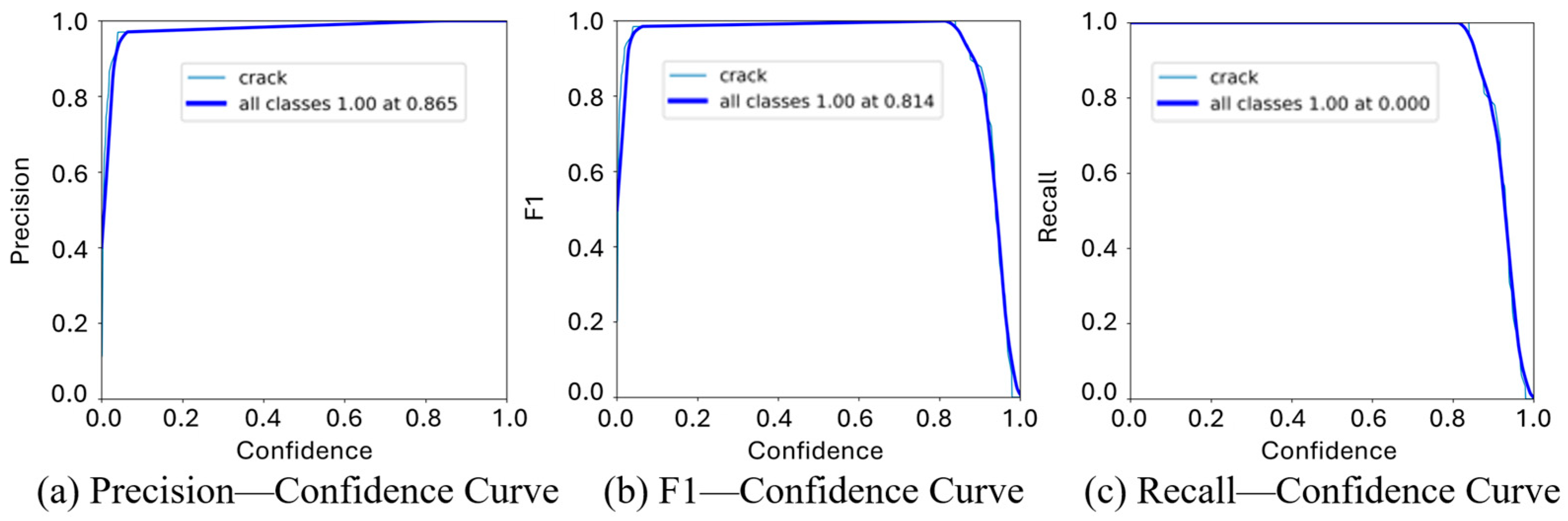
3.1.2. Indicator Analysis for Model Evaluation

In order to visualize the process of training and validation, the loss function was used to evaluate the performance of the detection model by measuring the deviation of its predicted and true values. The loss function includes a bounding box loss (box_loss), which refers to the error between the prediction box and the ground truth box; a classification loss (cls_loss), which calculates whether the anchor frame is correctly classified with the corresponding label; and a distribution focal loss (dfl_loss), which denotes the rectangular box regression error. The smaller value of the above losses represents the higher crack detection accuracy. Figure 8 shows the loss–epoch graph generated in the training and validation process of this experiment.

In addition, the metrics of precision (P) and recall (R) were adopted, and their functions are shown in Equations (12) and (13). There are four types of samples: true positive (TP), false positive (FP), true negative (TN), and false negative (FN). P was defined as the percentage of TP instances in all positive detection results, while R denoted the proportion of TP to the sum of TP and FN. The higher values of the precision and recall represent the better performance of the predicted model.

$$P={\displaystyle \frac{TP}{TP+FP}}$$

(12)

$$R={\displaystyle \frac{TP}{TP+FN}}$$

(13)

The F1 curve is defined as the harmonic mean of the precision and recall, which has a maximum of 1, as shown in Equation (14). Generally, when the confidence threshold is low, the samples with high recall and low precision are still considered to be true; when the confidence threshold is high, only samples with high confidence are considered to be true, and the more accurately the category is detected, the larger the precision value. Therefore, as can be seen in Figure 9b, the F1 scores at the beginning and end of the curve are smaller. The F1-Confidence curve obtained for 150 epochs indicates that it achieves relatively good scores in the confidence interval of 0.6–0.8.

$$F1=2\cdot {\displaystyle \frac{P\cdot R}{P+R}}$$

(14)

The precision–confidence curve shows the accuracy of each category (only crack in this experiment) recognition when the predicted probability exceeds the confidence threshold. When the confidence is higher, the category detection is more accurate, but it might also leave out some true samples with a lower probability of determination. For the recall–confidence curve, the smaller the confidence, the more comprehensive the category detection. Figure 10 displays some recognition examples on the test set, from which it can be seen that each crack on the image can be accurately detected. Results show that the average prediction accuracy of crack detection reaches up to 95.7% on the test dataset.

3.2. Crack Real-World Dimensions Identification

In order to verify the feasibility of the proposed fused IPTs-based crack dimensions identification method, five groups of crack images on the surface of concrete building structures were acquired and stamped with a pre-designed seal near the cracks as a reference frame for pixel scale conversion. Each group contained 60 image samples, and representative samples from each group of crack images were selected to calculate the relevant size parameters based on the pixel-to-millimeter conversion formula. Figure 11 demonstrates the process of quantifying the dimensions of the cracks for each set of representative samples, from which it can be seen that even cracks with smaller sizes can also be detected. The crack image was first input in the previously well-trained detection model, then converted into binary images to perform Gaussian filtering and Canny gradient algorithms. Subsequently, the seal contour was extracted by the FindContours algorithm to achieve the ratio between pixels and millimeter-wise sizes. In order to compare the crack dimensions obtained by the developed approach with the actual sizes, the width meter and vernier caliper were applied to measure the length and width of the crack. Since the development path of the crack is tortuous, it was divided into different segments according to the turning points (Figure 12). By measuring the length of each segment, its sum was taken as the actual length of the crack. At the same time, the width at the midpoint of each segment was measured and the maximum value was taken as the actual maximum width of the crack.

4. Result Analysis of Crack Quantification

The pixel length, pixel area, and conversion scale of each crack are shown in

Table 2. The pixel size and conversion scale of the cracks.

Crack No.	Length/Pixel	Area/Pixel	Length Conversion Scale	Area Conversion Scale
1	782.51	6084.90	0.2001	0.0404
2	719.55	6182.03	0.1468	0.0217
3	828.32	2053.18	0.1988	0.0393
4	644.34	3126.55	0.1342	0.0177
5	899.63	7034.25	0.1338	0.0181

. They were converted to achieve the millimeter-wise dimensions and compared with the length and maximum width obtained from the instrumental measurements. Since the seal and the crack are on the same image, and the extracted reference frame outlines are the pixel points in the outermost boundary of the seal, the conversion ratios achieved from this step do not have a significant effect on the quantification accuracy of the crack dimensions even though they differ on different crack images. The values of 60 samples of each group were then averaged to be the error coefficient, and the results are shown in

Table 3. Comparison of millimeter-wise dimensions quantification applied the proposed method and instrumental measurements for the cracks.

Crack No.	Quantitative Length/mm	Quantitative Area/mm2	Maximum Width/mm	True Length/mm	True Width/mm	Length Error/%	Width Error/%
1	156.58	245.83	1.77	167.50	1.83	6.52	3.28
2	105.63	134.15	1.47	112.25	1.52	5.90	3.29
3	164.67	80.69	0.70	155.90	0.65	5.63	7.69
4	86.47	55.34	0.84	82.60	0.78	4.69	7.33
5	120.37	127.32	1.26	124.05	1.30	2.97	3.08

. From Table 2 and Table 3, it can be seen that the real-world size information converted from the pixel dimensions is close to the true values obtained from the instrumental measurements, with the length error and the maximum width error within 7%.

When the width is greater than 1.0 mm, the error is smaller, basically within 4%; when the width is less than 1.0 mm, the error increases to about 8%. However, whether it is the length or the maximum width, the overall accuracy can still reach 90%, which means that the proposed method for quantifying the dimensions of concrete cracks can carry out accurate size conversion and performs well in crack detection. When defects such as pores are present on the concrete surface, the ArcLength function used in the proposed method filters them out and does not recognize them as cracks as it calculates the lengths of all closed contours and only returns the maximum value in pixels.

Although the accuracy of the proposed crack detection and quantification approach has been verified experimentally, the method still has some limitations. The first one is that the reference frame must be pre-stamped near the cracks since it is difficult to quantify the dimensions of the crack images based on the fused IPTs without a reference, which may lead to the limitation of the application and scenario scope. Secondly, when the background where the cracks are located is complex, the Gaussian filtering and Canny edge detection algorithms applied in the method require manual adjustment of the parameters and have differences in effects, so its robustness and generalization ability still need to be improved. Finally, the requirements of the actual crack dimensions identification are demanding (e.g., crack width detection is required up to a level of 0.5 mm). Therefore, the accuracy of the developed method needs to be further improved to meet the needs of building inspections in engineering projects.

5. Conclusions

In this paper, a three-step computer vision-based framework was proposed to quickly recognize concrete cracks and automatically quantify their dimensions millimeter-wise from damage images captured by a smartphone. In step one, the YOLOv8 object detection deep learning network is applied to train the model for recognizing the bounding box of each concrete crack in damage images; the average prediction accuracy for 463 test samples among 4630 crack images reached 95.7%. In step two, image processing technologies, including Gaussian filtering, Canny edge detection, and FindContours algorithms are integrated to extract contours of the reference frame in order to achieve the conversion scale between pixels and millimeter-wise sizes. The reference frame is a pre-designed seal that is stamped next to the crack and has a QR code on it, which aims to facilitate access to crack information by scanning and data recording for long-term inspection. In step three, the model trained in the first step is used to identify and crop the region of the crack, then the millimeter-wise crack length and area are computed due to the pixel ratio, as well as the maximum width obtained based on the maximum internal tangent circle algorithm. Results show that the precision of quantified crack dimensions is over 90% compared with the true values obtained from the instrumental measurements; the error increases as the crack size grows smaller (increasing to 8% when the crack width is within 1 mm).

Although the accuracy of the proposed method has been verified experimentally, it still has some limitations, such as the fact that the reference frame must be pre-stamped near the cracks in real cases, which may lead to the limitation of the application and scenario scope, such as bridges and culverts. When the background where the cracks are located is complex, the applied edge detection algorithms require manual adjustment of the parameters with variations in the results, resulting in inconvenience. Compared to the traditional method, the proposed method saves the time of measuring and recording the crack dimensions with an instrument but still requires more time to stamp the reference. In future work, more crack image data under various engineering environments will be trained to further improve the robustness of the proposed method. Additionally, in order to meet the requirements of the building inspections in actual engineering projects, the accuracy of the developed IPTs-based crack quantification algorithm should be improved. A relevant application program will also be studied and compiled, as well as attempts to use crawling robots to stamp seals to help engineers efficiently and portably detect cracks for on-site inspection and maintenance of concrete structures.

References

- Nishikawa, T.; Yoshida, J.; Sugiyama, T.; Fujino, Y. Concrete crack detection by multiple sequential image filtering. Comput.-Aided Civ. Infrastruct. Eng. 2012, 27, 29–47. [Google Scholar] [CrossRef]
- Qi, Y.; Yuan, C.; Kong, Q.; Xiong, B.; Li, P. A deep learning-based vision enhancement method for UAV assisted visual inspection of concrete cracks. Smart Struct. Syst. 2021, 27, 1031–1040. [Google Scholar]
- Dung, C.V. Autonomous concrete crack detection using deep fully convolutional neural network. Autom. Constr. 2019, 99, 52–58. [Google Scholar] [CrossRef]
- Shahrokhinasab, E.; Hosseinzadeh, N.; Monirabbasi, A.; Torkaman, S. Performance of image-based crack detection systems in concrete structures. J. Soft Comput. Civ. Eng. 2020, 4, 127–139. [Google Scholar]
- Hu, W.; Wang, W.; Ai, C.; Wang, J.; Wang, W.; Meng, X.; Liu, J.; Tao, H.; Qiu, S. Machine vision-based surface crack analysis for transportation infrastructure. Autom. Constr. 2021, 132, 103973. [Google Scholar] [CrossRef]
- Abdel-Qader, I.; Abudayyeh, O.; Kelly, M.E. Analysis of edge-detection techniques for crack identification in bridges. J. Comput. Civ. Eng. 2003, 17, 255–263. [Google Scholar] [CrossRef]
- Salman, M.; Mathavan, S.; Kamal, K.; Rahman, M. Pavement crack detection using the Gabor filter. In Proceedings of the 16th International IEEE Conference on Intelligent Transportation Systems (ITSC 2013), The Hague, The Netherlands, 6–9 October 2013; pp. 2039–2044. [Google Scholar]
- Kapela, R.; Śniata, P.; Turkot, A.; Rybarczyk, A.; Pożarycki, A.; Rydzewski, P.; Wyczalek, M.J.; Bloch, A. Asphalt surfaced pavement cracks detection based on histograms of oriented gradients. In Proceedings of the 2015 22nd International Conference Mixed Design of Integrated Circuits & Systems (MIXDES), Toruń, Poland, 25–27 June 2015; IEEE: New York, NY, USA, 2015; pp. 579–584. [Google Scholar]
- Quintana, M.; Torres, J.; Menéndez, J.M. A simplified computer vision system for road surface inspection and maintenance. IEEE Trans. Intell. Transp. Syst. 2015, 17, 608–619. [Google Scholar] [CrossRef]
- Varadharajan, S.; Jose, S.; Sharma, K.; Wander, L.; Mertz, C. Vision for road inspection. In Proceedings of the IEEE Winter Conference on Applications of Computer Vision, Steamboat Springs, CO, USA, 24–26 March 2014; IEEE: New York, NY, USA, 2014; pp. 115–122. [Google Scholar]
- Fadlullah, Z.M.; Tang, F.; Mao, B.; Kato, N.; Akashi, O.; Inoue, T.; Mizutani, K. State-of-the-art deep learning: Evolving machine intelligence toward tomorrow’s intelligent network traffic control systems. IEEE Commun. Surv. Tutor. 2017, 19, 2432–2455. [Google Scholar] [CrossRef]
- Bishop, C.M.; Nasrabadi, N.M. Pattern Recognition and Machine Learning; Springer: Berlin/Heidelberg, Germany, 2006; Volume 4. [Google Scholar]
- Rumelhart, D.E.; Hinton, G.E.; Williams, R.J. Learning representations by back-propagating errors. Nature 1986, 323, 533–536. [Google Scholar] [CrossRef]
- Dang, J.; Shrestha, A.; Haruta, D.; Tabata, Y.; Chun, P.; Okubo, K. Site verification tests for UAV bridge inspection and damage image detection based on deep learning. In Proceedings of the 7th World Conference on Structural Control and Monitoring, Qingdao, China, 22–25 July 2018. [Google Scholar]
- Kim, H.; Ahn, E.; Shin, M.; Sim, S.-H. Crack and noncrack classification from concrete surface images using machine learning. Struct. Health Monit. 2019, 18, 725–738. [Google Scholar] [CrossRef]
- Li, Y.; Li, H.; Wang, H. Pixel-wise crack detection using deep local pattern predictor for robot application. Sensors 2018, 18, 3042. [Google Scholar] [CrossRef] [PubMed]
- Da Silva, W.R.L.; de Lucena, D.S. Concrete cracks detection based on deep learning image classification. Multidiscip. Digit. Publ. Inst. Proc. 2018, 2, 489. [Google Scholar]
- Bang, S.; Park, S.; Kim, H.; Kim, H. A deep residual network with transfer learning for pixel-level road crack detection. In Proceedings of the International Symposium on Automation and Robotics in Construction, ISARC, Berlin, Germany, 20–25 July 2018; IAARC Publications: Berlin, Germany, 2018; Volume 35, pp. 1–4. [Google Scholar]
- Yeum, C.M.; Dyke, S.J.; Ramirez, J. Visual data classification in post-event building reconnaissance. Eng. Struct. 2018, 155, 16–24. [Google Scholar] [CrossRef]
- Elshafey, A.A.; Dawood, N.; Marzouk, H.; Haddara, M. Crack width in concrete using artificial neural networks. Eng. Struct. 2013, 52, 676–686. [Google Scholar] [CrossRef]
- Yamaguchi, T.; Hashimoto, S. Practical image measurement of crack width for real concrete structure. Electron. Commun. Jpn. 2009, 92, 1–12. [Google Scholar] [CrossRef]
- Cho, H.; Yoon, H.-J.; Jung, J.-Y. Image-based crack detection using crack width transform (CWT) algorithm. IEEE Access 2018, 6, 60100–60114. [Google Scholar] [CrossRef]
- Xu, X.; Zhao, M.; Shi, P.; Ren, R.; He, X.; Wei, X.; Yang, H. Crack detection and comparison study based on faster R-CNN and mask R-CNN. Sensors 2022, 22, 1215. [Google Scholar] [CrossRef] [PubMed]
- Attard, L.; Debono, C.J.; Valentino, G.; Di Castro, M.; Masi, A.; Scibile, L. Automatic crack detection using mask R-CNN. In Proceedings of the 2019 11th International Symposium on Image and Signal Processing and Analysis (ISPA), Dubrovnik, Croatia, 23–25 September 2019; IEEE: New York, NY, USA, 2019; pp. 152–157. [Google Scholar]
- He, K.; Gkioxari, G.; Dollár, P.; Girshick, R. Mask r-cnn. In Proceedings of the IEEE International Conference on Computer Vision, Venice, Italy, 22–29 October 2017; pp. 2961–2969. [Google Scholar]
- Liu, Z.; Cao, Y.; Wang, Y.; Wang, W. Computer vision-based concrete crack detection using U-net fully convolutional networks. Autom. Constr. 2019, 104, 129–139. [Google Scholar] [CrossRef]
- Redmon, J.; Divvala, S.; Girshick, R.; Farhadi, A. You Only Look Once: Unified, Real-Time Object Detection. In Proceedings of the 2016 IEEE Conference on Computer Vision and Pattern Recognition (CVPR), Las Vegas, NV, USA, 26 June–1 July 2016; IEEE: New York, NY, USA, 2016; pp. 779–788. [Google Scholar] [CrossRef]
- Nie, M.; Wang, C. Pavement Crack Detection based on yolo v3. In Proceedings of the 2019 2nd International Conference on Safety Produce Informatization (IICSPI), Chongqing, China, 28–30 November 2019; IEEE: Chengdu, China, 2019; pp. 327–330. [Google Scholar]
- Zhang, Y.; Huang, J.; Cai, F. On Bridge Surface Crack Detection Based on an Improved YOLO v3 Algorithm. IFAC-PapersOnLine 2020, 53, 8205–8210. [Google Scholar] [CrossRef]
- Park, S.E.; Eem, S.-H.; Jeon, H. Concrete crack detection and quantification using deep learning and structured light. Constr. Build. Mater. 2020, 252, 119096. [Google Scholar] [CrossRef]
- Shan, B.; Zheng, S.; Ou, J. A stereovision-based crack width detection approach for concrete surface assessment. KSCE J. Civ. Eng. 2016, 20, 803–812. [Google Scholar] [CrossRef]
- Yuan, C.; Xiong, B.; Li, X.; Sang, X.; Kong, Q. A novel intelligent inspection robot with deep stereo vision for three-dimensional concrete damage detection and quantification. Struct. Health Monit. 2022, 21, 788–802. [Google Scholar] [CrossRef]
- Hussain, M. YOLO-v1 to YOLO-v8, the rise of YOLO and its complementary nature toward digital manufacturing and industrial defect detection. Machines 2023, 11, 677. [Google Scholar] [CrossRef]
- Safie, S.I.; Kamal, N.S.A.; Yusof, E.M.M.; Tohid, M.Z.-W.M.; Jaafar, N.H. Comparison of SqueezeNet and DarkNet-53 based YOLO-V3 Performance for Beehive Intelligent Monitoring System. In Proceedings of the 2023 IEEE 13th Symposium on Computer Applications & Industrial Electronics (ISCAIE), Penang, Malaysia, 20–21 May 2023; IEEE: New York, NY, USA, 2023; pp. 62–65. [Google Scholar]
- Elfwing, S.; Uchibe, E.; Doya, K. Sigmoid-weighted linear units for neural network function approximation in reinforcement learning. Neural Netw. 2018, 107, 3–11. [Google Scholar] [CrossRef] [PubMed]
- Li, X.; Wang, W.; Wu, L.; Chen, S.; Hu, X.; Li, J.; Tang, J.; Yang, J. Generalized focal loss: Learning qualified and distributed bounding boxes for dense object detection. Adv. Neural Inf. Process. Syst. 2020, 33, 21002–21012. [Google Scholar]
- Ito, K.; Xiong, K. Gaussian filters for nonlinear filtering problems. IEEE Trans. Autom. Control. 2000, 45, 910–927. [Google Scholar] [CrossRef]
- Samanta, S.; Pal, M. Fuzzy Threshold Graphs. CiiT Int. J. Fuzzy Syst. 2011, 3, 360–364. [Google Scholar]
- Manuaba, P.; Indah, K.A.T. The object detection system of balinese script on traditional Balinese manuscript with findcontours method. Matrix J. Manaj. Teknol. Dan Inform. 2021, 11, 177–184. [Google Scholar] [CrossRef]
- Gervasi, O.; Caprini, L.; Maccherani, G. Virtual exhibitions on the web: From a 2d map to the virtual world. In Proceedings of the Computational Science and Its Applications. ICCSA 2013: 13th International Conference, Ho Chi Minh City, Vietnam, 24–27 June 2013; Proceedings, Part I 13. Springer: Berlin/Heidelberg, Germany, 2013; pp. 708–722. [Google Scholar]
- Illingworth, J.; Kittler, J. A Survey of the Hough Transform. Comput. Vis. Graph. Image Process. 1988, 44, 30. [Google Scholar] [CrossRef]
- Özgenel, Ç.F. Concrete Crack Images for Classification, Version 2. 2019. Available online: https://data.mendeley.com/datasets/5y9wdsg2zt/2 (accessed on 23 June 2024).