Contribution and Marginal Effects of Landscape Patterns on Thermal Environment: A Study Based on the BRT Model

Abstract

Urban landscape patterns significantly impact land surface temperature (LST) and the urban heat island (UHI) effect. This study employs the boosted regression tree (BRT) model and variance partitioning analysis to examine the contributions and relationships of two-dimensional and three-dimensional building and vegetation patterns to LST, and their marginal effects at different heights. The results show that the dominant indicators affecting LST differ between buildings and vegetation, with three-dimensional building features being slightly more important than two-dimensional features (percentage of landscape of buildings) and two-dimensional vegetation features (three-dimensional green index) having a greater impact than three-dimensional features. When both buildings and vegetation are considered, building patterns still have significant explanatory power. Building height differences influence each indicator’s contribution and marginal effects on LST, with lower-height areas seeing a joint dominance of buildings and vegetation on LST changes, and higher-height areas showing greater impact from vegetation indicators. Increasing the percentage of landscape of vegetation (PLAND_V) provides the best cooling effect in lower-building-height areas, but in higher-building-height areas, the cooling effect weakens, requiring additional vegetation indicators to assist in cooling.

1. Introduction

In 2019, the Intergovernmental Panel on Climate Change (IPCC), in its special report on the impacts of global warming of 1.5 °C above pre-industrial levels and related global greenhouse gas emission pathways, stated: “Human activities are estimated to have caused approximately 1.0 °C of global warming above pre-industrial levels… Global warming is likely to reach 1.5 °C between 2030 and 2052 if it continues to increase at the current rate (high confidence)” [1]. The heat island effect, UHI, is specifically defined as the phenomenon in which urban temperatures are warmer than those in the surrounding suburban and rural areas [2]. The urban heat island (UHI) effect is a typical urban problem globally [3]. The intensification of the UHI effect has severely threatened the living environment and health of urban residents as well as the flora and fauna living in cities [4], with urban challenges increasing daily. Therefore, it is of significant reference value and practical significance for urban planners and policymakers to thoroughly explore the relationship between the UHI effect and related influencing factors. Urban land surface temperature (ULST) is a key surface characterization parameter in urban heat island research [5].

Landscape patterns refer to the spatial distribution of land cover types and the proportion of each landscape type [6]. These are manifested explicitly as the spatial forms of buildings, vegetation, water bodies, etc., in terms of their area, height, and spatial configuration. Numerous studies have shown that the spatial form of urban landscapes plays a significant role in changes to land surface temperature (LST) [7,8,9]. Currently, domestic and international researchers mainly use landscape metrics to quantify the impact of landscape patterns on LST. For example, Chen et al. [10] calculated traditional two-dimensional characteristic indicators (such as patch area, edge density, etc.) to explore their correlation with LST, proving that percentage composition of landscape (PLAND), largest patch index (LPI), division index (DIVISION), percentage of like adjacencies (PLADJ), and the Interspersion and Juxtaposition Index (IJI) are indices that exhibit stable significant correlations in the analysis of major urban landscape types (forests, buildings) and LST. Yun et al. [11] used the Patch Cohesion Index (COHESION), Landscape Division Index (DIVISION), effective mesh size (MESH), area index (AI), and other two-dimensional morphological indices to quantitatively study the response mechanisms and parameter curves of urban morphology layout and UHI intensity, finding that UHI intensity increases with urban morphology area, with a linear relationship between patch area and maximum UHI increase for patches over 50 km², and a quadratic curve relationship with total UHI increase. Zhou, Huang, and other scholars [12] studied and calculated various two-dimensional landscape indices for buildings, green spaces, and water bodies, finding that the most influential land cover characteristic affecting LST magnitude was the percentage cover of buildings.

Despite the substantial achievements of current research, there are still limitations. Previous studies mainly focused on the relationship between urban landscape types such as buildings and vegetation and LST from the perspective of traditional two-dimensional landscape patterns. However, as cities increasingly expand vertically, the complexity of urban composition and patterns increases. Therefore, some studies have found that the vertical structure of high-rise buildings significantly impacts the urban thermal environment [13,14,15]. In this context, explaining the relationship between urban landscape patterns and the thermal environment from only a two-dimensional perspective can no longer meet the needs of current urban thermal environment research. In recent years, scholars have gradually attempted to explore the relationship between urban three-dimensional landscape patterns and the thermal environment. For example, at the urban agglomeration scale, Yu et al. [13] explored the impact of three-dimensional building morphology (nine indicators) on LST, finding that the building structure index (BSI), average building volume (AV), and building evenness index (BEI) had the most significant effects on LST; at the city scale, Guo et al. [14] used a set of three-dimensional landscape metrics based on landscape composition and structure to study their spatiotemporal relationship with LST in Beijing’s old city, finding that denser and more compact building patterns lead to higher diurnal land surface temperatures (DLSTs) and three-dimensional landscape metrics were significantly correlated with DLSTs. Some scholars have also studied the relationship between different types of street block layouts and the thermal environment at the street block scale, such as Jiang et al. [15], who studied the relationship between different spatial element combinations and the thermal environment in residential areas, comparing the ecological and energy-saving effects of different element combination modes from the perspectives of the overall three-dimensional spatial composition of the residential regions, building morphology, and green morphology, proving that building morphology has a more significant impact on the residential area’s thermal environment compared to green morphology.

However, since both two-dimensional and three-dimensional patterns are essential features of urban landscape patterns and both affect the urban thermal environment, some scholars believe that it is not comprehensive to consider only the relationship between urban two-dimensional patterns or three-dimensional patterns and the thermal environment. Based on this, some scholars have begun to simultaneously assess the impact of two-dimensional and three-dimensional landscape patterns on the thermal environment. For instance, Srivanit et al. [16] systematically analyzed the relationship between 12 two-dimensional and three-dimensional urban pattern metrics and LST and air temperature, finding that three-dimensional pattern metrics had a more significant impact on LST; Xu et al. [17] used the BRT model to analyze the relationship and seasonal differences between two-dimensional and three-dimensional urban patterns and LST in three cities of different scales. The results show that in summer, LST gradually increases with city size (Cangzhou < Shijiazhuang < Beijing), while in winter, LST gradually decreases with city size (Cangzhou > Shijiazhuang > Beijing). Some scholars have also discussed the spatial effects of two-dimensional and three-dimensional built environments on LST in cities with different terrains [18]. These studies collectively show that urban patterns containing vertical (three-dimensional) information can also respond to LST changes, sometimes having a more significant impact on LST than horizontal (two-dimensional) patterns.

In summary, it can be seen that changes in the two-dimensional landscape pattern (e.g., area of buildings, vegetation, etc.) can significantly affect the surface heat storage capacity, and thus, the intensity of the urban heat island effect. At the same time, changes in three-dimensional landscape patterns (building, vegetation height and volume, and other indicators) can not only change the degree of solar radiation absorption, but also affect the natural ventilation of the city, which ultimately leads to different urban heat. Methodologically, scholars have gradually begun to use the BRT model, which can significantly improve the stability and prediction accuracy, to predict the specific impact thresholds of the landscape pattern on the thermal environment, which will more intuitively show the extent of the impact of the landscape pattern. To illustrate, an in-depth exploration of the correlation between 2D and 3D urban landscape patterns and LST will provide a more accurate and comprehensive access to the mechanism of urban landscape patterns on UHI, which will help policymakers and designers to mitigate the UHI effect through rational urban planning. However, due to the limitations of data acquisition and representation capabilities for three-dimensional data, current research on urban three-dimensional landscape patterns is mainly concentrated on the construction of three-dimensional characteristics, pattern metrics, and pattern characteristic descriptions at the preliminary stage. There is still a lack of specific impact effect values (marginal effects) for various landscape pattern metrics. Research on urban three-dimensional landscape patterns is still in the exploratory and development stages. On the other hand, most studies have only provided intuitive references on the impact of three-dimensional buildings on LST, with almost no consideration of three-dimensional vegetation in cities. As vegetation (trees) is an integral part of the urban three-dimensional landscape pattern, it significantly impacts the urban thermal environment [19].

Suzhou is a rapidly developing city in eastern China, and its building pattern has changed significantly with the process of urbanization. Its complex building pattern is an ideal laboratory to study the surface temperature under different landscape patterns. And with the frequent occurrence of extreme weather in Suzhou in recent years, it is important to explore the landscape indicators that dominate the change in LST to improve the urban thermal environment. Therefore, exploring the landscape metrics that dominate LST changes and their specific impact thresholds has significant practical value for urban planning and renovation. Based on this, this study comprehensively considers the two-dimensional and three-dimensional pattern characteristics of buildings and vegetation, using high-resolution remote sensing satellite GF-2 images and the BRT model to explore the separate and combined contributions of two-dimensional and three-dimensional landscape patterns of buildings and vegetation to LST in Suzhou, identifying the landscape metrics that dominate LST changes. It also evaluates the specific impact and threshold of two-dimensional and three-dimensional landscape pattern metrics on LST in different building height scenarios to provide references and suggestions for adjusting various landscape component metrics and reasonably improving the urban thermal environment in different building height areas.

2. Materials and Methods

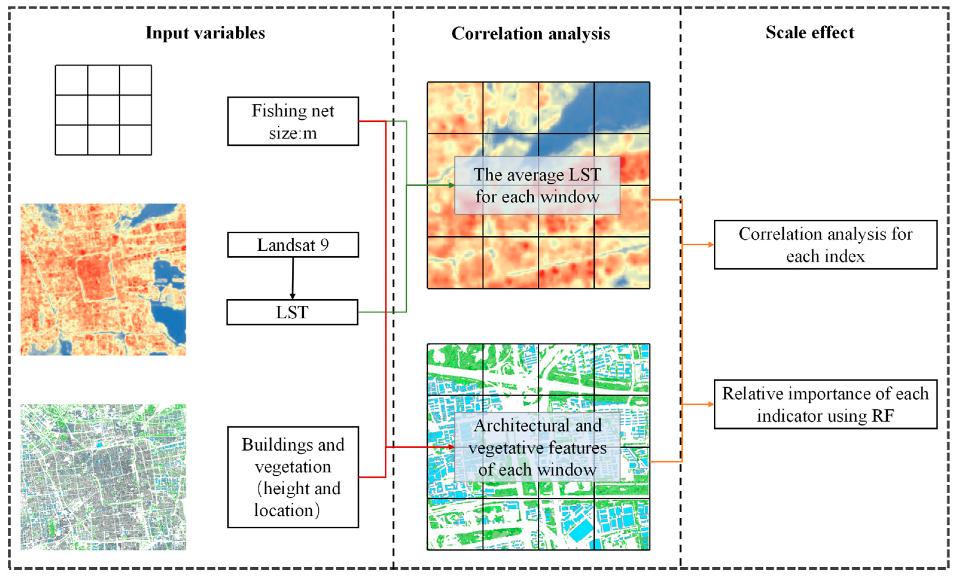
2.1. Overall Technical Approach

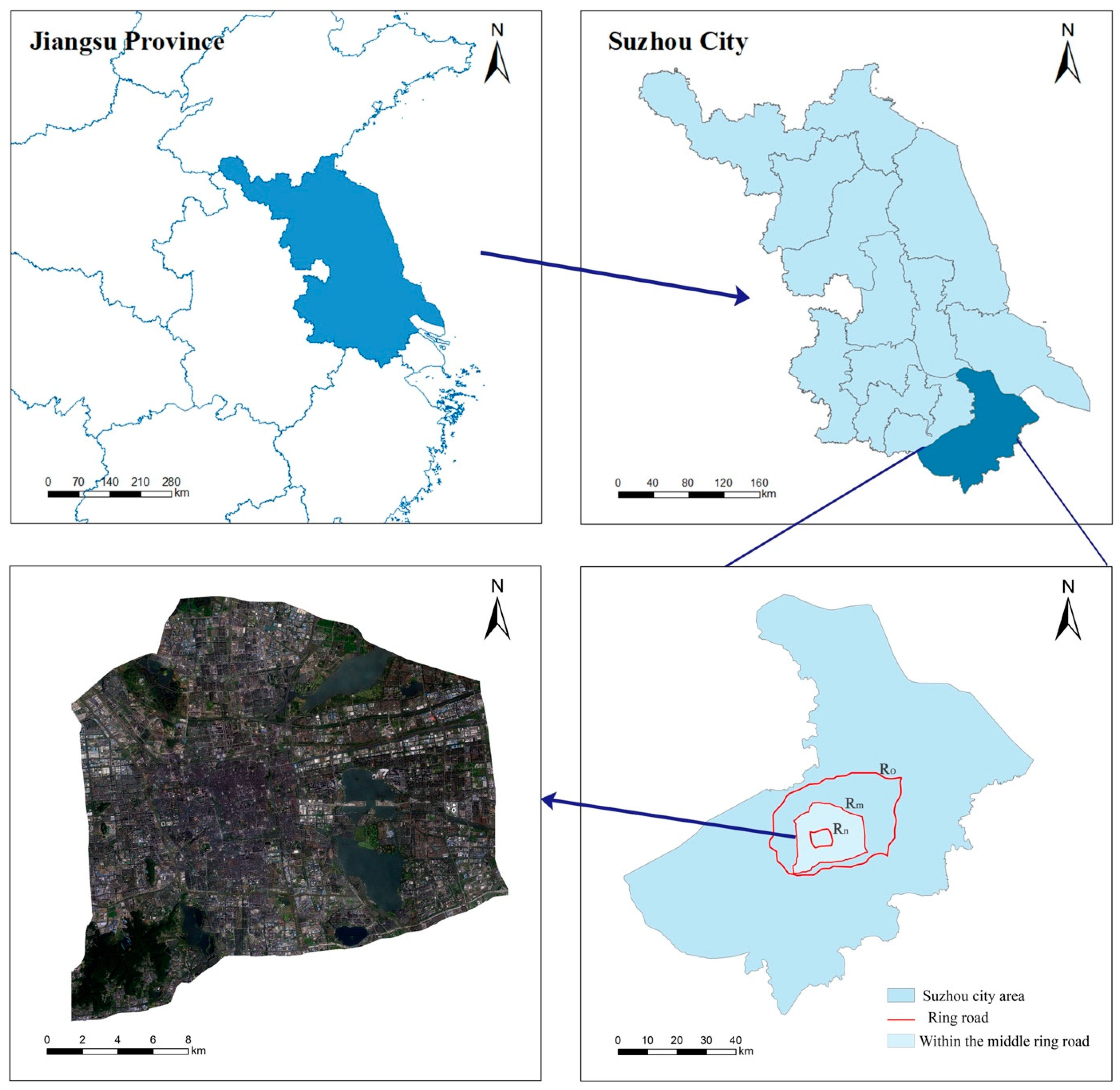
The overall technical approach of this study is shown in Figure 1. This study uses remote sensing data and auxiliary data containing building height information to extract LST and various indicator information. We construct a landscape metrics system, including two-dimensional indicators, three-dimensional indicators, building indicators, and vegetation indicators. We conduct statistical analysis based on these indicator values: using the BRT model for training, selecting dominant indicators for correlation analysis and contribution calculation, and predicting marginal effect values.

2.2. Study Area

Suzhou City is located in Jiangsu Province, China, and is one of the important central cities in the Yangtze River Delta. Suzhou has a subtropical monsoon maritime climate, with an average annual temperature of 18.1 °C and an average annual precipitation of 1086.3 mm. With urbanization, the population of Suzhou exceeded 5 million by 2022, making it a megacity.

As one of the first cities listed in the historical and cultural directory, Suzhou’s old city area contains many traditional buildings, including the Pingjiang Historical Block, characterized by low building heights and high distribution density. During the construction of the new city, Suzhou’s building patterns underwent significant changes, introducing numerous mid- and high-rise buildings both within and outside the old city. Traditional low-rise residences and modern mid- to high-rise buildings form Suzhou’s multi-architectural landscape. In addition to the old city’s modern residential areas, consisting mainly of mid- and high-rise buildings with moderate density, the Suzhou Industrial Park and some central business districts also feature high-rise buildings with a relatively scattered distribution. Suzhou’s complex building patterns provide ideal samples for studying the relationship between different building landscape spatial patterns and LST.

The sample area selected for this study is concentrated within Suzhou’s Middle Ring Road, as shown in Figure 2. The Middle Ring Road area includes the entire old city area of Suzhou—Gusu District; parts of Xiangcheng District, Huqiu District, Wuzhong District, and the Industrial Park.

2.3. Data and Preprocessing

The data used in this study include satellite data for retrieving LST, high-resolution remote sensing data for extracting vegetation areas and vegetation shadows, and urban building height data, as detailed in

Table 1. Dataset and descriptions.

Data	Type	Source
Remote sensing images	Raster data (0.8 m)	GF-2
LST data	Raster data (100 m)	Landsat 9 OLI/TIRS
Building height data	Vector data	Baidumap

.

The selected satellite remote sensing data are Landsat 9 data from 7 August 2022, for Suzhou, from which LST data were calculated. The GF-2 remote sensing image from 12 October 2021 was used to extract vegetation areas and vegetation shadows. This image underwent preprocessing (radiometric correction, atmospheric correction, orthorectification, and image fusion) in the ENVI 5.6 software, resulting in final image data with a resolution of 0.8 m. Additionally, since building height data cannot be directly obtained, this study used building floor data from Baidu Maps, multiplying the number of floors by 3 m to produce building height vector data. The overall accuracy of building heights obtained by this method can reach 86.78% [20], and due to the regularity of buildings in each city, this approximation is acceptable [21].

A study area grid with a 500 m × 500 m fishnet was constructed for this study. Subsequently, each grid cell contained a set of landscape pattern indices and corresponding LST values for statistical analysis (Figure 3).

2.4. Indicator Construction

This study uses landscape metrics to quantify buildings’ and vegetation’s two-dimensional and three-dimensional characteristics. Based on previous research, we selected four typical two-dimensional landscape indices, as shown in

Table 2. Selected landscape pattern metrics in the study.

Landscape Metrics	Abbreviation	Category	Formula	Description
Percentage of landscape	PLAND, %	2D	${\displaystyle \frac{\sum \mathrm{F}}{\mathrm{A}}}$	F: The land area of building/vegetation (m2) A: Study area (m2)
Edge density	ED	2D	${\displaystyle \frac{{\sum }_{\mathrm{i}-1}^{\mathrm{n}}{\mathrm{e}}_{\mathrm{j}}}{\mathrm{A}}}$	n: Number of patches within the statistical unit ej: Total edge length of building/vegetation patches
Patch density	PD	2D	${\displaystyle \frac{{\mathrm{n}}_{\mathrm{i}}}{\mathrm{A}}}\times 1000\times 100\mathrm{\%}$	ni: Number of patches
Landscape shape index	LSI	2D	${\displaystyle \frac{{\mathrm{e}}_{\mathrm{j}}}{\mathrm{m}\mathrm{i}\mathrm{n} {\mathrm{e}}_{\mathrm{j}}}}$	ej: Total edge length of building/vegetation patches min ej: Minimum total length of the edge in each patch
Mean architecture/vegetation height	MAH/MVH, m	3D	${\displaystyle \frac{\sum _{\mathrm{i}-1}^{\mathrm{n}}{\mathrm{H}}_{\mathrm{i}}}{\mathrm{N}}}$	Hi: Architecture/vegetation height
Mean architecture height standard deviation	AHSD/ VHSD, m	3D	$\sqrt{{\displaystyle \frac{\sum _{\mathrm{i}-1}^{\mathrm{n}}{\left({\mathrm{H}}_{\mathrm{i}}-\mathrm{M}\mathrm{H}\right)}^2}{\mathrm{N}}}}$	MH: Mean architecture/vegetation height (m)
Floor area ratio	FAR, %	3D	${\displaystyle \frac{\sum _{\mathrm{i}=1}^{\mathrm{n}}\left(\mathrm{C}\times \mathrm{F}\right)}{\mathrm{A}}}$	C: Number of floors
Building volume	BV	3D	${\displaystyle \sum _{\mathrm{i}-1}^{\mathrm{n}}}{\mathrm{F}}_{\mathrm{i}}\times {\mathrm{H}}_{\mathrm{i}}$	Fi: The land area of building (m2) Hi: Architecture/vegetation height
Three-dimensional green index	TGI	3D	${\displaystyle \frac{\sum {\mathrm{C}}_{\mathrm{i}}{\mathrm{S}}_{\mathrm{i}}}{\mathrm{A}}}$	Ci: Height level corresponding to the i-th vegetation pixel in the study area Si: Actual area corresponding to the i-th vegetation pixel (m2) ∑ Ci Si: Equivalent base green vegetation area
Shannon’s diversity index	SHDI	3D	${\displaystyle \sum _{\mathrm{i}=1}^{\mathrm{N}}}{\mathrm{P}}_{\mathrm{i}}\times \mathrm{l}\mathrm{n}{\mathrm{P}}_{\mathrm{i}}$	Pi: The proportion of the landscape occupied by patch type i
Sky view factor	SVF	3D	$1-{\displaystyle \frac{\sum _{\mathrm{i}=1}^{\mathrm{n}}\sin {\mathsf{\gamma }}_{\mathrm{i}}}{\mathrm{n}}}$	n: Number of calculated azimuth angles
Normalized 3D compactness index	NVCI	3D	${\displaystyle \frac{{\mathrm{Q}}^{\prime }\left({\mathrm{Q}}^{\prime }-1\right)}{\mathrm{N}\left(\mathrm{N}-1\right)}}\times {\displaystyle \frac{\sum \frac{{\mathrm{V}}_{\mathrm{i}}{\mathrm{V}}_{\mathrm{j}}}{{\mathrm{d}}^2\left(\mathrm{i},\mathrm{j}\right)}}{\sum \frac{{{\mathrm{V}}^{\mathrm{i}}}_{{\mathrm{i}}^{\prime }}{{\mathrm{V}}^{\prime }}_{{\mathrm{j}}^{\prime }}}{{\mathrm{d}}^{\prime 2}\left({\mathrm{i}}^{\prime },{\mathrm{j}}^{\prime }\right)}}}$	d(i,j): The geometric distance between centroids of urban cube i and cube j d(i′,j′): The distance between cube i′ and j′ Vi and Vj: The volume of urban buildings in urban cube i and cube j Vi′ and Vj′: The volumes of the equivalent spheres in cubes i′ and j′ Q′: The total number of cubes which the equivalent sphere occupies N: The number of all cubes

. For urban two-dimensional vegetation indicators, we used an object-oriented classification method to identify and extract vegetation areas within the study area, calculating patch area, perimeter, and density.

The three-dimensional indicators selected in this study (Table 2) represent urban three-dimensional building patterns from the perspectives of height, volume, and visible sky area [22]. Building heights are categorized into four classes: 0–10 m, 10–20 m, 20–35 m, and >35 m. Vegetation heights are classified into five classes: <1 m, 1–3 m, 3–6 m, 6–10 m, and >10 m, and the Shannon diversity index for building height (SHDI_B) and vegetation height (SHDI_V) is calculated for each class. Vegetation height classification is based on the urban vegetation vertical cooling effect reported by Alexander et al. (1 m, 1.0 °C; 3 m, 2.5 °C; 6 m, 4.5 °C; 10 m, 5.5 °C) [23].

This study introduces a new normalized urban compactness index constructed by Hu et al. [24], which considers multiple factors, including building height, building density, street layout, and open space. This comprehensive compactness index was calculated using Python. First, the location, area, and height data of buildings were obtained. Buildings were then considered as volumes in three-dimensional space, and the total volume of all buildings was compared to the total volume of the study area to derive the three-dimensional compactness index. The closer the NVCI value is to 1, the more compact the urban spatial form.

Other indicators were calculated using Fragstats 4.2 and ArcGIS 10.0 zonal statistics functions and are visualized as raster heat maps.

2.5. Vegetation Height Retrieval

This study uses a method developed by Bai et al. [25] for quickly measuring urban-scale green landscapes using high-resolution (GF-2) images. This method not only saves substantial field measurement costs but also has an average absolute error of less than 1 m [25], within the allowable error range for vegetation height classification (3 m). Therefore, using the formula, this method was chosen to extract vegetation shadows and retrieve vegetation height information.

Using 0.8 m resolution GF-2 remote sensing images, we employed the object-oriented classification software eCognition 9.0 [26], based on multi-scale segmentation algorithms and spectral difference algorithms, to extract shadow information, vegetation information, and water body information. First, based on the specific conditions of the study area image, we selected a segmentation layer with a scale of 120 to extract coarse-scale shadows and water bodies, including building shadows. Next, we distinguished the two based on brightness, area, and NDWI characteristics. After removing building shadows and water bodies, fine-scale shadows were further extracted. Finally, a segmentation layer with a scale of 30 was selected to extract grassland and forest land, distinguishing between the two based on homogeneity and NDVI values. We removed the vegetation shadows on the buildings as outliers and replaced them with the length of nearby similar shadow patches.

Based on the extracted information, the neighborhood analysis function in ArcGIS was used to extract vegetation shadows from fine-scale shadows. Then, the corresponding shadow length of the vegetation was calculated using the geometric relationship formula of the sun, satellite, and tree shadow positions. The calculation formula is as follows:

$$\mathrm{H}=\mathrm{A}{·\left({\tan }^{-2}\mathsf{\beta }+{\tan }^{-2}\mathsf{\alpha }-2{\tan }^{-1}\mathsf{\beta }·{\tan }^{-1}\mathsf{\alpha }·\cos \mathsf{\gamma }\right)}^{-{\displaystyle \frac{1}{2}}}$$

(1)

where H is the vegetation height, A is the actual shadow length of the corresponding vegetation area, and α, β, and γ are the satellite elevation angle (°), solar elevation angle (°), and the angle between the solar and satellite azimuth (°), respectively.

The retrieved vegetation height results are shown in Figure 4 (partial).

2.6. Land Surface Temperature Retrieval

This study retrieved land surface temperature (LST) using Landsat 9 data. Using a specific formula, the radiative transfer equation (RTE) method was employed to calculate the land surface emissivity (ε). Using the Band Math tool, the blackbody radiation radiance value (B(TS)) was calculated by combining the land surface emissivity and thermal infrared band data. The formula is as follows:

$$\mathrm{L}\mathsf{\lambda }=[\mathsf{\epsilon }\times \mathrm{B}(\mathrm{T}\mathrm{S})+(1-\mathsf{\epsilon })\times \mathrm{L}\downarrow ]\times \mathsf{\tau }+\mathrm{L}\uparrow 45$$

(2)

where Lλ is the received thermal infrared radiation radiance value, L↓ is the atmospheric downward radiance, τ is the atmospheric transmissivity, and L↑ is the atmospheric upward radiance. The blackbody radiation radiance value B(TS) is calculated as follows:

$$\mathrm{B}\left(\mathrm{T}\mathrm{S}\right)=[\mathrm{L}\mathsf{\lambda }-\mathrm{L}\uparrow -\mathsf{\tau }\times (1-\mathsf{\epsilon })\times \mathrm{L}\downarrow ]/(\mathsf{\epsilon }\times \mathsf{\tau })$$

(3)

Finally, the land surface temperature (TS) is calculated using Planck’s formula and converted from kelvin (K) to Celsius (°C) as follows:

$$\mathrm{T}\mathrm{S}=\mathrm{K}2/\mathrm{l}\mathrm{n}(\mathrm{K}1/\mathrm{B}(\mathrm{T}\mathrm{S})+1)\times 4$$

(4)

2.7. Sample Division and Classification

Four scenarios were set up based on the characteristics of Suzhou’s buildings. Within the Middle Ring area, building heights were classified according to the Unified Standard for Civil Building Design into four height scenarios: BH₁: 0–10 m, BH₂: 10–20 m, BH₃: 20–35 m, and BH₄: >35 m. The sample grid classifications for the four scenarios based on MAH values are shown in Figure 5. The sample sizes are 624, 596, 219, and 100, respectively (

Table 3. Classification criteria and sample size.

Scenario	Description	Sample Size
BH1	<10 m	624
BH2	10–20 m	596
BH3	20–35 m	219
BH4	>35 m	100

).

2.8. Statistical Analysis

2.8.1. Boosted Regression Tree (BRT) Model

The BRT model was chosen to select relatively important landscape metrics and predict their marginal effects on LST in specific samples. The BRT machine learning algorithm is widely used in predicting the impact of urban landscapes on LST [27,28] and is a popular ensemble learning algorithm [29]. It can handle various types of data, including classification and regression problems, as well as nonlinear and interactive effects. Due to its ability to sensitively capture nonlinear relationships between variables and its excellent predictive ability, it has been widely used in environmental and ecological research [30,31].

This study used two-dimensional and three-dimensional urban landscape metrics (PLAND_B, PLAND_V, LSI_B, LSI_V, ED_B, ED_V, PD_B, PD_V, MAH, MVH, AHSD, VHSD, FAR, BV, TGI, SHDI_B, SHDI_V, SVF, NVCI) and LST as independent and dependent variables, respectively, using the “gbm” package in RStudio 4.3.0.

First, the BRT model was used to evaluate the relative importance of each metric on LST when considering only building impacts or vegetation impacts. Then, the relative importance of all metrics on LST was evaluated when considering both building and vegetation impacts. Next, based on the characteristics of Suzhou’s building patterns, the relative importance was evaluated under the four scenarios BH₁, BH₂, BH₃, and BH₄, with sample sizes of 624, 596, 219, and 100, respectively. Subsequently, the marginal effects of the top five contributing metrics for each scenario were analyzed.

2.8.2. Variance Partitioning Analysis

Variance partitioning generates the proportion of variance for each component, which can be used to quantify the relative contribution of different effects to the total variation [32]. This method can determine the contribution of different categories of landscape metrics to LST. The metric categories in this study were divided into two-dimensional and three-dimensional metrics and building and vegetation metrics, resulting in four categories: two-dimensional building metrics, three-dimensional building metrics, two-dimensional vegetation metrics, and three-dimensional vegetation metrics. Variance partitioning was used to determine the explanatory power of these four categories on LST.

3. Results

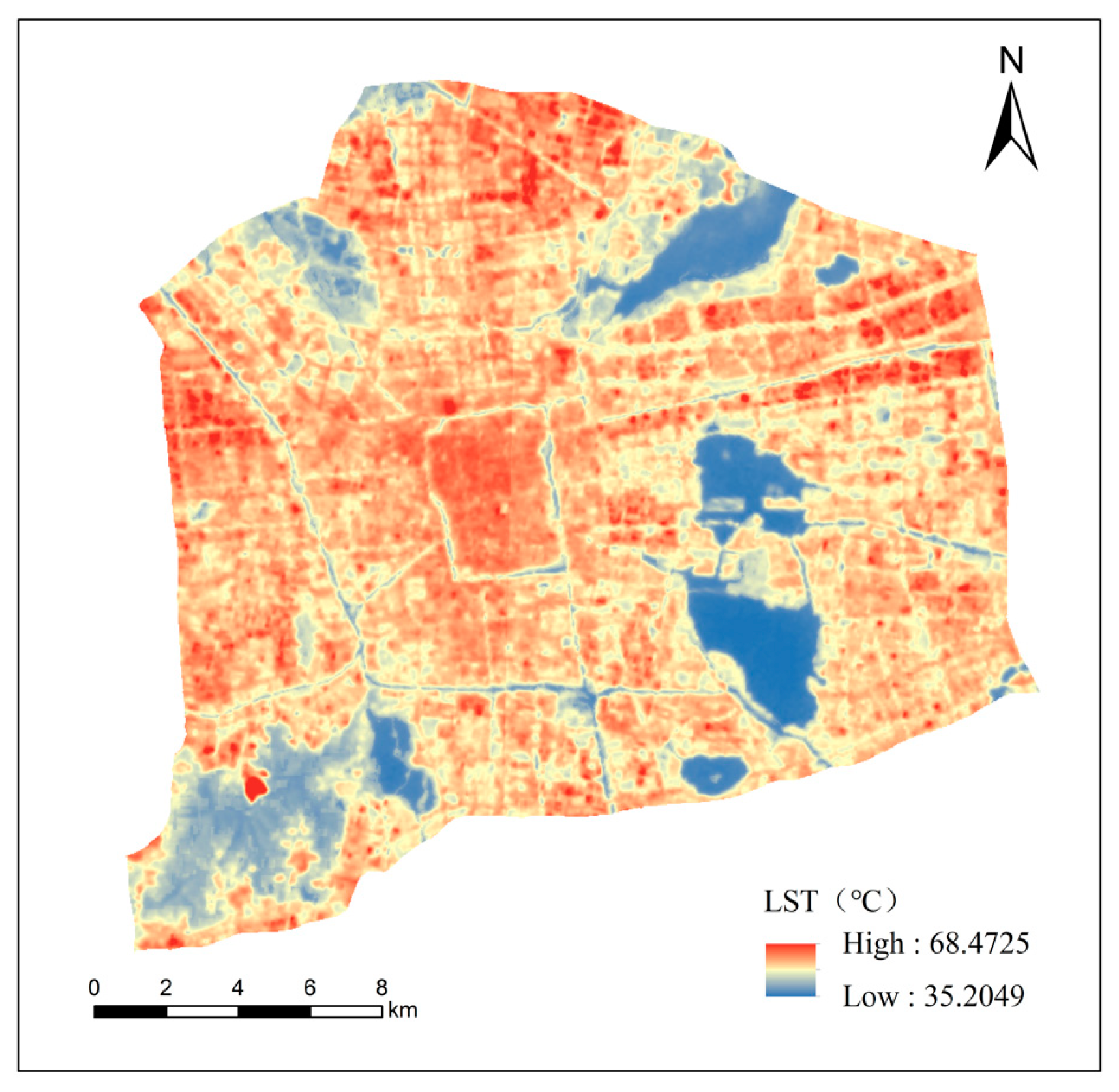
3.1. LST Shows a “High in the Center, Low in the Surroundings” Wedge-Shaped Distribution

The retrieval results (Figure 6) show that within the Middle Ring area of Suzhou, most of the old city area (Gusu District) and parts of Huqiu District and Xiangcheng District, excluding the Wetland Park and Yangcheng Lake, have a high density of buildings, high building density, and high population density, with many human production and living activities, resulting in relatively high LST, with a maximum temperature of 50 °C. In the eastern area (industrial park), there are a large number of dense residential areas, and the LST along Loujiang Avenue and both sides of the highway reaches a maximum of 56 °C. The southern and southeastern areas (parts of Wuzhong District) have relatively higher terrain, large vegetation coverage, fewer buildings, and relatively lower building density, leading to fewer human production and living activities, resulting in relatively low LST, with large areas below 40 °C. Overall, the distribution of LST shows a wedge-shaped pattern of “high in the center, low in the surroundings”.

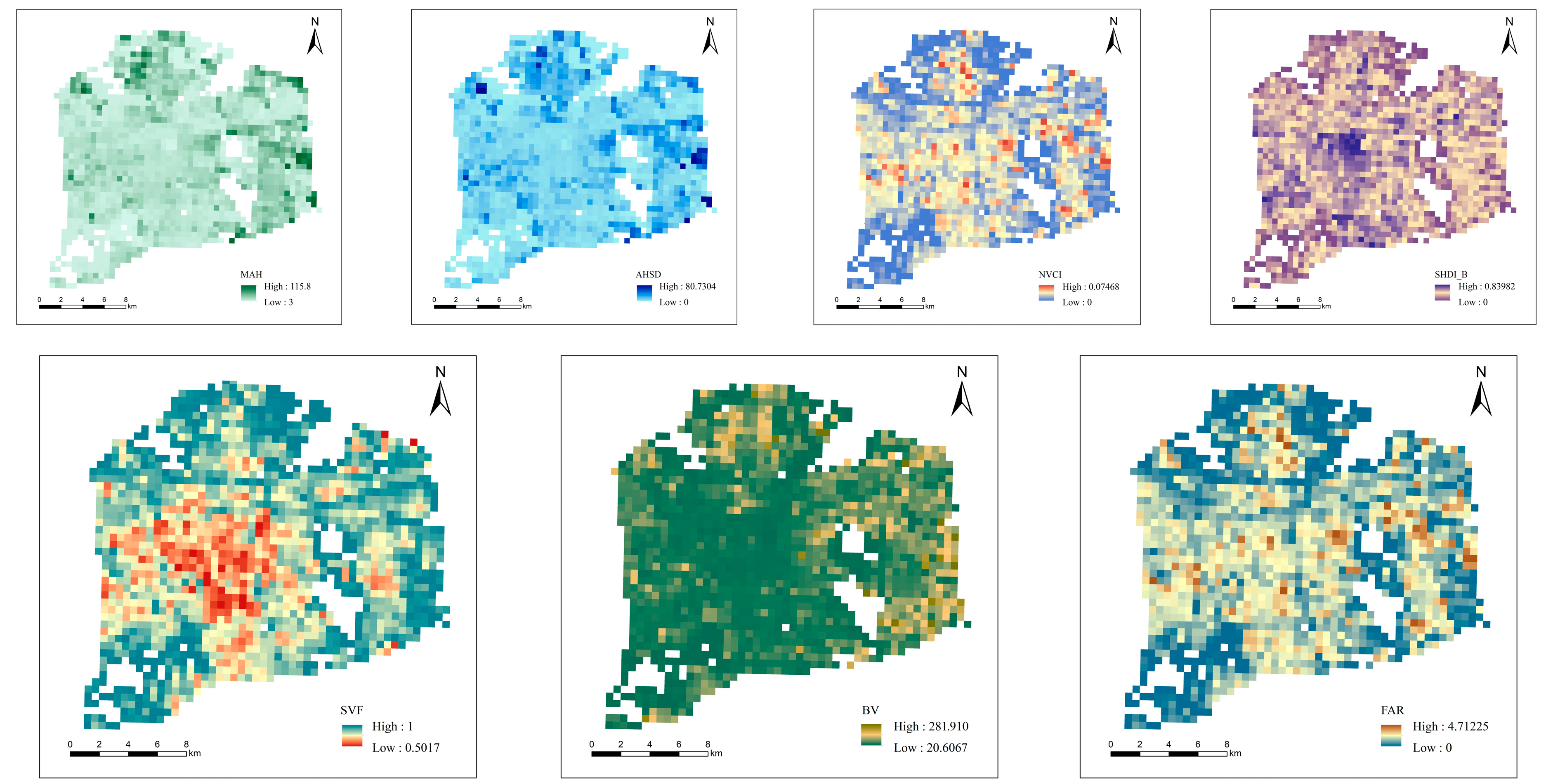
3.2. The Distribution Characteristics of Landscape Metrics Are Generally Obvious

The results of the two-dimensional and three-dimensional landscape pattern metrics calculated using the Fragstats software are shown in Figure 7, Figure 8, Figure 9 and Figure 10. The heat distribution of the building metrics (PLAND_B, LSI_B, ED_B, PD_B, MAH, AHSD, FAR, BV, SHDI_B, SVF, NVCI) more intuitively displays their characteristics.

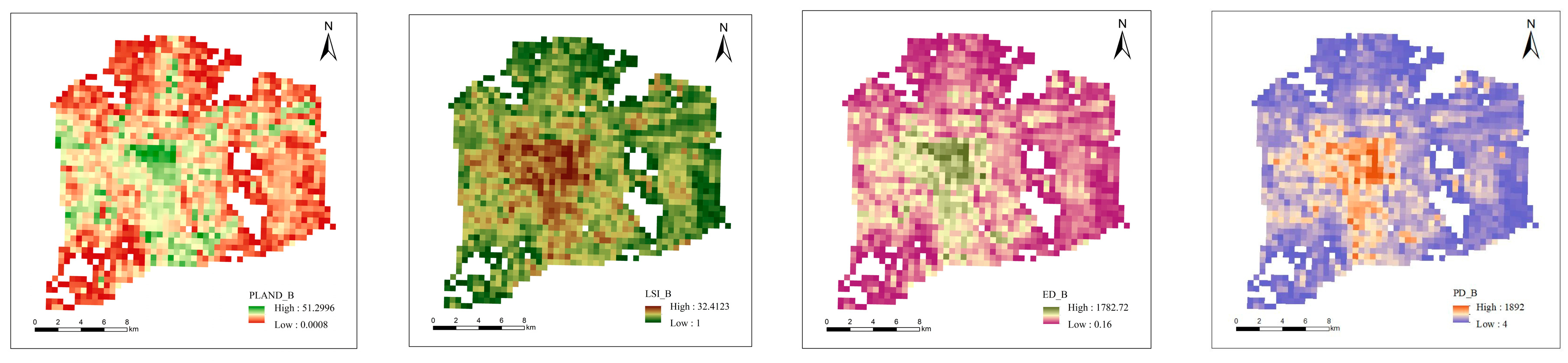
3.2.1. Distribution Characteristics of Building Metrics

(1)

High in the Center, Low in the Surroundings

The heat maps of the building landscape pattern index values show that the four two-dimensional indicators (PLAND_B, LSI_B, ED_B, PD_B) exhibit a “high in the center, low in the surroundings” characteristic (Figure 7). The old city area in the center of Suzhou and some densely populated residential areas have significantly higher coverage rates of PLAND_B, indicating that these areas consist of dense and compact traditional buildings and residential areas. In contrast, in certain high-rise residential areas and CBDs outside the old city, the indicator values are lower, indicating that these areas have sparse building distribution and low building coverage. LSI_B, PD_B, and ED_B also show higher values in the old city area, indicating a high number of patches, a high degree of landscape fragmentation, and high landscape spatial heterogeneity, confirming the dense, compact, and complex characteristics of the old city’s buildings.

In the three-dimensional indicators, SVF, AHSD, and SHDI_B also exhibit a “high in the center, low in the surroundings” characteristic (Figure 8), indicating that the central area of Suzhou has more visible sky area due to buildings and higher variability and richness in building heights.

These indicators are similar to the distribution characteristics of LST, suggesting a possible positive correlation between these indicators and LST.

(2)

Low in the Center, High in the Surroundings

The values of MAH and BV show a “low in the center, high in the surroundings” characteristic (Figure 8). The old city’s numerous traditional buildings and low-rise residential areas result in lower MAH values, and lower BV values indicate smaller or more fragmented building patches per unit area, confirming the higher values of LSI_B and PD_B in the central area. MAH and BV values increase in a wedge-shaped pattern from the center to the surroundings, indicating that high-rise residential areas and CBDs in the periphery lead to higher MAH and BV values.

(3)

No Obvious Characteristics

The calculation of FAR involves the ratio of total building area to land area. The results are scattered and show no obvious characteristics. The distribution of NVCI values is similar to FAR but shows no regular pattern (Figure 8). These results suggest that the relationship between these two indicators and LST might be minimal.

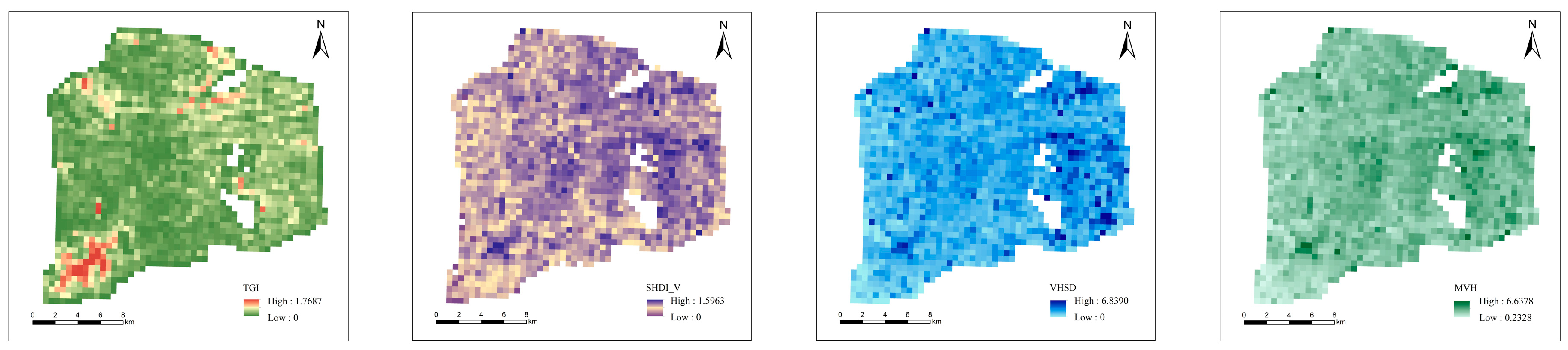
3.2.2. Distribution Characteristics of Vegetation Metrics

(1)

Indicators Also Showing “Low in the Center, High in the Surroundings”

The vegetation coverage rates in different areas also exhibit corresponding features influenced by building coverage characteristics. The results show that the four two-dimensional indicators of vegetation roughly present an opposite pattern to the four two-dimensional building indicators, displaying a “low in the center, high in the surroundings” characteristic (Figure 9). The central area of Suzhou has low PLAND_V, indicating dense building distribution and low vegetation coverage. In areas with less impervious surfaces, vegetation coverage is higher. Modern residential areas with greening requirements have relatively high vegetation coverage, while urban parks and forest-covered areas show the highest vegetation coverage. The values of PD_V, LSI_V, and ED_V also show a wedge-shaped pattern from the center to the surroundings, indicating an increase in the number of vegetation patches, fragmentation, and landscape heterogeneity.

In the three-dimensional vegetation metrics, the distribution of TGI is similar to the two-dimensional PLAND_V.

(2)

No Obvious Characteristics

In the three-dimensional vegetation metrics, the distribution characteristics of MVH, VHSD, and SHDI_V based on height classification show no obvious patterns (Figure 10). The characteristics of these three-dimensional vegetation metrics are mainly based on various factors, such as vegetation species and weather conditions, resulting in no clear distribution pattern within the study area.

3.3. Dominant Impact Indicators on LST under Separate and Combined Building and Vegetation Scenarios

3.3.1. Contribution and Dominant Indicators of Each Metric

(1) The specific contribution rankings of each metric obtained from the BRT model, as shown in Figure 11a, demonstrate the relative importance of each metric when only considering building indicators. The bar chart on the left shows the relative importance of each category variable, expressed as the percentage of explained variance. The results indicate that when only considering the impact of building patterns on LST, three-dimensional building indicators have a slightly higher explanatory power than two-dimensional building indicators. However, the two-dimensional indicator PLAND_B remains the most important indicator positively affecting LST, with an average importance of nearly 27% after 99 iterations of BRT model training. This finding is consistent with Chen et al.’s conclusion that this indicator is dominant in summer. The top five dominant indicators are PLAND_B, SHDI_B, BV, LSI_B, and MAH.

(2) Figure 11b shows the relative importance ranking of vegetation indicators on LST when only considering vegetation indicators. The results indicate that when only considering the impact of vegetation characteristics on LST, the overall explanatory power of two-dimensional vegetation pattern characteristics is higher than that of three-dimensional pattern characteristics. This finding also corroborates Chen et al.‘s research results that horizontal vegetation structure has a higher overall relative impact than vertical vegetation structure [33]. However, TGI is the most significant indicator of all vegetation indicators contributing to LST. The top five dominant indicators are TGI, PD_V, PLAND_V, MVH, and SHDI_V.

(3) When considering the combined impact of all building and vegetation indicators, the overall relative importance ranking of the indicators is shown in Figure 11c. The bar chart displays the explanatory power of the four categories of indicators. The results of variance partitioning indicate that when considering both the two-dimensional and three-dimensional characteristics of vegetation, building pattern indicators still have substantial explanatory power, suggesting that vegetation pattern characteristics have a lesser role in the urban thermal environment compared to building pattern characteristics. The overall importance ranking shows that the top three most important indicators are still building characteristics, with PLAND_B contributing 22.4%, SHDI_B 11.8%, and volume indicator BV 9.9%, following closely. The top five dominant indicators from the BRT model’s relative importance ranking are PLAND_B, SHDI_B, BV, PLAND_V, and PD_V. Overall, LST in Suzhou’s Middle Ring area is significantly influenced by building and vegetation coverage rates, and the diversity of building heights and the volume of buildings and vegetation also significantly impact LST.

The change from Figure 11b to Figure 11c indicates that when only considering the impact of vegetation indicators, the importance ranking is TGI > PD_V > PLAND_V > MVH, while when the impact of building pattern characteristics is included, the importance ranking changes to PLAND_V > PD_V > ED_V > TGI > MVH. The importance of indicators containing vegetation height characteristics, such as TGI and MVH, decreases, suggesting that when considering the impact of buildings, the regulatory effect of vegetation height characteristics on the urban thermal environment diminishes compared to horizontal characteristics.

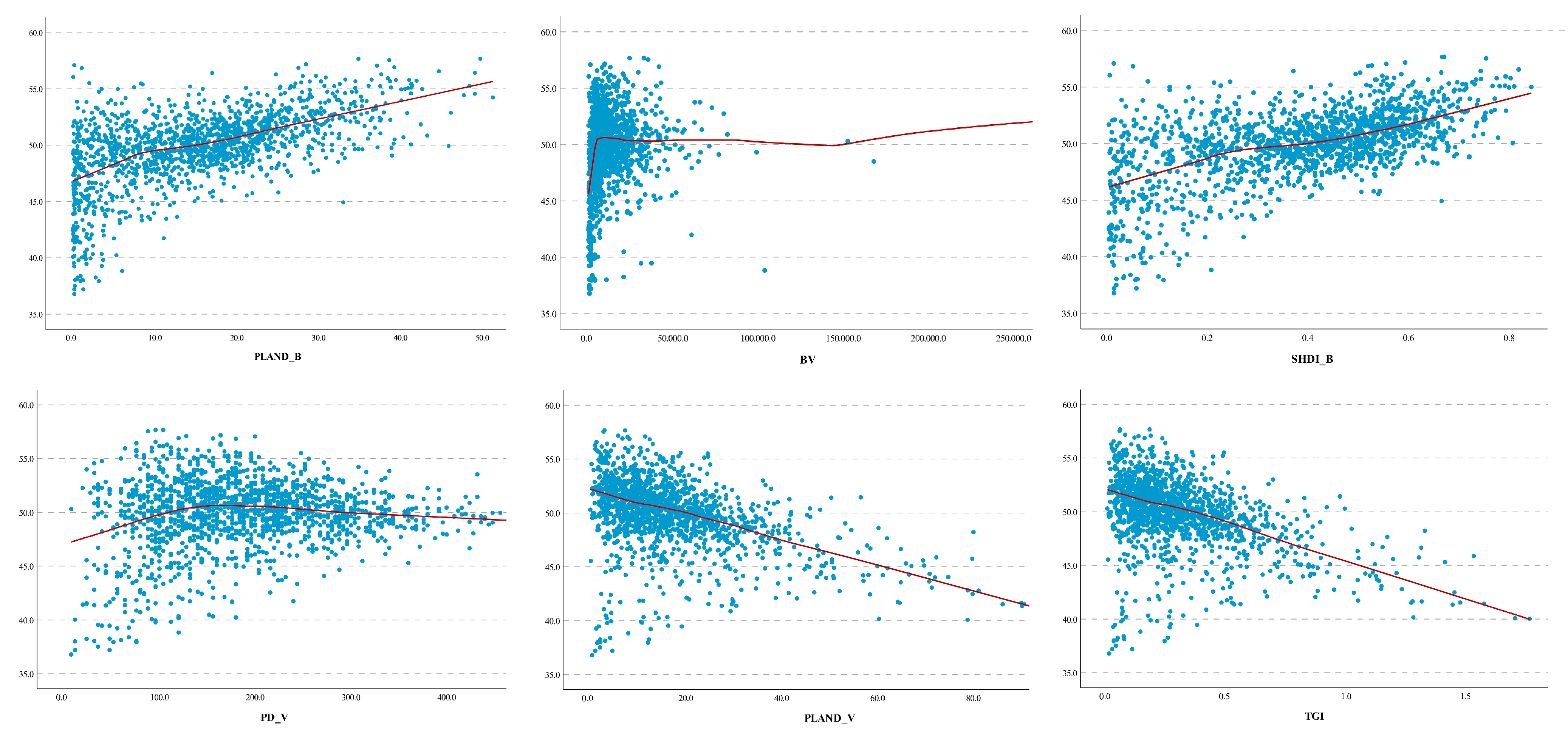
3.3.2. Trends and Correlations

When considering the combined impact of vegetation and buildings on LST, the top six indicators are also the dominant indicators when considering the separate impacts of vegetation and buildings on LST. Therefore, PLAND_B, SHDI_B, BV, PLAND_V, PD_V, and TGI were selected to plot scatter plots with LST and fit curves using the loess (locally weighted regression) non-parametric method, as shown in Figure 12. Correlation analysis was conducted in SPSS 27 to determine the correlations between each indicator and LST (

Table 4. Correlation between dominant indicators and LST.

Landscape Metric	PLAND_B	SHDI_B	BV	PLAND_V	PD_V	TGI
Correlation coefficient	0.573 **	0.570 **	0.116 *	−0.424 **	0.129 **	−0.417 **
Value of ‘p’	<0.001	<0.001	<0.01	<0.001	<0.001	<0.001

* p < 0. 01; ** p < 0. 001.

).

The combined results from the plots and tables show that PLAND_B and SHDI_B are significantly positively correlated with LST, consistent with Zeng et al.’s findings [34]. BV shows a slight decrease followed by an increase and is significantly correlated with LST. Among the vegetation indicators, PLAND_V and TGI are significantly negatively correlated with LST, while PD_V initially shows a warming effect with an increase in PD_V. This indicates that a small increase in the number of vegetation patches with uneven distribution leads to reduced wind speed and poor air circulation, reducing heat dispersion and potentially increasing LST locally. The positive correlation between PD_V and LST is consistent with Wang et al.’s findings [35]. As the density of vegetation patches further increases, the cumulative effect of vegetation coverage begins to manifest, providing more shaded areas and evaporation, leading to a decrease in LST and eventually stabilizing.

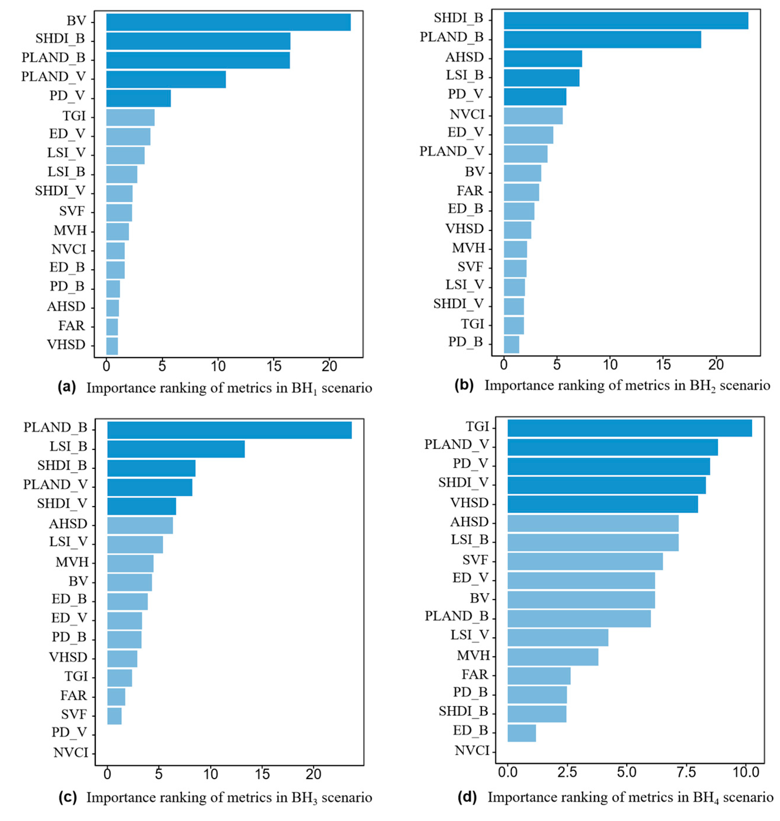
3.4. Differences in Indicator Contribution and Marginal Effects under Different Height Scenarios

The spatial configuration of different building patterns significantly affects the urban thermal environment in both two-dimensional and three-dimensional aspects [36]. The impact of various landscape pattern indicators on LST varies under different height scenarios. To study the specific impact of each indicator on LST under different scenarios, this study selected four sample areas based on different average height (MAH), BH₁, BH₂, BH₃, and BH₄, to explore the changes in the contribution rankings (i.e., dominant indicators) of other landscape indicators on LST under different height scenarios and their marginal effects on LST. Figure 13 shows the contribution rankings of the four sample scenarios derived from the BRT model, and Figure 14 shows the marginal effect values.

3.4.1. Changes in Dominant Indicators

The top five dominant indicators under different heights are as follows: BH₁: BV > SHDI_B > PLAND_B > PLAND_V > PD_V; BH₂: SHDI_B > PLAND_B > AHSD > LSI_B > PD_V; BH₃: PLAND_B > LSI_B > SHDI_B > PLAND_V > SHDI_V; BH₄: TGI > PLAND_V > PD_V > SHDI_V > VHSD.

The results indicate that when building heights are in the BH₁–BH₃ range, PLAND_B and SHDI_B consistently rank among the top five dominant indicators (Figure 13a–c), suggesting that these two building indicators dominate LST changes as building heights increase from BH₁ to BH₃. Therefore, in urban construction, focusing on controlling building coverage rates and the diversity in building heights will help mitigate their impact on the thermal environment. The relative importance ranking of LSI_B increases with building height from BH₁ to BH₃, indicating that the complexity of building patches has a greater impact on LST in higher areas. Other indicators, such as BV and AHSD, are dominant only in BH₁ and BH₂, respectively.

Among vegetation indicators, the two-dimensional indicators PLAND_V and PD_V jointly dominate LST changes in the BH₁ area, along with building indicators, corroborating Wang et al.’s conclusion that the vegetation indicators PLAND_V and PD_V, along with building indicators, are important in influencing LST [35]. Combined with the marginal effect diagram (Figure 14), when building indicators cannot be controlled in the BH₁ area, increasing vegetation coverage rates, reducing patch density per unit area, and controlling landscape fragmentation can reduce LST. The three-dimensional indicator SHDI_V also dominates LST changes in the BH₃ area, suggesting that in areas with building heights of 20–35 m, adopting diverse vegetation group heights can mitigate the thermal environment. In the BH₄ (>35 m) scenario, the top five contributing indicators are all vegetation indicators, indicating that when building heights increase to BH₄, vegetation indicators dominate the impact on LST (Figure 13d). The marginal effects graph shows that increasing three-dimensional greenery, vegetation coverage rates, reducing patch density per unit area, and enriching vegetation group heights can all mitigate LST.

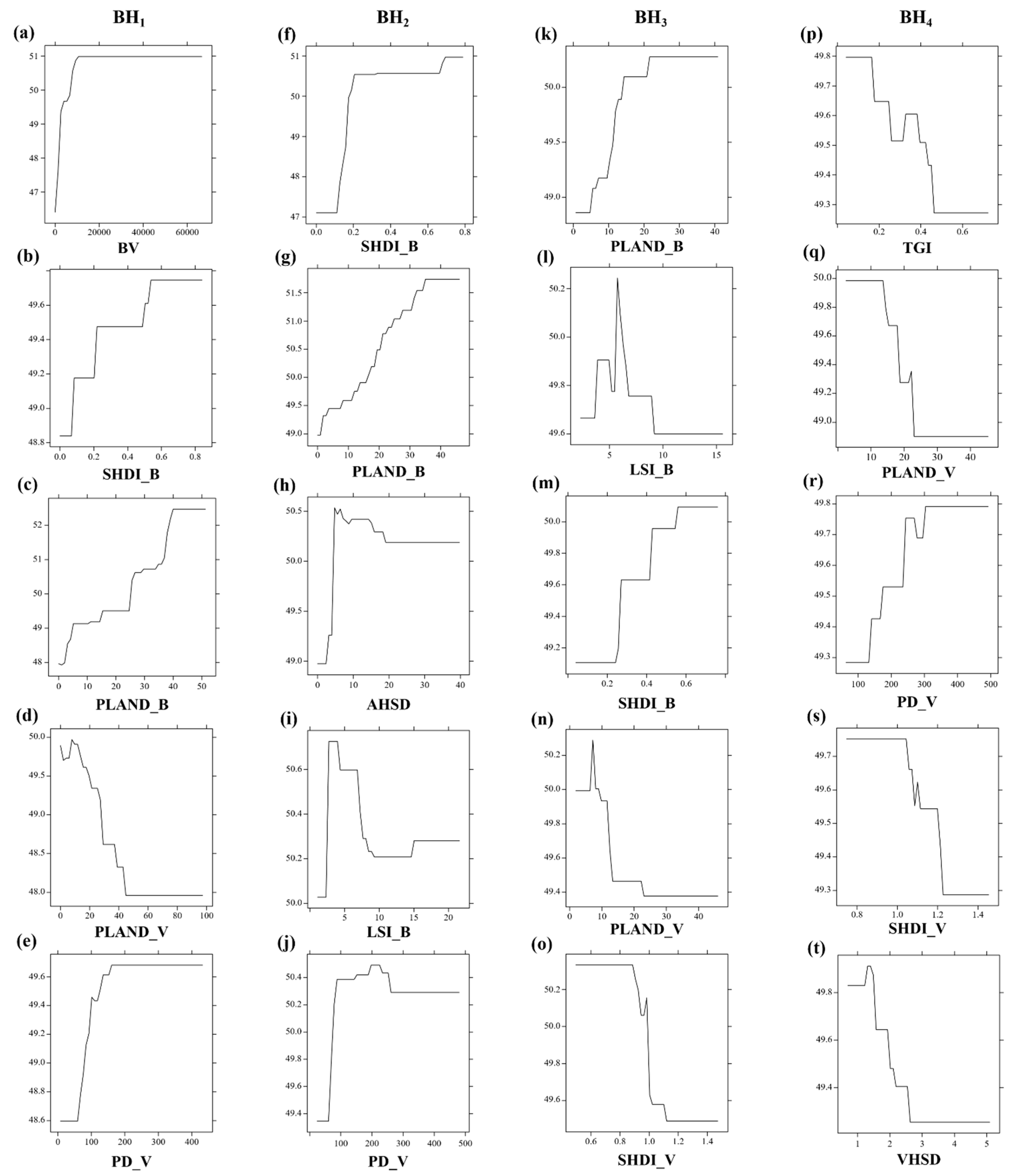
3.4.2. Marginal Effects

Figure 14 shows the marginal effects of the top five contributing indicators under the four scenarios.

The results indicate that in the BH₁, BH₂, and BH₃ scenarios, high PLAND_B and SHDI_B values may lead to high LST, with ∆T reaching 4.5°, 2.7°, and 1.6° (PLAND_B) and 0.9°, 1.2°, and 2° (SHDI_B), respectively. As height increases from BH₁ to BH₃, the warming effect of PLAND_B decreases. In contrast, the warming effect of SHDI_B increases, suggesting that more attention should be paid to controlling the diversity of building heights in this height range. AHSD and PD_V also have a warming effect on LST, but the degree is lower, with smaller ∆T values. High PLAND_V values can effectively reduce LST (∆T up to nearly 1.7°), indicating that increasing PLAND_V in urban construction, especially in areas with heights of 0–10 m and 20–35 m, can effectively alleviate the thermal environment. However, it is worth noting that in the BH₁ scenario, the cooling effect of vegetation coverage rate PLAND_V reaches a threshold when it increases to 45%. In contrast, in the BH₃ scenario, the threshold decreases to 23%, indicating that excessive increase in vegetation coverage rate will not effectively alleviate LST.

In the BH₄ scenario, higher PLAND_V, SHDI_V, VHSD, and TGI values can reduce LST, with ∆T values of 0.65°, 0.57°, 0.65°, and 0.55°, respectively. When planning vegetation, the thresholds of these indicators should be considered as 22%, 2.6 m, 1.2, and 0.48, respectively.

4. Discussion

4.1. How Do Two-Dimensional and Three-Dimensional Urban Building and Vegetation Patterns Specifically Affect LST?

This study explored the relative importance and impact trends of different two-dimensional and three-dimensional landscape metrics on LST, finding that although almost all indicators can explain the impact on LST, their relative importance varies significantly. Comprehensive previous research shows that this is related to the intrinsic performance characteristics of buildings and vegetation and their interactions with the environment.

4.1.1. Specific Impact of Two-Dimensional and Three-Dimensional Urban Building Patterns on LST

When considering only the impact of building morphology, among the 11 building indicators, the two-dimensional indicator PLAND_B is the most important positive impact indicator for LST. This is mainly because, in an urban environment, the increase in building coverage is usually closely related to the rise in building density and the expansion of impervious surfaces [23]. This mainly manifests in the suppression of natural ventilation potential [37,38] and the enhanced ability to absorb solar radiation heat [39]. The importance of the three-dimensional building indicators SHDI_B and BV follows and significantly impacts LST. This may be because higher diversity in building heights leads to less shadow coverage from high-rise buildings in certain areas, exposing more ground to sunlight and increasing direct absorption of solar radiation [37]. Additionally, larger building volumes can absorb and store more solar radiation heat, increasing LST due to their higher heat capacity.

4.1.2. Specific Impact of Two-Dimensional and Three-Dimensional Urban Vegetation Characteristics on LST

The assessment results show that when considering only the impact of vegetation, among all vegetation indicators, TGI contributes the most to the cooling effect on LST. The significant cooling effect of TGI on LST may be because the increase in TGI implies a rise in three-dimensional green volume, which influences air flow and heat exchange, having a crucial impact on temperature [40]. This negative impact on LST is consistent with Zeng et al.’s research findings [34]. PLAND_V is the most important two-dimensional vegetation indicator, where high PLAND_V values help improve the thermal environment. This is due to the more apparent effect of vegetation transpiration as vegetation coverage increases [41]. Moreover, the increase in urban landscape surface roughness promotes air circulation [42], facilitating heat transfer to the atmosphere [43], thereby reducing LST. The two-dimensional indicator PD_V has a certain positive effect on LST. Higher PD_V values mean more vegetation patches with uneven distribution, which can locally increase LST. Fragmented patches reduce wind speed and hinder air circulation, decreasing heat dissipation.

4.1.3. Combined Impact of Two-Dimensional and Three-Dimensional Building and Vegetation Patterns on LST

When considering the combined impact of building and vegetation patterns, the relative contributions of the indicators are ranked as follows: PLAND_B > SHDI_B > building volume BV > PLAND_V > PD_V > TGI. The most important indicators are still building characteristics, and their ranking does not change. However, the ranking of dominant vegetation indicators changes, with the horizontal characteristics of vegetation becoming more important than the vertical characteristics. This may be due to several factors: the interaction between buildings and vegetation might lead to different impact patterns when both are considered.

Specifically, the height and volume characteristics of vegetation directly influence its ability to absorb and scatter solar radiation. Taller vegetation can provide larger shaded areas, effectively reducing ground temperature [19,44]. However, when considering the impact of buildings on LST, building layout, height, and materials can change wind speed and direction, affecting heat diffusion and distribution [45,46]. In this context, horizontal vegetation coverage characteristics like coverage rate and continuity become more important than vegetation height, as they can provide continuous cooling effects in densely built urban environments, creating a better cooling environment.

Additionally, the presence of buildings can limit the expansion of vegetation coverage, making the vegetation coverage rate a crucial factor in influencing the intensity and spatial distribution of the urban heat island effect. Therefore, when considering the combined impact of buildings, the importance of horizontal vegetation characteristics increases.

4.2. How Do Various Indicators Affect LST under Different Building Heights?

4.2.1. Changes in Indicator Importance and Reasons

In urban areas with different building heights, the importance of various indicators on LST changes continuously. The combined bar chart in Figure 15 more intuitively shows the changes in each indicator.

In low- and medium-building-height areas (BH₁, BH₂, BH₃), the relative importance of the two-dimensional building indicators PLAND_B, LSI_B, ED_B, and PD_B increases with building height. This phenomenon indicates that building coverage rate, complexity, and other characteristics that impact ground temperature are influenced by changes in building height. As height increases from BH₁ to BH₃, the importance of three-dimensional building indicators such as BV and SHDI_B decreases, while the importance of various vegetation indicators increases. When building height reaches BH₄, the relative importance of vegetation indicators (TGI, PLAND_V, etc.) surpasses that of building indicators. This may be because, in low- and medium-height-building areas, the high building density means vegetation can cool LST through transpiration and shading. However, the limited amount of vegetation in densely developed areas restricts its cooling impact. In high-rise buildings, the thermal properties of building materials may affect their ability to absorb and release heat [47]. Compared to this, vegetation areas, due to higher moisture content, may have higher heat capacity and transpiration cooling effects. Therefore, in areas with taller buildings, vegetation’s impact on cooling LST is more significant, and urban planting plans should prioritize it in urban construction.

4.2.2. Changes in Marginal Effect Thresholds

From the contribution results, it can be seen that the relative contribution of building coverage PLAND_B to surface temperature is relatively high at all heights and gradually increases with height from BH₁ to BH₃. The turning points of the warming effect of PLAND_B at BH₁, BH₂, and BH₃ are 40.8%, 35%, and 22.5%, respectively, suggesting that as the height increases the warming due to the increase in PLAND_B reaches the threshold value faster. This means that in areas of low-rise buildings, even if the coverage is high, its impact on temperature is relatively small; while in areas of high-rise buildings, a small increase in coverage may lead to a significant increase in surface temperature. Therefore, in the process of urban planning and design, planners should minimize the number of areas with dense high-rise building clusters. Since most vegetation indicators significantly cool LST, this study discusses the changes and applications of the marginal effects of PLAND_V and SHDI_V, which mainly cool LST, in different height areas.

As building height increases from BH₁ to BH₄, the turning point for PLAND_V’s impact on LST decreases from 40% to 22%, and the cooling threshold increases from 48° to 49.4° and then to 48.9°. Overall, as building height increases, the cooling turning point for this indicator occurs earlier, reaches the threshold more quickly, and its cooling effect worsens. Therefore, in urban construction, increasing vegetation coverage will achieve the best cooling effect in areas with low building heights (BH₁). In areas with high building heights, the cooling effect of increasing vegetation coverage is not obvious, requiring the enhancement of other vegetation indicators such as TGI (∆T = 0.55°) and VHSD (∆T = 0.65°) to assist in cooling.

As an advantageous indicator in BH₃ and BH₄, the cooling effect of SHDI_V strengthens as height increases from BH₃ to BH₄, with the turning point rising from 1.1 to 1.2. It reaches the threshold more slowly, and the latter’s cooling magnitude is greater. This suggests that adjusting the diversity of vegetation height SHDI_V in higher areas will have greater benefits.

4.3. Advantages and Limitations

This study combines building height and vegetation height, considering comprehensive three-dimensional landscape indicators and visualizing them, revealing the differences in LST influencing factors in Suzhou’s urban area. However, there are certain limitations. First, this study aims to retrieve and estimate urban canopy data using GF-2 satellite images. Although previous studies, such as the work by Bai et al. [25], have shown that this method can reliably retrieve vegetation height to some extent, it cannot achieve the highest accuracy. In future research, it is planned to introduce LiDAR (light detection and ranging) and SAR (synthetic-aperture radar) technologies for more precise measurement of vegetation height. Secondly, this study utilizes multiple data sources. While this strategy helps in comprehensive analysis, it inevitably introduces certain uncertainties. Specifically, the building height estimated indirectly through floor data may deviate from the actual value, potentially affecting the accurate assessment of building thermal properties [48]. Additionally, the building data used were acquired before 2019, whereas the satellite image data for LST retrieval were collected after this time. Given the possible changes in urban land use and cover types over this period, these changes may impact the accurate retrieval of LST, introducing additional uncertainties. Therefore, future analysis and interpretation of research results will cautiously consider these potential data inconsistencies.

5. Conclusions

This study employed the BRT model to explore the separate and combined relative contributions and marginal effects of two-dimensional and three-dimensional building and vegetation landscape patterns on LST in Suzhou’s Middle Ring area. It also investigated the changes in major landscape indicators affecting LST under four different building height scenarios. The main research findings are as follows:

(1)

When considering only the impact of building patterns on LST, three-dimensional building indicators have slightly higher explanatory power for LST than two-dimensional building indicators. Still, the two-dimensional building indicator PLAND_B remains the most important positive impact indicator for LST. When considering only the impact of vegetation, the overall explanatory power of two-dimensional vegetation indicators is higher than that of three-dimensional indicators. Still, the three-dimensional indicator TGI is the most significant contributor to LST.

(2)

When considering the combined impact of buildings and vegetation, building pattern indicators still have substantial explanatory power, and vegetation pattern characteristics have a lesser role in the urban thermal environment compared to building pattern characteristics. Additionally, building landscape patterns can affect the cooling benefits of vegetation landscape patterns on the urban thermal environment. In contrast, the impact of buildings on the urban thermal environment is less influenced by vegetation. When considering the combined impact of buildings and vegetation, the importance of two-dimensional vegetation indicators in regulating the urban thermal environment increases due to the influence of building patterns, indicating that horizontal vegetation patch coverage plays a more critical role in regulating the urban thermal environment compared to height characteristics.

(3)

Differences in building heights significantly impact the contribution of each indicator. In areas with lower building heights, PLAND_B and SHDI_B consistently rank among the top five dominant indicators. As height increases from BH₁ to BH₃, the warming effect of PLAND_B decreases while the warming effect of SHDI_B increases, highlighting the importance of controlling the diversity of building heights in such height variations. In areas with higher building heights, the vegetation indicators TGI, PLAND_V, PD_V, SHDI_V, and VHSD rank among the top five contributors to LST, with vegetation indicators dominating. As building height increases, the cooling turning point for PLAND_V occurs earlier, the threshold rises, and the cooling effect worsens. Therefore, in BH₁, increasing PLAND_V can achieve a good cooling effect, while in higher areas, enhancing other vegetation indicators can strengthen the cooling effect.

In this study, we used a BRT model that is highly accurate and reliable in predicting the urban heat island effect. Relative to other methods, after screening the indicators that have the greatest impact on surface temperature, it can go further to predict more accurate impact values, i.e., thresholds, such as the conclusions drawn in this study: with the growth of building heights, the inflection point of the effect of vegetation cover PLAND_V on LST decreases from 40% to 22%, so decision-makers will achieve a better cooling effect by increasing vegetation cover in areas with buildings of lower heights, and when this value reaches about 40%, increasing vegetation cover will no longer have a cooling effect. The specific predicted values derived in this paper can be used as reference indicators for planning and designing buildings and green spaces in cities, which will provide accurate data support for urban planning as well as for policymakers and urban planners to avoid exacerbation of thermal environments.

References

1. IPCC-Special-Report. 2024. Available online: https://www.ipcc.ch/site/assets/uploads/sites/2/2019/09/IPCC-Special-Report-1.5-SPM_zh.pdf (accessed on 29 May 2024).
2. Manley, G. On the frequency of snowfall in metropolitan England. Q. J. R. Meteorol. Soc. 1958, 84, 70–72. [Google Scholar] [CrossRef]
3. Kalnay, E.; Cai, M. Corrigendum: Impact of Urbanization and Land-Use Change on Climate. Nature 2003, 423, 528–531. [Google Scholar] [CrossRef] [PubMed]
4. Campbell, S.; Remenyi, T.A.; White, C.J.; Johnston, F.H. Heatwave and Health Impact Research: A Global Review. Health Place 2018, 53, 210–218. [Google Scholar] [CrossRef] [PubMed]
5. Chen, S.; REN, H.; YE, X.; Dong, J.; Zheng, Y. Geometry and adjacency effects in urban land surface temperature retrieval from high-spatial-resolution thermal infrared images. Remote Sens. Environ. 2021, 262, 112518. [Google Scholar] [CrossRef]
6. Kasimu, A.; Zhang, X.; Liang, H. The spatial relationship between seasonal surface temperature and landscape pattern of the urban agglomeration on the northern slope of the Tianshan Mountains. Geogr. Res. 2024, 43, 1267–1287. [Google Scholar]
7. Meng, D.; Li, X.; Gong, H.; Zhao, W. The thermal environment landscape pattern and typical urban landscapes effect linked with thermal environment in Beijing. Acta Ecol. Sin. 2010, 30, 3491–3500. [Google Scholar]
8. Xiang, Y.; Zhou, Z. Influence of blue-green spatial landscape pattern on urban heat island. Chin. Landsc. Archit. 2023, 39, 105–110. [Google Scholar] [CrossRef]
9. Peng, J.; Xie, P.; Liu, Y.; Ma, J. Urban Thermal Environment Dynamics and Associated Landscape Pattern Factors: A Case Study in the Beijing Metropolitan Region. Remote Sens. Environ. 2016, 173, 145–155. [Google Scholar] [CrossRef]
10. Chen, A.; Sun, R.; Chen, L. Applicability of traditional landscape metrics in evaluating urban heat island effect. Chin. J. Appl. Ecol. 2012, 23, 2077–2086. [Google Scholar] [CrossRef]
11. Huang, H.; Yun, Y.; Zhao, R. Key Parameters in Urban Form Layout for WeakeningUrban Heat Island Intensity and Its Response Mechanism. J. Civ. Archit. Environ. Eng. 2014, 36, 95–102. [Google Scholar]
12. Zhou, W.; Huang, G.; Cadenasso, M.L. Does Spatial Configuration Matter? Understanding the Effects of Land Cover Pattern on Land Surface Temperature in Urban Landscapes. Landsc. Urban Plan. 2011, 102, 54–63. [Google Scholar] [CrossRef]
13. Yu, X.; Xu, G.; Liu, Y.; Xiao, Y. Influences of 3D features of buildings on land surface temperature: A case study in the Yangtze River Delta urban agglomeration. China Environ. Sci. 2021, 41, 5806–5816. [Google Scholar] [CrossRef]
14. Guo, F.; Wu, Q.; Schlink, U. 3D Building Configuration as the Driver of Diurnal and Nocturnal Land Surface Temperatures: Application in Beijing’s Old City. Build. Environ. 2021, 206, 108354. [Google Scholar] [CrossRef]
15. Jiang, Y.; Li, Y.; Shi, T.; Han, X. The Simulation of Thermal Environment and Ecological Energy Conservation in Urban Residential Areas. J. Shenyang Jianzhu Univ. 2018, 34, 1145–1152. [Google Scholar]
16. Srivanit, M.; Kazunori, H. The Influence of Urban Morphology Indicators on Summer Diurnal Range of Urban Climate in Bangkok Metropolitan Area. Thailand. Int. J. Civ. Environ. Eng. 2011, 11, 34–46. [Google Scholar]
17. Xu, H.; Li, C.; Hu, Y.; Li, S.; Kong, R.; Zhang, Z. Quantifying the Effects of 2D/3D Urban Landscape Patterns on Land Surface Temperature: A Perspective from Cities of Different Sizes. Build. Environ. 2023, 233, 110085. [Google Scholar] [CrossRef]
18. Luo, P.; Yu, B.; Li, P.; Liang, P.; Zhang, Q.; Yang, L. Understanding the Relationship between 2D/3D Variables and Land Surface Temperature in Plain and Mountainous Cities: Relative Importance and Interaction Effects. Build. Environ. 2023, 245, 110959. [Google Scholar] [CrossRef]
19. Liao, J.; Tan, X.; Li, J. Evaluating the Vertical Cooling Performances of Urban Vegetation Scenarios in a Residential Environment. J. Build. Eng. 2021, 39, 102313. [Google Scholar] [CrossRef]
20. Liu, M.; Ma, J.; Zhou, R.; Li, C.; Li, D.; Hu, Y. High-Resolution Mapping of Mainland China’s Urban Floor Area. Landsc. Urban Plan. 2021, 214, 104187. [Google Scholar] [CrossRef]
21. Alavipanah, S.; Schreyer, J.; Haase, D.; Lakes, T.; Qureshi, S. The Effect of Multi-Dimensional Indicators on Urban Thermal Conditions. J. Clean. Prod. 2018, 177, 115–123. [Google Scholar] [CrossRef]
22. Zhou, W.; Tian, Y. Effects of urban three-dimensional morphology on thermal environment: A review. Acta Ecol. Sin. 2020, 40, 416–427. [Google Scholar]
23. Alexander, C. Influence of the Proportion, Height and Proximity of Vegetation and Buildings on Urban Land Surface Temperature. Int. J. Appl. Earth Obs. Geoinf. 2021, 95, 102265. [Google Scholar] [CrossRef]
24. Hu, X.; Yan, H.; Wang, D.; Zhao, Z.; Zhang, G.; Lin, T.; Ye, H. A Promotional Construction Approach for an Urban Three-Dimensional Compactness Model-Law-of-Gravitation-Based. Sustainability 2020, 12, 6777. [Google Scholar] [CrossRef]
25. Bai, X.; Wang, W.; Lin, Z.; Zhang, Y.; Wang, K. Three—dimensional measuring for green space based on high spatial resolution remote sensing images. Remote Sens. Land Resour. 2019, 31, 53–59. [Google Scholar]
26. Shuai, M.; Xie, Y.; Yang, P. Research on the classification of high-resolution remote sensing images based on eCognition. Wirel. Internet Technol. 2018, 15, 98–99. [Google Scholar]
27. Chang, Y.; Xiao, J.; Li, X.; Middel, A.; Zhang, Y.; Gu, Z.; Wu, Y.; He, S. Exploring Diurnal Thermal Variations in Urban Local Climate Zones with ECOSTRESS Land Surface Temperature Data. Remote Sens. Environ. 2021, 263, 112544. [Google Scholar] [CrossRef]
28. Li, Z.; Hu, D. Exploring the Relationship between the 2D/3D Architectural Morphology and Urban Land Surface Temperature Based on a Boosted Regression Tree: A Case Study of Beijing, China. Sustain. Cities Soc. 2022, 78, 103392. [Google Scholar] [CrossRef]
29. Elith, J.; Leathwick, J.R.; Hastie, T. A Working Guide to Boosted Regression Trees. J. Anim. Ecol. 2008, 77, 802–813. [Google Scholar] [CrossRef] [PubMed]
30. Yu, Q.; Ji, W.; Prihodko, L.; Ross, C.W.; Anchang, J.Y.; Hanan, N.P. Study Becomes Insight: Ecological Learning from Machine Learning. Methods Ecol Evol 2021, 12, 2117–2128. [Google Scholar] [CrossRef]
31. Ren, S.; Wang, T.; Guenet, B.; Liu, D.; Cao, Y.; Ding, J.; Smith, P.; Piao, S. Projected Soil Carbon Loss with Warming in Constrained Earth System Models. Nat Commun 2024, 15, 102. [Google Scholar] [CrossRef]
32. Liu, S.; García-Palacios, P.; Tedersoo, L.; Guirado, E.; Van Der Heijden, M.G.A.; Wagg, C.; Chen, D.; Wang, Q.; Wang, J.; Singh, B.K.; et al. Phylotype Diversity within Soil Fungal Functional Groups Drives Ecosystem Stability. Nat. Ecol. Evol. 2022, 6, 900–909. [Google Scholar] [CrossRef]
33. Chen, J.; Zhan, W.; Du, P.; Li, L.; Li, J.; Liu, Z.; Huang, F.; Lai, J.; Xia, J. Seasonally Disparate Responses of Surface Thermal Environment to 2D/3D Urban Morphology. Build. Environ. 2022, 214, 108928. [Google Scholar] [CrossRef]
34. Zeng, P.; Sun, F.; Liu, Y.; Tian, T.; Wu, J.; Dong, Q.; Peng, S.; Che, Y. The Influence of the Landscape Pattern on the Urban Land Surface Temperature Varies with the Ratio of Land Components: Insights from 2D/3D Building/Vegetation Metrics. Sustain. Cities Soc. 2022, 78, 103599. [Google Scholar] [CrossRef]
35. Wang, Q.; Wang, X.; Meng, Y.; Zhou, Y.; Wang, H. Exploring the Impact of Urban Features on the Spatial Variation of Land Surface Temperature within the Diurnal Cycle. Sustain. Cities Soc. 2023, 91, 104432. [Google Scholar] [CrossRef]
36. Han, S.; Hou, H.; Estoque, R.C.; Zheng, Y.; Shen, C.; Murayama, Y.; Pan, J.; Wang, B.; Hu, T. Seasonal Effects of Urban Morphology on Land Surface Temperature in a Three-Dimensional Perspective: A Case Study in Hangzhou, China. Build. Environ. 2023, 228, 109913. [Google Scholar] [CrossRef]
37. Sun, F.; Liu, M.; Wang, Y.; Wang, H.; Che, Y. The Effects of 3D Architectural Patterns on the Urban Surface Temperature at a Neighborhood Scale: Relative Contributions and Marginal Effects. J. Clean. Prod. 2020, 258, 120706. [Google Scholar] [CrossRef]
38. Huang, Y.; Tu, R.; Tuerxun, W.; Jia, X.; Zhang, X.; Chen, X. A Community Information Model and Wind Environment Parametric Simulation System for Old Urban Area Microclimate Optimization: A Case Study of Dongshi Town, China. Buildings 2024, 14, 832. [Google Scholar] [CrossRef]
39. Chen, Y.; Yang, J.; Yu, W.; Ren, J.; Xiao, X.; Xia, J.C. Relationship between Urban Spatial Form and Seasonal Land Surface Temperature under Different Grid Scales. Sustain. Cities Soc. 2023, 89, 104374. [Google Scholar] [CrossRef]
40. Chen, X.; Zhao, P.; Hu, Y.; Ouyang, L.; Zhu, L.; Ni, G. Canopy Transpiration and Its Cooling Effect of Three Urban Tree Species in a Subtropical City- Guangzhou, China. Urban For. Urban Green. 2019, 43, 126368. [Google Scholar] [CrossRef]
41. Anderson, M.C.; Kustas, W.P.; Norman, J.M.; Diak, G.T.; Hain, C.R.; Gao, F.; Yang, Y.; Knipper, K.R.; Xue, J.; Yang, Y.; et al. A Brief History of the Thermal IR-Based Two-Source Energy Balance (TSEB) Model—Diagnosing Evapotranspiration from Plant to Global Scales. Agric. For. Meteorol. 2024, 350, 109951. [Google Scholar] [CrossRef]
42. Shen, X.; Liu, H.; Yang, X.; Zhou, X.; An, J.; Yan, D. A Data-Mining-Based Novel Approach to Analyze the Impact of the Characteristics of Urban Ventilation Corridors on Cooling Effect. Buildings 2024, 14, 348. [Google Scholar] [CrossRef]
43. Chan, A.T.; Au, W.T.W.; So, E.S.P. Strategic Guidelines for Street Canyon Geometry to Achieve Sustainable Street Air Quality-Part II: Multiple Canopies and Canyons. Atmos. Environ. 2003, 37, 2761–2772. [Google Scholar] [CrossRef]
44. Sodoudi, S.; Zhang, H.; Chi, X.; Müller, F.; Li, H. The Influence of Spatial Configuration of Green Areas on Microclimate and Thermal Comfort. Urban For. Urban Green. 2018, 34, 85–96. [Google Scholar] [CrossRef]
45. Han, G.; Cai, Z.; Xie, Y.; Zeng, W. Correlation between urban construction and urban heat island A case study in Kaizhou District, Chongqing. J. Chongqing Jianzhu Univ. 2016, 38, 138–147. [Google Scholar]
46. Yang, Y.; Zhang, Z.; Yu, X. A Comparative Study of Pedestrian-Level Wind Environment Based on a Standard Urban Building Model. J. Tongji Univ. 2022, 50, 784–792. [Google Scholar]
47. Liu, W.; Gong, A.; Zhou, J.; Zhan, W. Investigation on Relationships between Urban Building Materials and Land Surface Temperature through a Multi-resource Remote Sensing Approach. Remote Sens. Inf. 2011, 46–53, 110. [Google Scholar]
48. Schiano-Phan, R.; Weber, F.; Santamouris, M. The Mitigative Potential of Urban Environments and Their Microclimates. Buildings 2015, 5, 783–801. [Google Scholar] [CrossRef]
Figure 1. Technical route diagram.
Buildings 14 02388 g001
Figure 2. The location of the study area.
Buildings 14 02388 g002
Figure 3. Grid method.
Buildings 14 02388 g003
Figure 4. Vegetation height retrieval results for partial areas.
Buildings 14 02388 g004
Figure 5. Spatial distribution of four building height categories.
Buildings 14 02388 g005
Figure 6. Land surface temperature in the study area.
Buildings 14 02388 g006
Figure 7. Visualization results of 2D building pattern metrics.
Buildings 14 02388 g007
Figure 8. Visualization results of 3D building pattern metrics.
Buildings 14 02388 g008
Figure 9. Visualization results of 2D vegetation pattern metrics.
Buildings 14 02388 g009
Figure 10. Visualization results of 3D vegetation pattern metrics.
Buildings 14 02388 g010
Figure 11. Variance and importance explanations.
Buildings 14 02388 g011
Figure 12. Scatter plots and fitted lines for each indicator.
Buildings 14 02388 g012
Figure 13. Relative importance ranking of indicators under BH1–4 scenarios.
Buildings 14 02388 g013
Figure 14. Marginal effects of the dominant indicators under BH1–4 scenarios.
Buildings 14 02388 g014
Figure 15. Bar chart of changes in importance.
Buildings 14 02388 g015