Temperature Distribution in Asphalt Concrete Layers: Impact of Thickness and Cement-Treated Bases with Different Aggregate Sizes and Crumb Rubber

Abstract

The temperature estimation within asphalt concrete (AC) overlaid on cement-stabilized bases (CSB) is necessary for pavement analysis and design. However, the impact of different CSB gradations and rubberized CSB on AC temperature has not been thoroughly investigated. This study aims to clarify this effect by examining two types of CSB with nominal particle aggregate sizes of 25 mm and 31.5 mm, as well as the substitution of 5%, 10%, and 20% graded aggregates with rubber aggregates (RA) in CSB Dmax 25 using Ansys-based numerical simulations. The modelling also investigated 11 scenarios with different AC thicknesses (h_AC) ranging from 6 to 26 cm. The results indicated that CSB Dmax 31.5 reduced the daily maximum temperature fluctuation at the bottom of the AC (∆T_bottomAC) by approximately 8% compared to CSB Dmax 25. The inclusion of 5% RA in CSB Dmax 25 decreased ∆T_bottomAC by up to 20%. Additionally, the rubberized CSB increased the maximum temperature gradient between the top and bottom of the AC (ΔT_maxAC) by 9.5% with 5% RA and a 6 cm AC thickness; however, this increase was insignificant when h_AC exceeded 12 cm. This study also proposed the use of artificial neural network (ANN) models to predict the AC’s temperature distribution based on depth, the time of day, surface paving temperatures, and h_AC. The proposed ANN model demonstrated high accuracy (R² = 0.996 and MSE = 0.000685),which was confirmed by the numerical simulations, with an acceptable RMSE ranging from 0.28 °C to 0.67 °C.

1. Introduction

The semi-rigid pavement structure, consisting of asphalt concrete (AC) surface layers placed on a cement-stabilized base (CSB), is well-suited for arterials, highways, roads with heavy traffic, and high vehicle volumes, as well as for taxiways and aprons in airport pavements, particularly under aggressive thermal conditions [1,2,3,4,5]. However, this pavement is susceptible to reflective cracking that originates from the cracked CSB and propagates to the AC surface [6]. To mitigate this situation, one approach is to incorporate rubber aggregates (RA), ground from end-of-life tires [7], as partial replacements for crushed stone aggregates to form rubberized CSB aggregates [8,9,10]. To explain the better performance of rubberized CSB in preventing thermal shrinkage, Pham et al. [9] investigated the temperature distribution within semi-rigid pavement using an Ansys simulation; the authors reported that the RA addition in CSB helped to reduce thermal absorption and temperature fluctuations in the pavement. In their research, the AC layer thickness was fixed at 13 cm; different amounts of RA were incorporated into the CSB as partial volume replacements for graded aggregates at 0%, 5%, 10%, and 20%. It should also be noted that the utilization of by-products in road construction is widely recognized as a practical solution [11,12,13] that helps to reduce environmental hazards and promote the circular economy for sustainable transportation system development. Typically, rubberized concrete is more impactful than conventional concrete in dispersing traffic loads over a large area of the concrete slab/subbase course interface; the use of rubberized concrete reduces stresses to the subbase compared to the use of a plain concrete slab [14].

The temperature distribution within pavements is influenced by climatic conditions [15], surface characteristics of wearing course [16], traffic loads [17], road materials and structures [9,18], the hydro-thermal regime in roadbeds [19], and the thermal properties of paving materials [20,21,22,23]. In semi-rigid pavements, the bituminous surface layer, AC, exhibits high sensitivity to temperature variations. Its modulus of elasticity is contingent upon the actual operation temperature, which impacts pavement integrity and leads to various stresses such as low-temperature cracking and rutting at high temperatures [24]. The temperature distribution information within AC is necessary when selecting paving material properties for pavement designs that improve pavement performance during specific operational conditions. Some studies recommend that AC thickness should be properly designed by considering the local climatic conditions to mitigate reflective cracking in AC overlaid on CSB. The TCCS 38:2022 standard [25] requires that the total AC thickness is equal to, or greater than, the CSB thickness [25]. However, specific recommendations regarding the optimization of AC thickness for different climatic regions are not specified. Therefore, studies on temperature distribution within AC in semi-rigid pavements using CSB with varying AC thicknesses is necessary to evaluate the related thermal stresses in the pavement structure. Several investigations confirmed that the thermal properties of paving materials significantly influence thermal absorption within road pavements [9,26]. Tran et al. [18] pointed out that the AC thickness significantly impacted the temperature distribution in traditional CSB. The authors also demonstrated the combined effects of CSB properties and AC layer thickness on temperature absorption within the CSB layer [26]. However, no studies have been conducted to investigate the impact of paving thermal properties and AC thickness on the temperature distribution within AC.

Typically, empirical and numerical methods are applied to predict temperature distribution in pavement structures [27,28,29,30,31,32,33]. Based on finite element methods, the latter exhibit the most advantages for various paving materials and structures with varied pavement layer thicknesses [34]. Compared to statistical approaches, numerical simulations only require testing of the thermal properties of each paving material in pavements [18,26,35,36]. The Ansys-based temperature distribution prediction model developed by Thao et al. [10] was validated with field monitoring data, demonstrating a slight RMSE that ranged from 0.35 °C to 0.54 °C. From the valid numerical model, the authors employed temperature distribution prediction for semi-rigid pavement structures using rubberized CSB [9] or varying AC thicknesses [26], etc. Artificial neural network (ANN) methods were also demonstrated as suitable approaches for predicting temperature in road pavements [30,31,37]. In particular, Tran et al. [26] utilized numerical simulation results to propose an ANN model for predicting temperature changes in CSB pavements with varying thicknesses of AC in semi-rigid pavement structures. The authors confirmed highly compatible results in temperature estimation between the numerical and ANN approaches [26].

As briefly summarized above, the numerical simulation model was developed to accurately predict temperature distribution within semi-rigid pavements. Our previous study [18] developed suitable Ansys-based numerical models for temperature prediction in CSB using graded aggregates with nominal maximum aggregate sizes of 31.5 mm (Dmax 31.5), and subsequently confirmed the significant effect of AC thickness on the temperature of control CSB (without the addition of RA). In addition, when CSB Dmax 31.5 was used, an increase in AC thickness resulted in a more significant temperature difference between the top and bottom AC [18]. For our other previous investigations, the temperature distribution within rubberized CSB was also predicted considering different thicknesses of AC overlaid on the base [26]. However, the impact of different CSB gradations and rubberized CSB on the temperature distribution in variable-thickness AC has not been addressed yet. Therefore, this study focuses on the research gap; Dmax 31.5 and Dmax 25 treated with 4% cement were investigated. RA with sizes ranging from 3–6 mm were also considered for replacing 0%, 5%, 10%, and 20% of the volume of graded aggregates ranging from 0.425 mm to 9.5 mm in Dmax 25. All scenarios are assessed across the following 11 distinct thicknesses of AC: 6 cm, 8 cm, 10 cm, 12 cm, 14 cm, 16 cm, 18 cm, 20 cm, 22 cm, 24 cm, and 26 cm. Subsequently, the study developed an ANN model with a dataset obtained through numerical simulations for temperature distribution within the AC according to AC thickness and depth, the time of day, and pavement surface temperature.

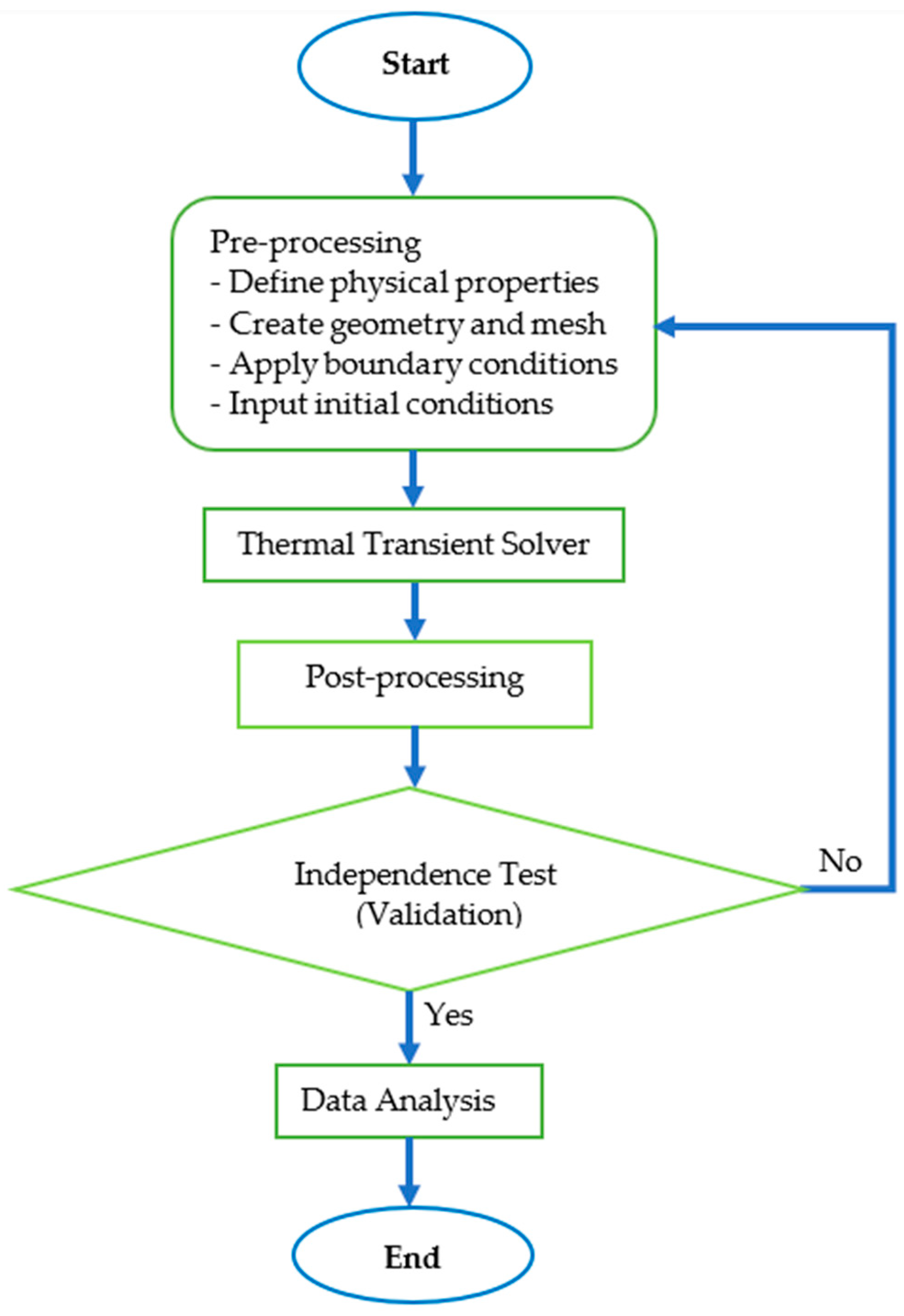
2. Data Collection from Numerical Simulations

This study explores data collection by changing some of the parameters in our previously developed numerical simulations using Ansys 2023 R2 [9,10,18,26]. Note that the software enables the performance of various simulations and analyses across multiple engineering disciplines, including structural analysis, thermal analysis, fluid dynamics, and electromagnetics [38]. The models were validated through rigorous comparison with actual temperature monitoring data in two cases of semi-rigid pavement structures. For the first case, consisting of a 16 cm AC, a 15 cm CSB Dmax 31.5, and a 15 cm subbase Dmax 37.5, the RMSEs between the numerical results and actual monitoring data were insignificant, ranging from 0.35 °C to 0.54 °C) [10]. When a 13 cm AC was placed on a similar base and subbase, the RMSE was small, at around 0.34 °C ÷ 0.48 °C [18]. The results demonstrated higher accuracy than those obtained in previous studies; for example, the RMSE changed from 2.1 °C to 4 °C in a study by Minhoto et al. [39] and an error of up to 3 °C was reported by Zhang et al. [40].

Figure 1 shows the simulation steps of thermal distribution in road pavements using Ansys 2023 R2. It should be recalled that the numerical simulations were based on the one-dimensional heat transfer theory. The boundary conditions and other input parameters of the valid models include, as follows:

• The pavement surface temperature (Tsuf) was obtained from actual field measurements every 10 min from the field monitoring from 28 June to 2 July 2021, as reported by Tran et al. [18];
• One-way heat transfer in the vertical direction was applied. Thus, the surrounding boundary was insulated;
• A 2 m depth was considered adiabatic due to the roadbed temperature being relatively stable during a monitoring period [39];
• The element was meshed to a thickness of 1 cm [41] using 20-node brick elements (SOLID279). TARGE170 and CONTA174 elements were also employed to model the contact behavior between the paving layers [9];
• Thermal parameters of paving materials were related to pavement surface temperature, as obtained from previous studies and presented in

  Table 1. Thermal properties of CSB Dmax 25 with different RA contents [9].

  Thermal Properties		Temperature of CSB (°C)
  		40	45	50	55	60
  CSB 0R	Thermal conductivity, λ (W·(m·°C)−1)	0.899	1.023	1.146	1.270	1.393
  	Specific heat capacity, C (J·(kg·°C)−1)	1280.70	1330.59	1372.54	1408.31	1439.16
  	Density, ρ (kg·m−3)	2265
  CSB 5R	Thermal conductivity, λ (W·(m·°C)−1)	1.442	1.342	1.242	1.142	1.042
  	Specific heat capacity, C (J·(kg·°C)−1)	2032.26	1726.46	1469.70	1251.07	1062.65
  	Density, ρ (kg·m−3)	2294
  CSB 10R	Thermal conductivity, λ (W·(m·°C)−1)	1.113	1.049	0.985	0.921	0.857
  	Specific heat capacity, C (J.(kg.°C)−1)	1780.24	1493.33	1263.27	1074.68	917.28
  	Density, ρ (kg·m−3)	2184
  CSB 20R	Thermal conductivity, λ (W·(m·°C)−1)	1.003	0.930	0.856	0.783	0.709
  	Specific heat capacity, C (J·(kg·°C)−1)	1748.54	1424.53	1170.41	965.78	797.46
  	Density, ρ (kg·m−3)	2174

  and

  Table 2. Thermal properties of AC and CSB Dmax 31.5.

  Paving Materials	Density, ρ (kg·m−3)	Temperature of Materials (°C)	Thermal Conductivity, λ (W·(m·°C)−1)	Specific Heat Capacity, C (J·(kg·°C)−1)
  AC [10]	2387	30	1.59	1068.6
  	2387	35	1.65	1087.8
  	2387	40	1.71	1106.2
  	2387	45	1.77	1124.0
  	2387	50	1.83	1141.1
  	2387	55	1.89	1157.6
  	2387	60	1.95	1173.5
  	2387	65	2.01	1188.9
  	2387	70	2.07	1203.7
  CSB Dmax 31.5 [10]	2371	30	1.44	1063.4
  	2371	35	1.48	1063.9
  	2371	40	1.53	1064.4
  	2371	45	1.58	1064.9
  	2371	50	1.62	1065.3
  	2371	55	1.67	1065.7
  	2371	60	1.72	1066.1
  Aggregate subbase [42]	2187		1.8	964
  Soil subgrade [42]	1418		1.1	840

  [9,10].

In this study, the simulations were applied to analyze the temperature distribution in AC of semi-rigid pavement structures, including, as follows: (i) AC with thickness variations from 6 cm to 26 cm; (ii) a 15 cm CSB; (iii) a 15 cm Dmax 37.5 subbase; and (iv) soil subgrade. It should be noted that different particle gradations of graded aggregates, Dmax 25 and Dmax 31.5, were used for CSB. Additionally, RAs with sizes ranging from 3–6 mm were used to substitute 0%, 5%, 10%, and 20% of the volume of aggregates ranging from 0.425 mm to 9.5 mm in the case of CSB Dmax 25 for further investigation on the effect of RA on temperature distribution within AC. The replacements were assigned 0R, 5R, 10R, and 20R, respectively. Furthermore, the surface pavement temperatures, denoted as T_suf, assigned to the simulation as a boundary condition, were obtained from field monitoring conducted from 28 June to 2 July 2021, as reported by Tran et al. [18]. Note that long-term temperature data collection can be applied to the simulations. The thermal properties of AC, CSB Dmax 25, CSB Dmax 31.5, and rubberized CSB Dmax 25 were investigated in previous studies [9,10] and are presented in Table 1 and Table 2. For the graded aggregates subbase Dmax 37.5 and soil subgrade, the thermal properties were obtained from research conducted by Mammeri et al. [42], and are illustrated in Table 2.

Results from numerical simulations for various cases, including the use of distinct graded aggregates (Dmax 25 and Dmax 31.5) or the incorporation of RA in CSB Dmax 25, are utilized to calculate the maximum temperature difference between the top and bottom of the AC during the day (ΔT_maxAC) and the temperature gradient at the bottom of AC (∆T_bottomAC). Simultaneously, the simulation data from cases of variable-thickness AC layers placed on CSB Dmax 31.5 are obtained to develop an ANN model for predicting temperatures within AC.

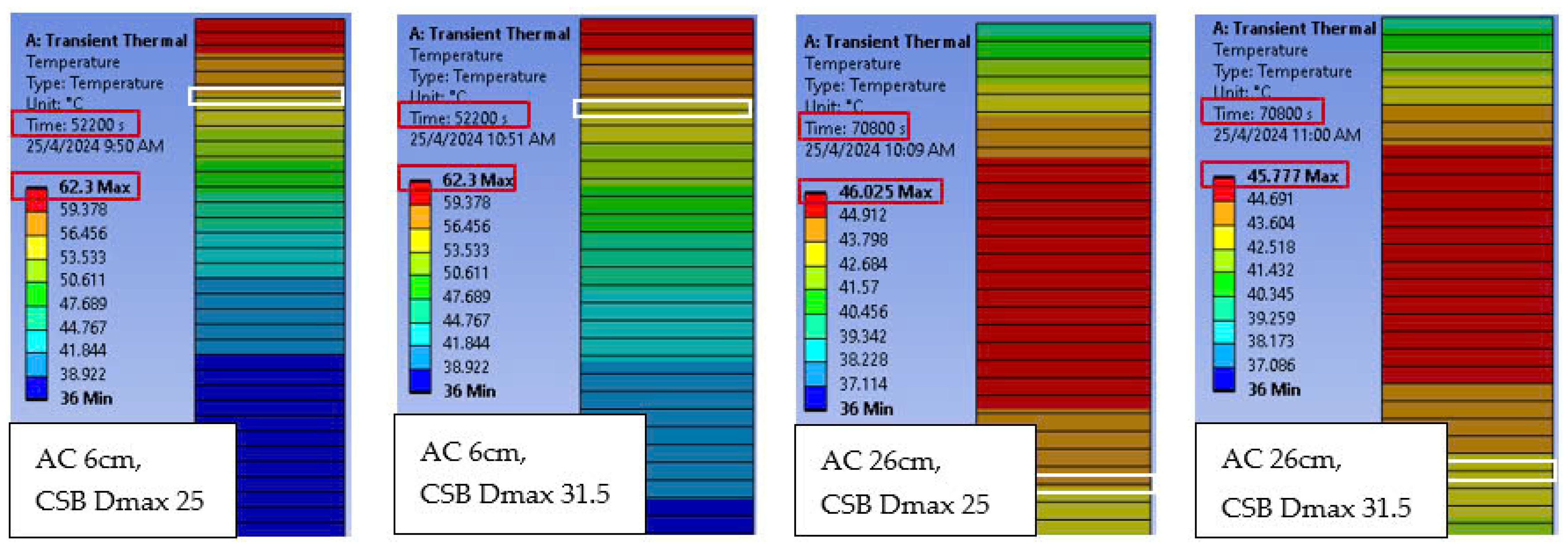
3. Effect of CSB on Temperature Distribution in Variable-Thickness AC Layer

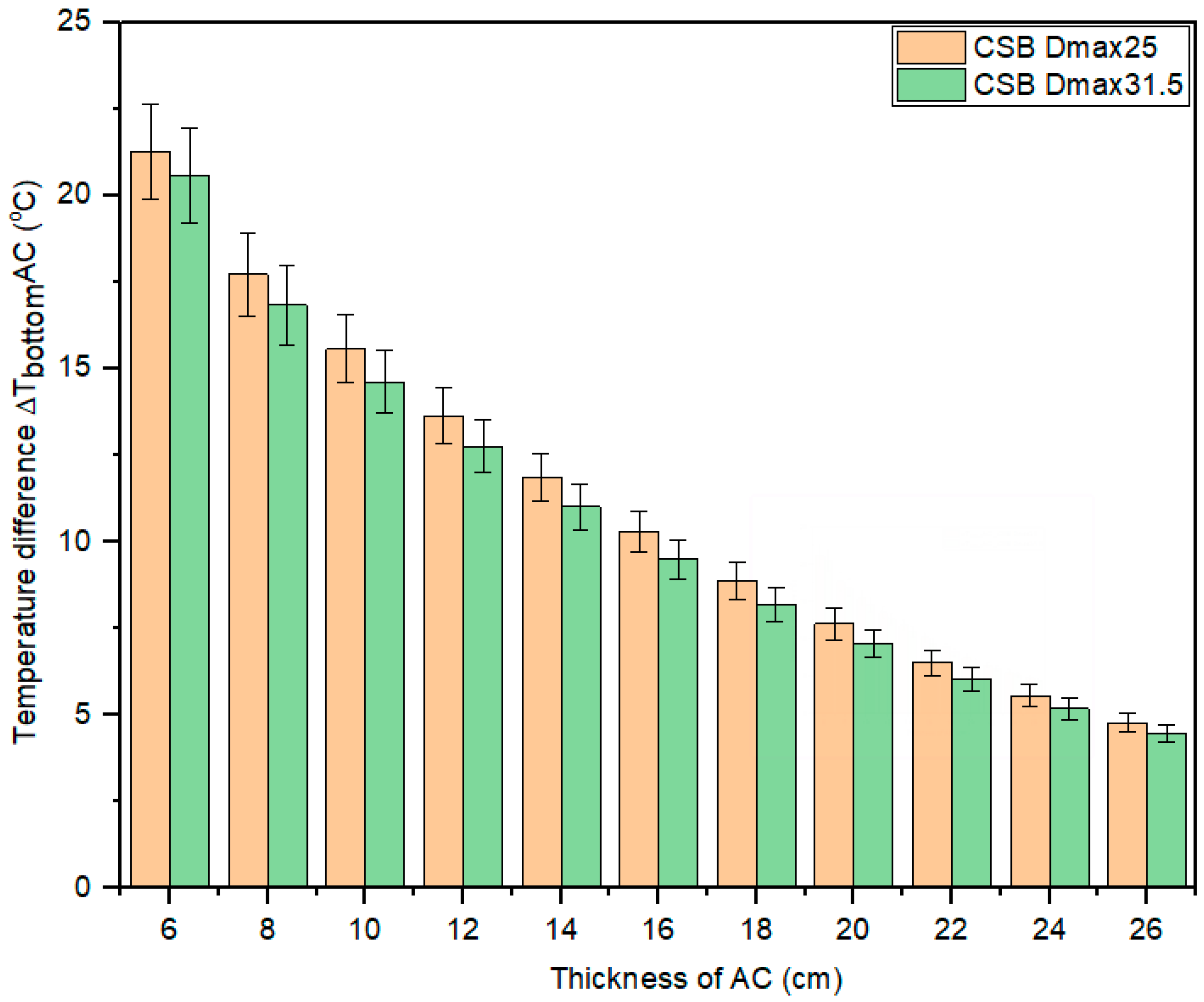
3.1. Effect of Graded Aggregates Gradation of CSB

Figure 2 presents the temperature contours within the AC derived from the Ansys simulation when the bottom of the AC reaches its peak temperature. The findings show that CSB Dmax 31.5 leads to a reduced temperature gradient across the depth of the AC. This phenomenon can be attributed to the base’s higher density and greater compactness, which facilitate faster heat transfer. Consequently, heat within the AC dissipates more rapidly into the base, thus lowering the overall AC temperature. This observation is consistent with previous research findings [22,23]. However, the CSB Dmax 25, characterized by a lower density and reduced compactness, retards the heat conduction process towards the base. Hence, the heat dissipation within the AC is slower, resulting in a higher AC temperature. Furthermore, Figure 2 illustrates that, as the AC thickness increases up to 26 cm (h_AC = 26 cm), the influence of CSB on the temperature distribution within the AC becomes more pronounced compared to scenarios with thinner ACs (h_AC = 6 cm), primarily when CSB Dmax 31.5 is employed. Note that white frame in Figure 2 presents depths of 6 cm and 26 cm, while the red ones indicate the maximum temperature in AC and time at the highest temperature. This observation emphasizes the significance of AC thickness in determining its temperature distribution. Thus, this parameter should be considered in the temperature prediction model developed in Section 4.

From the numerical simulation results of temperature distribution in the AC placed on different CSB using distinct, normal, graded aggregate sizes (Dmax 25 and Dmax 31.5), ∆T_bottomAC and ∆T_maxAC were calculated and presented in Figure 3 and Figure 4, respectively. As can be seen from the figures, a thicker AC layer results in lower temperature fluctuations at the bottom of the AC (∆T_bottomAC) and a higher temperature gradient between the top and bottom of the AC (∆T_maxAC). In addition, CSB Dmax 31.5 causes lower ∆T_bottomAC and higher ∆T_maxAC than CSB Dmax 25 for all cases of AC thicknesses. However, the temperature difference is insignificant when the AC layer becomes thicker.

Table 3. Comparison of CSB Dmax 25 to CSB Dmax 31.5 on temperature fluctuation (∆T_bottomAC and of ∆T_maxAC) (%).

AC thickness (cm)	6	8	10	12	14	16	18	20	22	24	26
ΔTbottomAC change (%)	3.3	5.2	6.5	6.9	7.9	8.3	8.5	8.1	7.9	7.4	7.3
ΔTmaxAC change (%)	−5.5	−4.1	−3.8	−1.9	−1.9	−1.4	−1.0	−0.5	−0.9	−0.6	−0.2

compares the effect of CSB Dmax 25 on these temperature changes (∆T_bottomAC and ∆T_maxAC) with that of CSB Dmax 31.5. CSB Dmax 25 results in a higher average temperature fluctuation at the bottom of the AC (∆T_bottomAC Dmax 25) compared to CSB Dmax 31.5 across all AC thicknesses, with reductions ranging from 3.3% to 8.5%. However, the maximum temperature gradient between the AC top and bottom (∆T_maxAC) of CSB Dmax 31.5 is slightly higher than that of CSB Dmax 25. Note that the difference is insignificant, at only less than 5.5%, and that a thicker AC results in a lower ∆T_maxAC. This observation can be attributed to the dependence of heat transfer in paving materials on thermal properties and the pavement surface temperature during its operation [10,23,26]. Therefore, the temperature transferred to the bottom of the AC decreased as the AC thickness increased. At this stage, the thermal characteristics of AC are primarily affected by paving material properties, and the impact of the surface temperature on the heat transfer of paving materials appears to be negligible.

3.2. Effect of RA Contents in Rubberized CSB on Temperature Distribution in AC

Figure 5 illustrates the AC temperature contours in two thicknesses (6 cm and 26 cm) as the AC bottom temperature peaked and the RA was substituted as part of the graded aggregates in the CSB Dmax 25. Incorporating 5% RA in the CSB resulted in a minimal temperature gradient between the AC top and bottom, and in the lowest maximum temperature at the AC bottom. This occurrence can be explained by the higher density of the rubberized CSB 5R. The property helps to improve its compactness and facilitate a more rapid heat transfer process into the CSB 5R, resulting in a lower heat in the AC. The heat transfer affected by such a material property was confirmed by Chen et al. [22,23]. However, regarding the case of 20R having a lower density and reduced compactness, the CSB is detrimental to the heat conduction process and heat dissipation into the base layer. Therefore, thermal retention within the AC is increased, causing higher temperatures at the bottom. Meanwhile, for CSB 10R, the temperature distribution within the AC appears to be similar to that of the case without the incorporation of RA into the CSB (0R).

Moreover, Figure 2 and Figure 5 also reveal variations in the timing of peak temperatures at different depths throughout the day. Deeper depths exhibit delayed attainment of maximum temperatures (e.g., the maximum temperature at the bottom of a 6 cm AC occurs at 14:30, whereas, for a 26 cm AC layer, it transpires at 19:40). This disparity could be explained by the absorption of thermal energy from solar radiation on the pavement surface that progressively penetrates into the pavement structures. Consequently, a heating time is required for thermal conduction and thermal retention within the paving material. The phenomenon results in a delay in reaching the maximum temperature at different positions far from the pavement surface and in a reduction in the temperature magnitude at deeper depths. Hence, the depth of the material layer and the time of day significantly influence the temperature distribution within the AC.

With regard to the incorporation of different RA into the CSB Dmax 25, ∆T_bottomAC and ∆T_maxAC were obtained and are illustrated in Figure 6 and Figure 7, respectively. Regardless of the incorporation of RA in CSB, the increasing AC thickness reduced the temperature gradient at the AC bottom (∆TbottomAC) and increased temperature fluctuation in AC (∆T_maxAC). Specifically, the ∆T_bottomAC was lowest when CSB 5R Dmax 25 was used for all 11 scenarios of different AC thicknesses. However, the use of CSB 5R Dmax 25 also caused slightly higher ∆T_maxAC, as the AC thickness was less than 12 cm. For thicker AC layers, the gradient was negligible.

To compare the effect of using RA on T_bottomAC and ∆T_maxAC with the reference CSB (0R), the differences in these parameters, in percentages, were calculated and are presented in

Table 4. Comparison of CSB Dmax 25 using RA to the reference CSB 0R on temperature fluctuation (∆T_bottomAC and of ∆T_maxAC) (%).

AC Thickness (cm)		6	8	10	12	14	16	18	20	22	24	26
ΔTbottomAC change (%)	5R	−7.0	−11.6	−14.2	−16.4	−18.0	−19.1	−19.9	−20.4	−20.0	−20.2	−20.4
	10R	−0.5	−1.8	−3.1	−4.2	−5.2	−6.1	−6.7	−7.2	−6.9	−7.2	−7.5
	20R	1.9	1.5	0.6	−0.3	−1.3	−2.1	−2.8	−3.3	−3.1	−3.5	−3.8
ΔTmaxAC change (%)	5R	9.5	7.8	5.4	3.2	1.6	0.8	0.3	0.2	0.0	−0.2	−0.3
	10R	2.4	3.0	2.4	1.6	0.9	0.4	0.2	0.1	0.0	−0.1	−0.2
	20R	−0.4	1.0	1.3	1.1	0.7	0.3	0.2	0.0	0.0	−0.1	−0.2

. It can be seen that an amount of less than 10% of RA reduces temperature fluctuations at the bottom of the AC (∆T_bottomAC). The rubberized CSB 5R exhibits a 7% to 20.4% reduction in ∆T_bottomAC depending on the AC thickness; increasing the bituminous surface thickness resulted in more significant temperature changes. Moreover, Table 4 also demonstrates a slight increase in the temperature distribution within the AC when RAs are used. However, as the thickness of AC exceeds 12 cm, the maximum temperature fluctuation within AC (∆T_maxAC) increases, at around less than 3.2%. The slight increase in the temperature of the AC observed when substituting 5% of RA in CSB is attributed to the RA’s high density and solid nature, and to its detrimental heat dissipation at the bottom of the AC, resulting in a marginal rise in AC temperature.

4. Model Development ANN for Temperature Distribution Prediction in AC

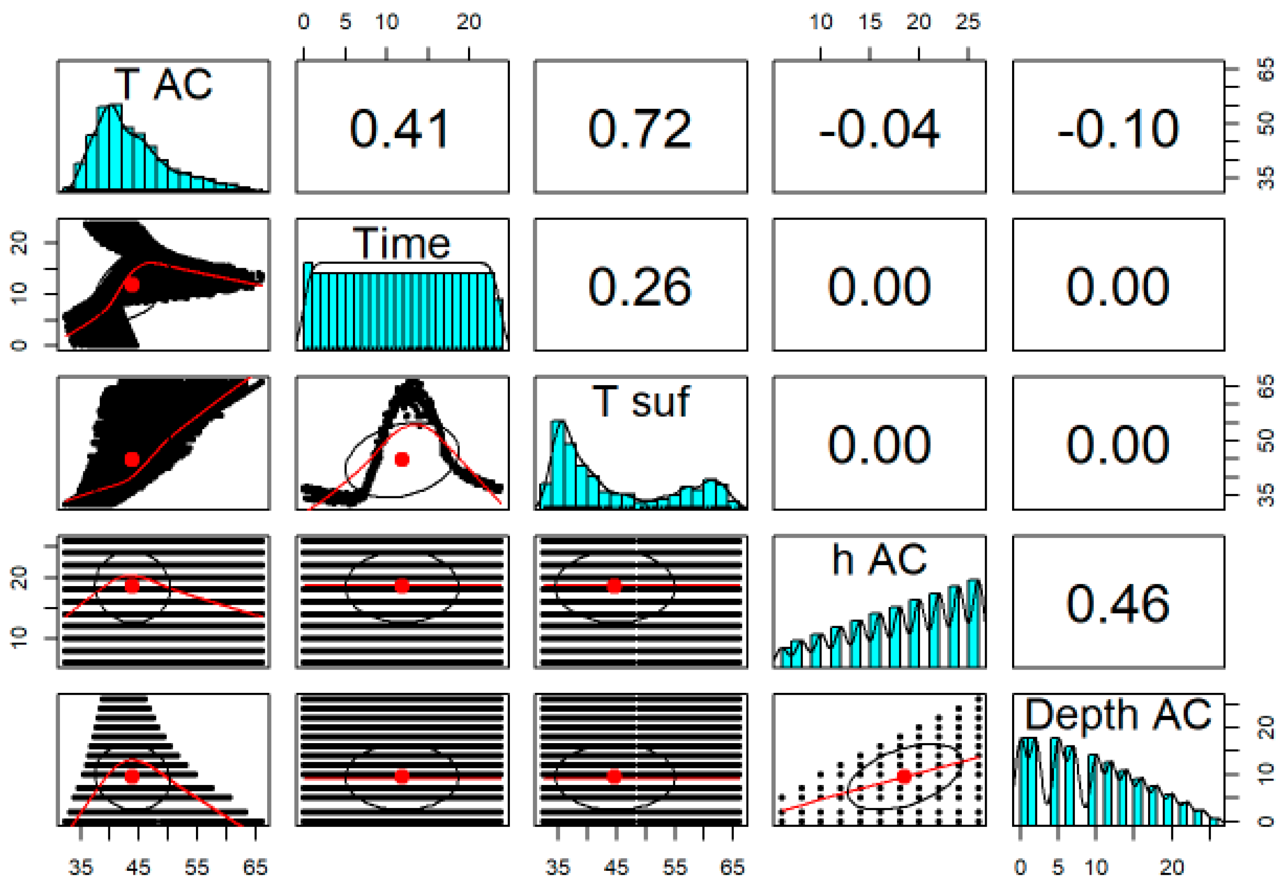
4.1. Correlation Analysis of Variables

For ANN model development to predict the temperature in AC, the AC temperature data were obtained from numerical simulations on semi-rigid pavements, in which variable-thickness AC layers were overlaid on CSB Dmax 31.5. The Pearson-based pair correlations between the AC temperature (T_AC, °C) and expected input variables were examined using the statistical analysis software R 4.2.1. These variables include the time of the day, surface temperature (T_suf, °C), AC thickness (h_AC, cm), and AC depth from the pavement surface (Depth_AC, cm). For the time of day (hours), values for half hours are presented as 0.5 h. For example, 15:30 is valued at 15.5 h. Time and depth help to determine the field temperature within AC across space and time. When using numerical methods, the paving surface temperature (T_suf) is the boundary domain for the heat transfer analysis. T_suf also works as a significant input for temperature prediction models, wherein changes in Tsuf result in positive changes in AC temperature (correlation of +0.72). Figure 8 demonstrates an inverse correlation between AC thickness and its temperature distribution. As the thickness of the AC increases, the temperature within the layer decreases. Although the variables h_AC and Depth_AC have a low correlation with T_AC, as analyzed and mentioned previously in Section 3, they are essential to accurately predict the temperature evolution in AC at each specific depth and thickness.

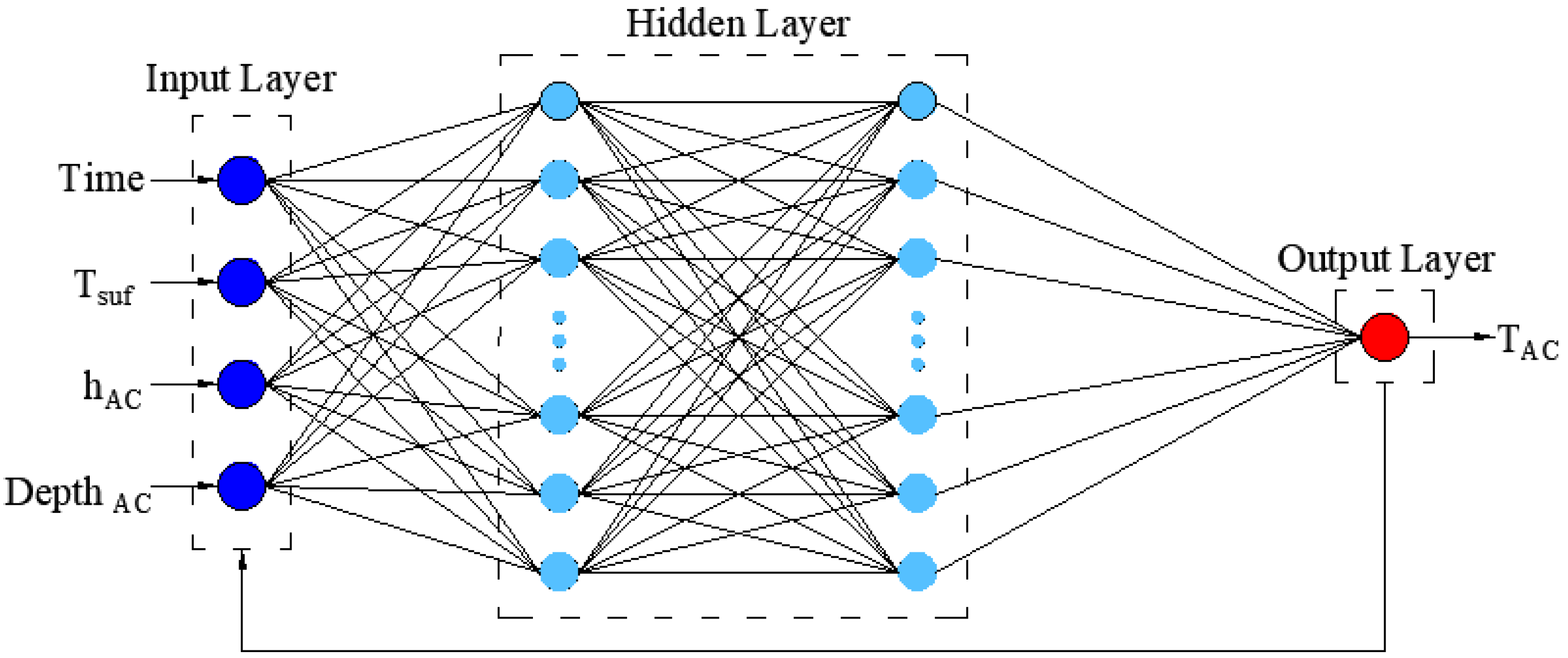
4.2. Development of ANN Model

The ANN consists of the input, hidden, and output layers. In this study, as illustrated in Figure 9, the input layer includes the following four parameters: the time of day (Time); surface temperature (T_suf); AC thickness (h_AC); and AC depth (Depth_AC). The output layer is a single variable of AC temperature (T_AC). Thao et al. [26] showed that a temperature distribution prediction model with two hidden layers resulted in the lowest amount of errors. Therefore, this study also used an ANN structure with two hidden layers; the neuron numbers in each layer varied from 10 to 20. The cascade-forward backpropagation network algorithm and the sigmoid non-linear transfer function were employed [26]. Initially, the output was computed by propagating input data from the input to the hidden layers. Subsequently, the error signal was obtained as the difference between the input and estimated data, which was then backpropagated from the output to the preceding layers to adjust the neural network weights.

In the ANN, the time of day (Time, h) has values changing from 0 to 24:00. The pavement surface temperature (T_suf, °C) was obtained through field temperature monitoring from 28 June to 2 July 2021, as reported by Tran et al. [18]. The temperature data at pavement depths of 2 cm, 5 cm, 7 cm, 10 cm, 12 cm, 14 cm, 16 cm, 18 cm, 20 cm, 22 cm, 24 cm, and 26 cm in the AC, with thicknesses ranging from 6 to 26 cm, were collected from the Ansys simulations at 10 min intervals for 11 different cases of varying AC thicknesses on a 15 cm CSB Dmax 25. These data were utilized to analyze and construct the ANN model.

Before the ANN model training, all input and output values were normalized within the [−1, 1] range. Out of the 62.832 temperature observations obtained from the Ansys-based numerical simulations, 70% were allocated for training, 15% for validation, and 15% for testing. Other parameters used for the training included a criterion error of 10⁻⁵ and a maximum number of iterations of 1000.

The optimized ANN model was selected based on the minor mean squared error (MSE), the most significant coefficient of determination (R), and the most considerable coefficient of determination (R²) (Figure 10, Figure 11 and Figure 12). It should be recalled that the temperature prediction model is applicable under rain-free weather conditions. Figure 11 and Figure 12 demonstrate the best predictive performance of the predicted model with two hidden layers, with 19 neurons in each, yielding an R of 0.998, an MSE of 0.000557, and an R² of 0.997.

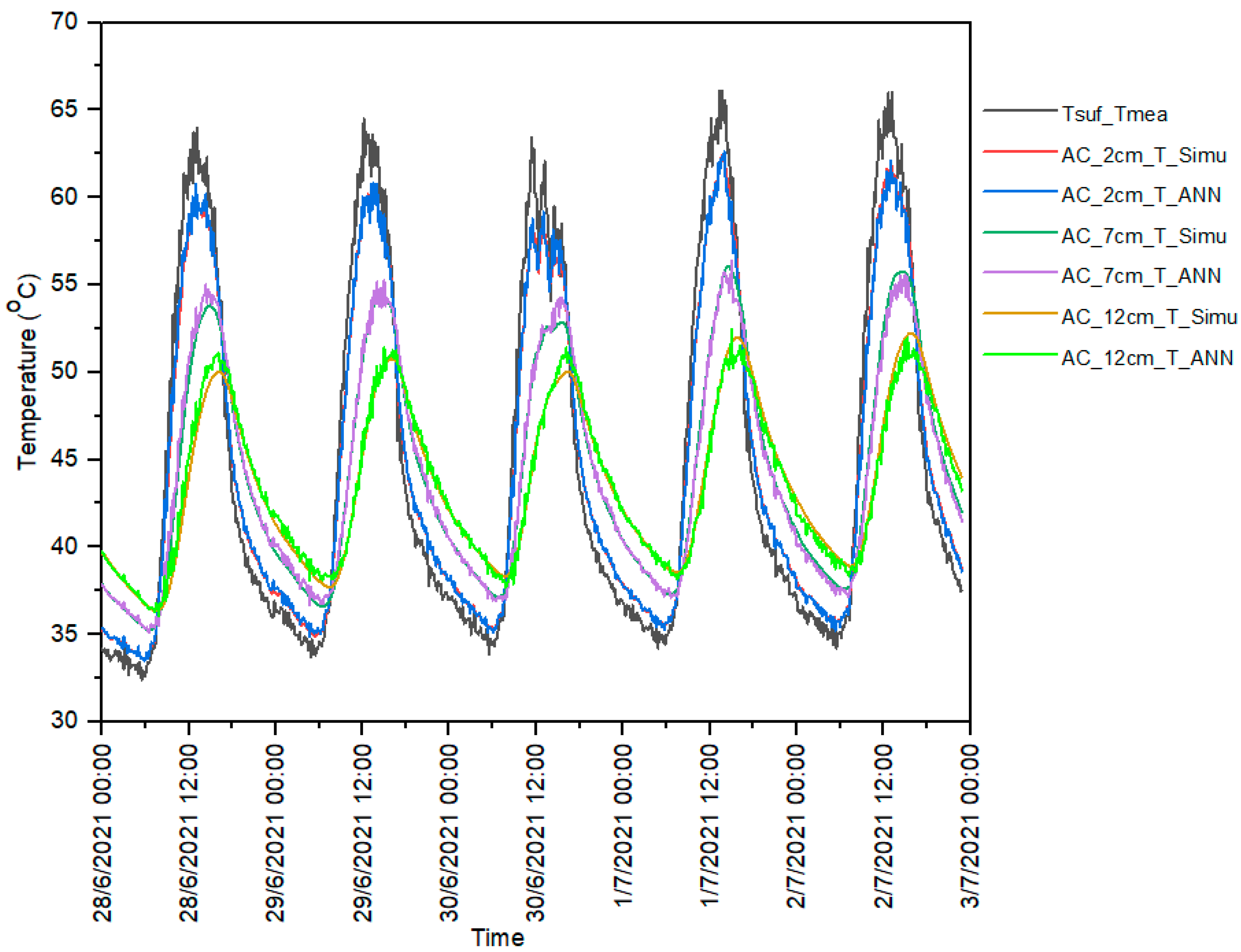
4.3. Temperature Prediction Comparison between ANN and Numerical Simulations

Figure 13 shows an identical temperature distribution at depths of 2 cm, 7 cm, and 12 cm within a 16 cm AC, as obtained from both the ANN prediction and numerical simulations.

To qualify the difference between the ANN prediction and the Ansys-based numerical simulations, the root mean square error (RMSE) of the temperature distribution was computed. The observed RMSE appears to be insignificant, at around 0.40 °C. The detailed RMSE for 11 different cases of varying AC thicknesses at depths of 2 cm, 5 cm, 7 cm, 10 cm, 12 cm, 14 cm, 16 cm, 18 cm, 20 cm, 22 cm, 24 cm, and 26 cm are presented in

Table 5. RMSE between the predicted temperature from the numerical simulation and ANN model.

AC Depth (cm)	RMSE of AC Temperature (°C) between Numerical Simulation and ANN for Each AC Layer Thickness (cm)
	6	8	10	12	14	16	18	20	22	24	26
0	0.35	0.33	0.33	0.33	0.33	0.33	0.33	0.33	0.33	0.34	0.34
2	0.30	0.29	0.28	0.28	0.28	0.28	0.28	0.28	0.28	0.39	0.38
5	0.35	0.34	0.34	0.34	0.33	0.33	0.33	0.33	0.33	0.33	0.33
7	-	0.39	0.37	0.36	0.36	0.36	0.36	0.35	0.35	0.34	0.34
10	-	-	0.42	0.41	0.40	0.40	0.40	0.39	0.38	0.37	0.37
12	-	-	-	0.44	0.43	0.43	0.42	0.41	0.40	0.39	0.39
14	-	-	-	-	0.46	0.46	0.45	0.44	0.42	0.41	0.41
16	-	-	-	-	-	0.48	0.47	0.46	0.44	0.43	0.67
18	-	-	-	-	-	-	0.49	0.48	0.46	0.44	0.44
20	-	-	-	-	-	-	-	0.50	0.48	0.46	0.45
22	-	-	-	-	-	-	-	-	0.50	0.47	0.47
24	-	-	-	-	-	-	-	-	-	0.49	0.48
26	-	-	-	-	-	-	-	-	-	-	0.50

. The findings reveal the suitability of the proposed ANN model compared with the numerical simulations, confirmed by the acceptable RMSE, ranging from 0.28 °C to 0.67 °C. Abo-Hashema [37] also used ANN to predict the AC temperature based on air and pavement surface temperatures. His suggested ANN model showed that the standard error of estimate (SEE) = 1.3 °C and R = 0.985. In this study, the proposed ANN has more advantages than Abo-Hashema’s model [37], with a lower SEE and higher R, which significantly helps to better estimate temperatures for various AC thicknesses.

The temperature estimation from the numerical simulation, and especially from the developed ANN model, can be used in the following applications:

(i)

Selecting appropriate AC properties for pavement analysis and design;

(ii)

Estimating the depth AC temperature used to test the modulus of elasticity of semi-rigid pavements using the falling weight deflectometer test;

(iii)

Finding a way to reduce temperature distribution in summer seasons;

(iv)

Analyzing the long-term performance of pavements.

5. Conclusions

This study investigated temperature distribution in the AC with thicknesses ranging from 6 cm to 26 cm on CSB using different granular gradations (Dmax 25 and Dmax 31.5) and incorporating RA (3–6 mm) as a partial replacement for the graded aggregates, by volume, in Dmax 25. From the numerical simulation and the ANN model, some main conclusions can be drawn, as follows:

• CSB gradation influences temperature distributions in semi-rigid pavement structures. CSB Dmax 31.5, with a higher density than CSB Dmax 25, resulted in lower temperature fluctuations at the bottom of the AC, of around 8%. It also led to negligible temperature variations between the AC top and bottom, of less than 5.5%;
• Incorporating RA in CSB Dmax 25 reduced the temperature distribution within the AC. Primarily, a 5% addition of RA resulted in up to a 20.4% reduction in temperature fluctuation at the AC bottom. A slight increase in the temperature difference between the top and bottom of the AC was observed when RA was used; however, these changes were insignificant for semi-rigid pavement structures with an hAC exceeding 12 cm;
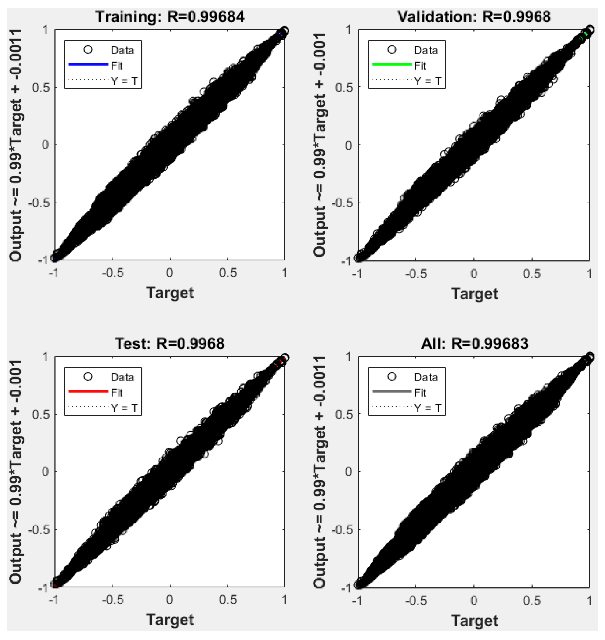
• The proposed ANN model with four inputs, including the time of day, pavement surface temperature, AC thickness, and depth, was adopted to predict the temperature in the AC of semi-rigid pavements, was confirmed by the Ansys-based numerical simulations. This model was applied in free-rain conditions with a pavement surface temperature range of 32.4 °C ÷ 66.1 °C and an AC thickness varying from 6 cm to 26 cm. The proposed model, confirmed by the numerical simulations, exhibited high accuracy (R² = 0.996 and MSE = 0.000685).

Due to the benefit of rubberized CSB, potential studies should focus on its practical application in semi-rigid pavements. Then, actual field temperature monitoring could be obtained and compared with the developed numerical simulations and the ANN model.

References

1. Xuan, D.X.; Molenaar, A.A.A.; Houben, L.J.M. Shrinkage Cracking of Cement Treated Demolition Waste as a Road Base. Mater. Struct. Constr. 2016, 49, 631–640. [Google Scholar] [CrossRef]
2. Mohammadinia, A.; Arulrajah, A.; Sanjayan, J.; Disfani, M.M.; Win Bo, M.; Darmawan, S. Stabilization of Demolition Materials for Pavement Base/Subbase Applications Using Fly Ash and Slag Geopolymers: Laboratory Investigation. J. Mater. Civ. Eng. 2016, 28, 04016033. [Google Scholar] [CrossRef]
3. Gnanendran, C.T.; Paul, D.K. Fatigue Characterization of Lightly Cementitiously Stabilized Granular Base Materials Using Flexural Testing. J. Mater. Civ. Eng. 2016, 28, 04016086. [Google Scholar] [CrossRef]
4. Mráz, V.; Valentin, J.; Suda, J.; Kopecký, L. Experimental Assessment of Fly-Ash Stabilized and Recycled Mixes. J. Test. Eval. 2015, 43, 264–278. [Google Scholar] [CrossRef]
5. Lv, S.; Xia, C.; Liu, H.; You, L.; Qu, F.; Zhong, W.; Yang, Y.; Washko, S. Strength and Fatigue Performance for Cement-Treated Aggregate Base Materials. Int. J. Pavement Eng. 2019, 22, 690–699. [Google Scholar] [CrossRef]
6. Adaska, W.S.; Luhr, D.R. Control of Reflective Cracking in Cement Stabilized Pavements. In Proceedings of the 5th International RILEM Conference, Limoges, France, 5 May 2004; Volume 2, pp. 1–8. [Google Scholar]
7. Farhan, A.H.; Dawson, A.R.; Thom, N.H.; Adam, S.; Smith, M.J. Flexural Characteristics of Rubberized Cement-Stabilized Crushed Aggregate for Pavement Structure. Mater. Des. 2015, 88, 897–905. [Google Scholar] [CrossRef]
8. Liu, L.; Wang, C.; Liang, Q.; Chen, F.; Zhou, X. A State-of-the-Art Review of Rubber Modified Cement-Based Materials: Cement Stabilized Base. J. Clean. Prod. 2023, 392, 136270. [Google Scholar] [CrossRef]
9. Pham, P.N.; Tran, T.T.T.; Nguyen, P.; Truong, T.A.; Siddique, R. Rubberized Cement-Stabilized Aggregates: Mechanical Performance, Thermal Properties, and Effect on Temperature Fluctuation in Road Pavements. Transp. Geotech. 2023, 40, 100982. [Google Scholar] [CrossRef]
10. Tran, T.T.T.; Nguyen, H.H.; Pham, P.N.; Nguyen, T.; Phuc, Q.; Huynh, H.N. Temperature-Related Thermal Properties of Paving Materials: Experimental Analysis and Effect on Thermal Distribution in Semi-Rigid Pavement. Road Mater. Pavement Des. 2023, 24, 2759–2779. [Google Scholar] [CrossRef]
11. Joumblat, R.; Kassem, H.A.; Al Basiouni Al Masri, Z.; Elkordi, A.; Al-Khateeb, G.; Absi, J. Performance Evaluation of Hot-Mix Asphalt with Municipal Solid Waste Incineration Fly Ash Using the Stress Sweep Rutting Test. Innov. Infrastruct. Solut. 2023, 8, 261. [Google Scholar] [CrossRef]
12. Duan, W.; Zhuge, Y.; Pham, P.N.; Chow, C.W.K.; Keegan, A.; Liu, Y. Utilization of Drinking Water Treatment Sludge as Cement Replacement to Mitigate Alkali–Silica Reaction in Cement Composites. J. Compos. Sci. 2020, 4, 171. [Google Scholar] [CrossRef]
13. Gu, L.; Liu, Y.; Zeng, J.; Zhang, Z.; Pham, P.N.; Liu, C. The Synergistic Effects of Fibres on Mechanical Properties of Recycled Aggregate Concrete: A Comprehensive Review. Constr. Build. Mater. 2024, 436, 137011. [Google Scholar] [CrossRef]
14. Ferretti, E.; Bignozzi, M.C. Stress and Strain Profiles along the Cross-Section of Waste Tire Rubberized Concrete Plates for Airport Pavements. Comput. Mater. Contin. 2012, 27, 231–273. [Google Scholar] [CrossRef]
15. Bayraktarova, K.; Eberhardsteiner, L.; Zhou, D.; Blab, R. Characterisation of the Climatic Temperature Variations in the Design of Rigid Pavements. Int. J. Pavement Eng. 2022, 23, 3222–3235. [Google Scholar] [CrossRef]
16. Gui, J.G.; Carlson, J.; Phelan, P.E.; Kaloush, K.E.; Golden, J.S. Impact of Pavement Thermophysical Properties on Surface Temperatures. J. Mater. Civ. Eng. 2007, 2, 683–690. [Google Scholar] [CrossRef]
17. Fujimato, A.; Saida, A.; Fukuhara, T. A New Approach to Modeling Vehicle-Induced Heat and Its Thermal Effects on Road Surface Temperature. J. Appl. Meteorol. Climatol. 2012, 51, 1980–1993. [Google Scholar] [CrossRef]
18. Tran, T.T.T.; Nguyen, H.H.; Pham, P.N.; Nguyen, P.Q. Effect of Asphalt Concrete Layer Thickness on Temperature Distribution in the Semi-Rigid Pavement. In Proceedings of the IOP Conference Series: Materials Science and Engineering, the 4th International Conference on Transportation Infrastructure and Sustainable Development (TISDIC-2023), Danang, Vietnam, 26–28 August 2023; IOP Publishing: Bristol, UK, 2023; Volume 1289, p. 12060. [Google Scholar]
19. Côté, J.; Konrad, J.M. Thermal Conductivity of Base-Course Materials. Can. Geotech. J. 2005, 42, 61–78. [Google Scholar] [CrossRef]
20. Gong, X.; Liu, Q.; Lv, Y.; Chen, S.; Wu, S.; Ying, H. A Systematic Review on the Strategies of Reducing Asphalt Pavement Temperature. Case Stud. Constr. Mater. 2023, 18, e01852. [Google Scholar] [CrossRef]
21. Mirzanamadi, R.; Johansson, P.; Grammatikos, S.A. Thermal Properties of Asphalt Concrete: A Numerical and Experimental Study. Constr. Build. Mater. 2018, 158, 774–785. [Google Scholar] [CrossRef]
22. Hassn, A.; Aboufoul, M.; Wu, Y.; Dawson, A.; Garcia, A. Effect of Air Voids Content on Thermal Properties of Asphalt Mixtures. Constr. Build. Mater. 2016, 115, 327–335. [Google Scholar] [CrossRef]
23. Yan, X.; Chen, L.; You, Q.; Fu, Q. Experimental Analysis of Thermal Conductivity of Semi-Rigid Base Asphalt Pavement. Road Mater. Pavement Des. 2019, 20, 1215–1227. [Google Scholar] [CrossRef]
24. Merhebi, G.H.; Joumblat, R.; Elkordi, A. Assessment of the Effect of Different Loading Combinations Due to Truck Platooning and Autonomous Vehicles on the Performance of Asphalt Pavement. Sustainability 2023, 15, 10805. [Google Scholar] [CrossRef]
25. TCCS 38:2022/TCDBVN; Flexible Pavement Design-Specification and Guidelines. Vietnamese Stand: Hanoi, Vietnam, 2022.
26. Tran, T.T.T.; Pham, P.N.; Nguyen, H.H.; Nguyen, P.Q. Prediction of Temperature Distribution in Cement—Treated Bases Considering the Influence of Rubber Aggregates and Asphalt Layer Thickness. Transp. Commun. Sci. J. 2023, 74, 1002–1016. [Google Scholar] [CrossRef]
27. Adwan, I.; Milad, A.; Memon, Z.A.; Widyatmoko, I.; Zanuri, N.A.; Memon, N.A.; Yusoff, N.I.M. Asphalt Pavement Temperature Prediction Models: A Review. Appl. Sci. 2021, 11, 3794. [Google Scholar] [CrossRef]
28. Wang, D. Analytical Approach to Predict Temperature Profile in a Multilayered Pavement System Based on Measured Surface Temperature Data. J. Transp. Eng. 2012, 138, 674–679. [Google Scholar] [CrossRef]
29. Molavi Nojumi, M.; Huang, Y.; Hashemian, L.; Bayat, A. Application of Machine Learning for Temperature Prediction in a Test Road in Alberta. Int. J. Pavement Res. Technol. 2022, 15, 303–319. [Google Scholar] [CrossRef]
30. Matić, B.; Matić, D.; Sremac, S.; Radović, N.; Viđikant, P. A Model for The Pavement Temperature Prediction At Specified Depth Using Neural Networks. Metalurgija 2013, 53, 665–667. [Google Scholar]
31. Najafi, Z.; Ahangari, K. The Prediction of Concrete Temperature during Curing Using Regression and Artificial Neural Network. J. Eng. 2013, 2013, 946829. [Google Scholar] [CrossRef]
32. Qin, Y.; Hiller, J.E. Modeling Temperature Distribution in Rigid Pavement Slabs: Impact of Air Temperature. Constr. Build. Mater. 2011, 25, 3753–3761. [Google Scholar] [CrossRef]
33. Sun, L. Structural Behavior of Asphalt Pavements; Elsevier: Amsterdam, The Netherlands, 2016; ISBN 978-0-12-849908-5. [Google Scholar]
34. Chen, J.; Wang, H.; Xie, P. Pavement Temperature Prediction: Theoretical Models and Critical Affecting Factors. Appl. Therm. Eng. 2019, 158, 113755. [Google Scholar] [CrossRef]
35. Minhoto, M.J.C.; Pais, J.C.; Pereira, P.A.A. Asphalt Pavement Temperature Prediction. In Proceedings of the Asphalt Rubber Conference, Palm Springs, CA, USA, October 2006; pp. 193–207. [Google Scholar]
36. Zhang, L.; Wang, H.; Ren, Z. Computational Analysis of Thermal Conductivity of Asphalt Mixture Using Virtually Generated Three-Dimensional Microstructure. J. Mater. Civ. Eng. 2017, 29, 04017234. [Google Scholar] [CrossRef]
37. Abo-Hashema, M.A. Modeling Pavement Temperature Prediction Using Artificial Neural Networks. In Proceedings of the Airfield and Highway Pavement 2013: Sustainable and Efficient Pavements—Proceedings of the 2013 Airfield and Highway Pavement Conference, Los Angeles, CA, USA, 9–12 June 2013; pp. 490–505. [Google Scholar]
38. Available online: https://www.ansys.com/training-center/course-catalog/structures/introduction-to-ansys-workbench (accessed on 1 August 2023).
39. Minhoto, M.J.C.; Pais, J.C.; Pereira, P.A.A.; Picado-santos, L.G. Predicting Asphalt Pavement Temperature with a Three-Dimensional Finite Element Method. Transp. Res. Rec. 2005, 1919, 96–110. [Google Scholar] [CrossRef]
40. Zhang, N.; Wu, G.; Chen, B.; Cao, C. Numerical Model for Calculating the Unstable State Temperature in Asphalt Pavement Structure. Coatings 2019, 9, 271. [Google Scholar] [CrossRef]
41. Alavi, M.Z.; Pouranian, M.R.; Hajj, E.Y. Prediction of Asphalt Pavement Temperature Profile with Finite Control Volume Method. Transp. Res. Rec. 2014, 2456, 96–106. [Google Scholar] [CrossRef]
42. Mammeri, A.; Ulmet, L.; Peti, C.; Mokhtari, A.M. Temperature Modelling in Pavements: The Effect of Long-and Short-Wave Radiation. Int. J. Pavement Eng. 2015, 16, 198–213. [Google Scholar] [CrossRef]
Figure 1. Simulation steps of thermal distribution in road pavements using Ansys 2023 R2.
Buildings 14 02470 g001
Figure 2. Temperature distribution at the moment of peak temperature at the bottom of the AC.
Buildings 14 02470 g002
Figure 3. Temperature fluctuation at the AC bottom versus AC thickness as CSB Dmax 25 and CSB Dmax 31.5 were used.
Buildings 14 02470 g003
Figure 4. Temperature variation between the bottom and top of AC versus AC thicknesses in two cases of CSB Dmax 25 and CSB Dmax 31.5.
Buildings 14 02470 g004
Figure 5. Temperature distribution at the moment of peak temperature at the bottom of AC with varying AC thickness and RA in CSB Dmax 25.
Buildings 14 02470 g005
Figure 6. Temperature variation at AC bottom versus AC thickness in CSB Dmax 25 incorporating different RA contents.
Buildings 14 02470 g006
Figure 7. Temperature variation between the bottom and top of AC versus AC thicknesses in case CSB Dmax 25 incorporating different RA contents.
Buildings 14 02470 g007
Figure 8. Correlation analysis between AC temperature and input variables by R 4.2.1.
Buildings 14 02470 g008
Figure 9. ANN structure.
Buildings 14 02470 g009
Figure 10. Training observation with 11 neurons in hidden layers.
Buildings 14 02470 g010
Figure 11. MSE and R versus hidden layer neuron.
Buildings 14 02470 g011
Figure 12. Hidden layer neuron versus R2.
Buildings 14 02470 g012
Figure 13. Temperature evolution in a 16 cm AC at depths of 2 cm, 7 cm, and 12 cm from the ANN model and numerical simulation.
Buildings 14 02470 g013