

Achieving Financial Feasibility and Carbon Emission Reduction: Retrofit of a Bangkok Shopping Mall Using Calibrated Simulation

Abstract
:1. Introduction
2. Materials and Methods
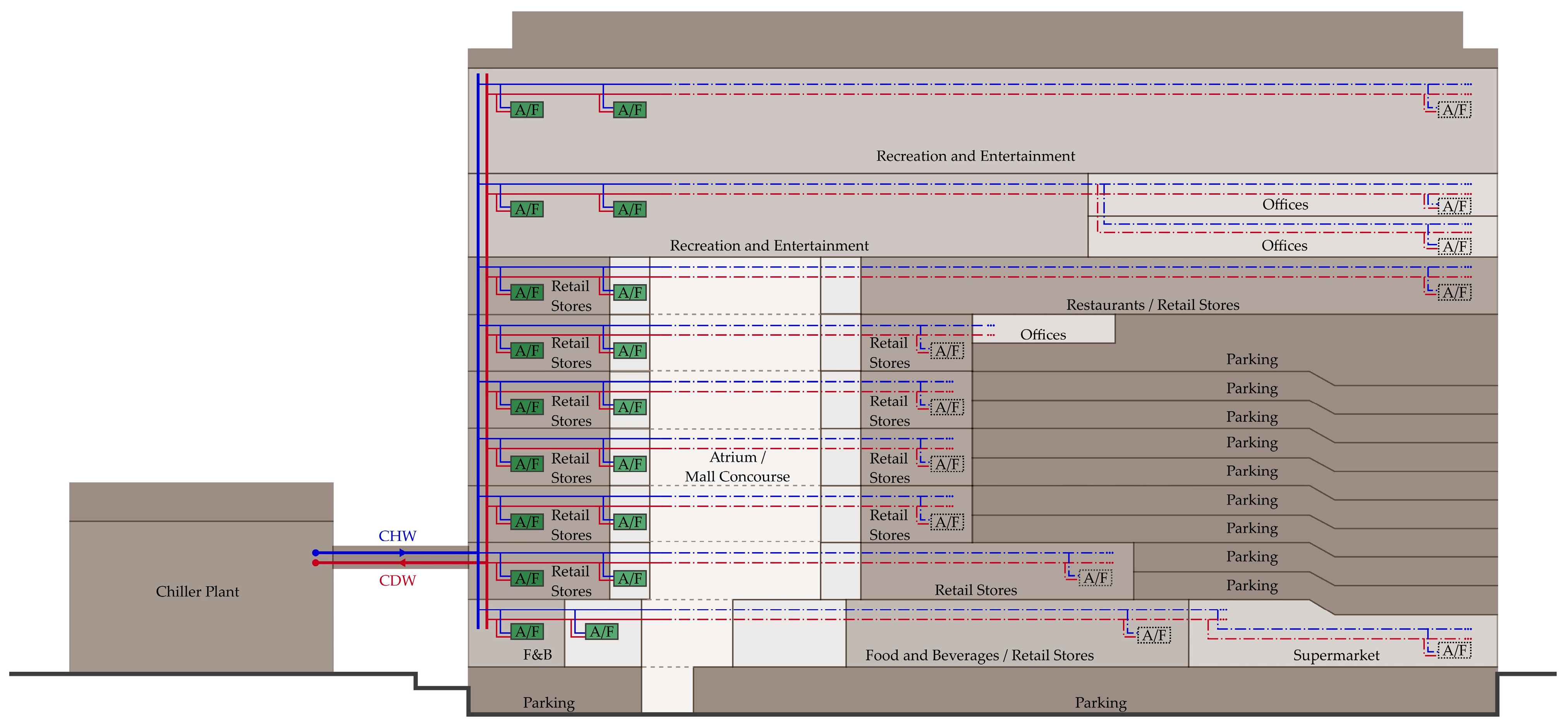
2.1. Case Study Building
2.2. Building Energy Modeling
2.2.1. Reference Model
- Normalized mean bias error (NMBE) is a statistical indicator used to assess a model’s tendency to under-predict or over-predict actual consumption data during the evaluation period. A positive NMBE indicates underestimation, whereas a negative NMBE signifies overestimation. The NMBE is expressed as a percentage (%) and is calculated as shown in Equation (1).
- Coefficient of variance of the root mean square error (CVRMSE) is a statistical indicator used to assess the relative magnitude of the errors between simulated and measured monthly energy consumption data. A lower CVRMSE value indicates better agreement between the model and the building’s actual performance. CVRMSE is expressed as a percentage (%) and is calculated as shown in Equation (2).where
= measured energy use for each month; = simulated energy use for each month; = arithmetic mean of the measured data; = interval that the measured and simulated data are aligned to; = number of intervals (greater than 1) included in the analysis; = 1.
2.2.2. Proposed Model
2.3. Economic Analysis
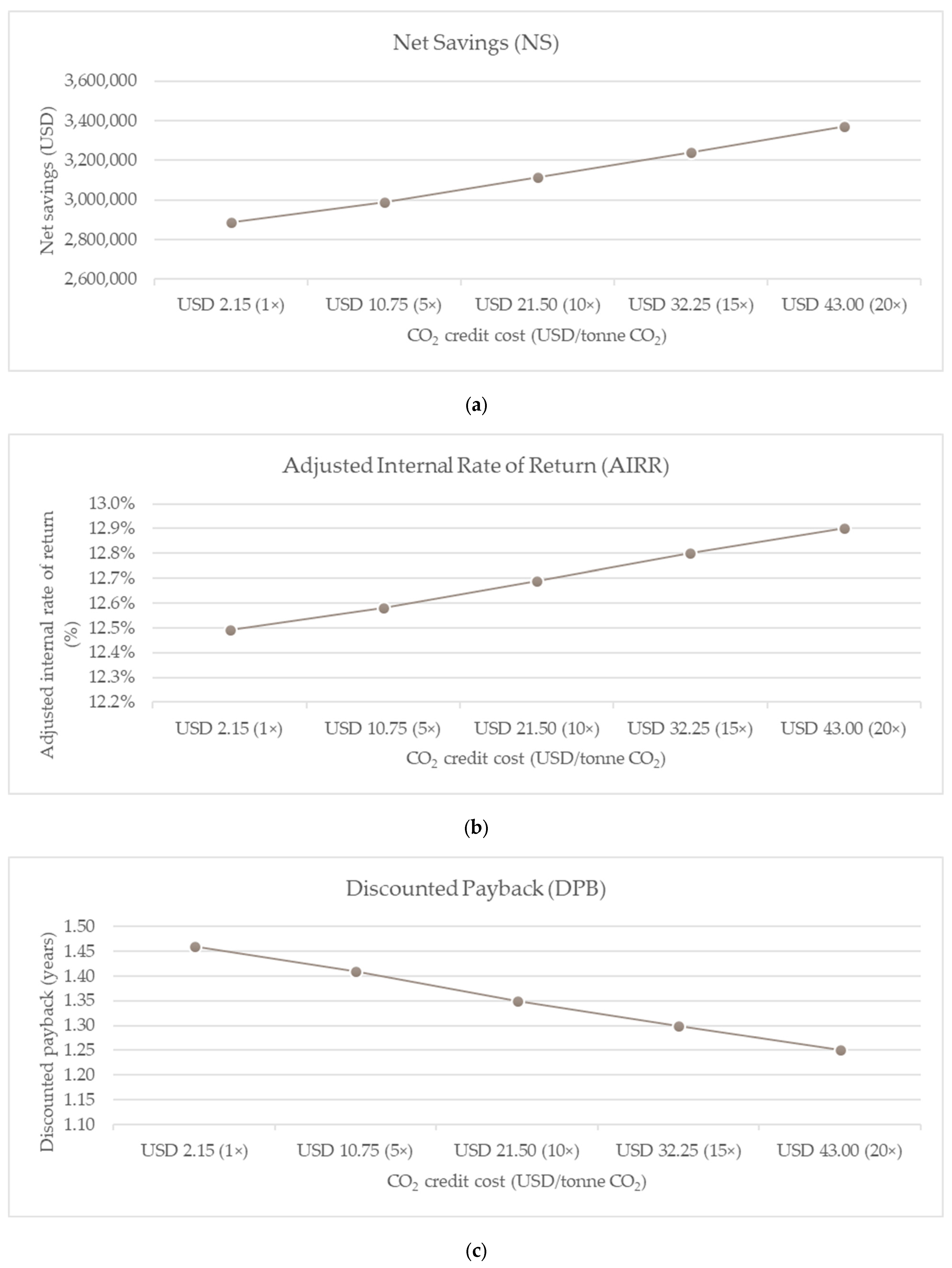
- Net savings (NS): This metric represents the net financial benefit of an ECM over its lifetime. It considers the present value of all cost savings generated by the ECM (e.g., reduced energy costs) minus the present value of all costs incurred (e.g., installation and maintenance costs). A positive NS value indicates a financially beneficial ECM. Equation (3) defines the NS calculation.
- Adjusted internal rate of return (AIRR): This measure reflects the discount rate at which the net present value of an ECM’s cash flow is zero. A higher AIRR indicates a more financially attractive ECM compared to alternative investments with a lower AIRR. Equations (4) and (5) provide the calculations of the AIRR.
- Discounted payback period (DPB): This metric represents the time it takes for the cumulative net cash flow from an ECM (i.e., cost savings minus costs) to equal the initial investment cost. A shorter DPB indicates a faster financial return on the investment. Equation (6) presents the formula for calculating the DPB.where
= NS, in PV dollars, of alternative (A), relative to base case (BC); = saving-to-investment ratio; = SIR of alternative (A) relative to base case (BC); = initial investment costs associated with the alternative; = additional investment-related costs in year t associated with the alternative; = savings in year t in operational costs associated with the alternative; = reinvestment rate; = discounted rate; = number of years in study period; = minimum length of time over which future net cash flows have to be accumulated in order to offset initial investment costs; = year of occurrence (where 0 is the base date).
- Number of analysis years: NIST Handbook 135 recommends a maximum lifespan of 40 years for buildings in economic analyses. Considering that the shopping mall has been operational for five years, the study adopted a 35-year analysis period.
- Discount rate and MIRR: A discount rate and MIRR of 7% were assumed. This value aligns with commercial lending rates in Thailand, reflecting the financial conditions relevant to the shopping mall project. It is also consistent with the rate used by Seeley and Dhakal (2021) in a similar study [5].
- Escalation rate: The electricity price escalation rate of 1% published by the DEDE was adopted. Since this rate has been in effect for over ten years, a sensitivity analysis was conducted using escalation rates of 2% and 3% to assess the impact of this variable on the analysis results.
- CO2 emission factor: The CO2 emission factor as of 2023 that was used in this study is 0.44 kgCO2e per kilowatt-hour of electricity consumption, which was published by the Energy Policy and Planning Office (EPPO) [38].
3. Results
3.1. Building Energy Modeling and Simulation Results
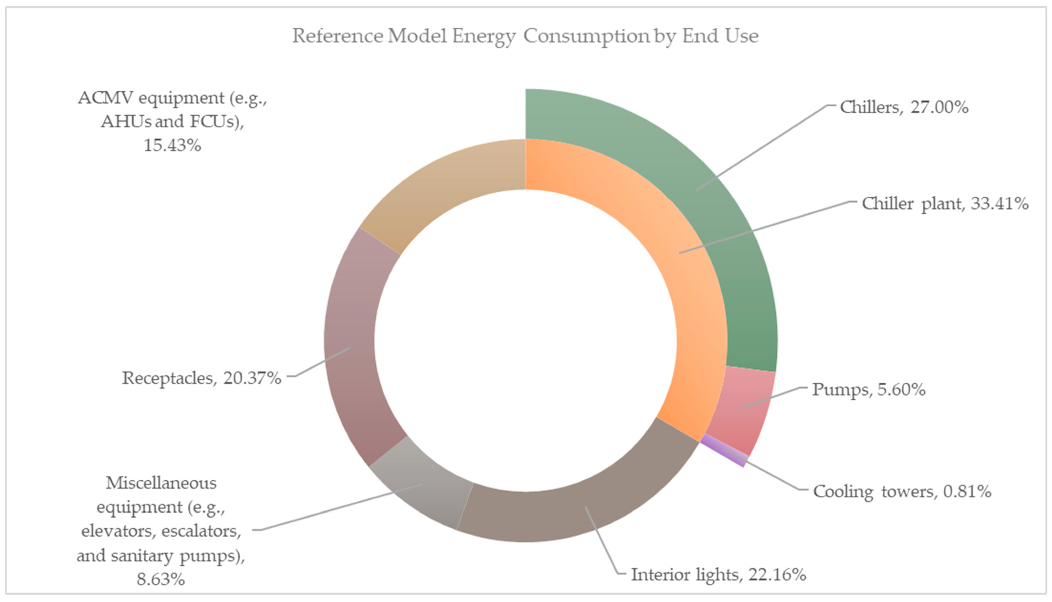
3.1.1. Reference Model Results
3.1.2. Proposed Model Results
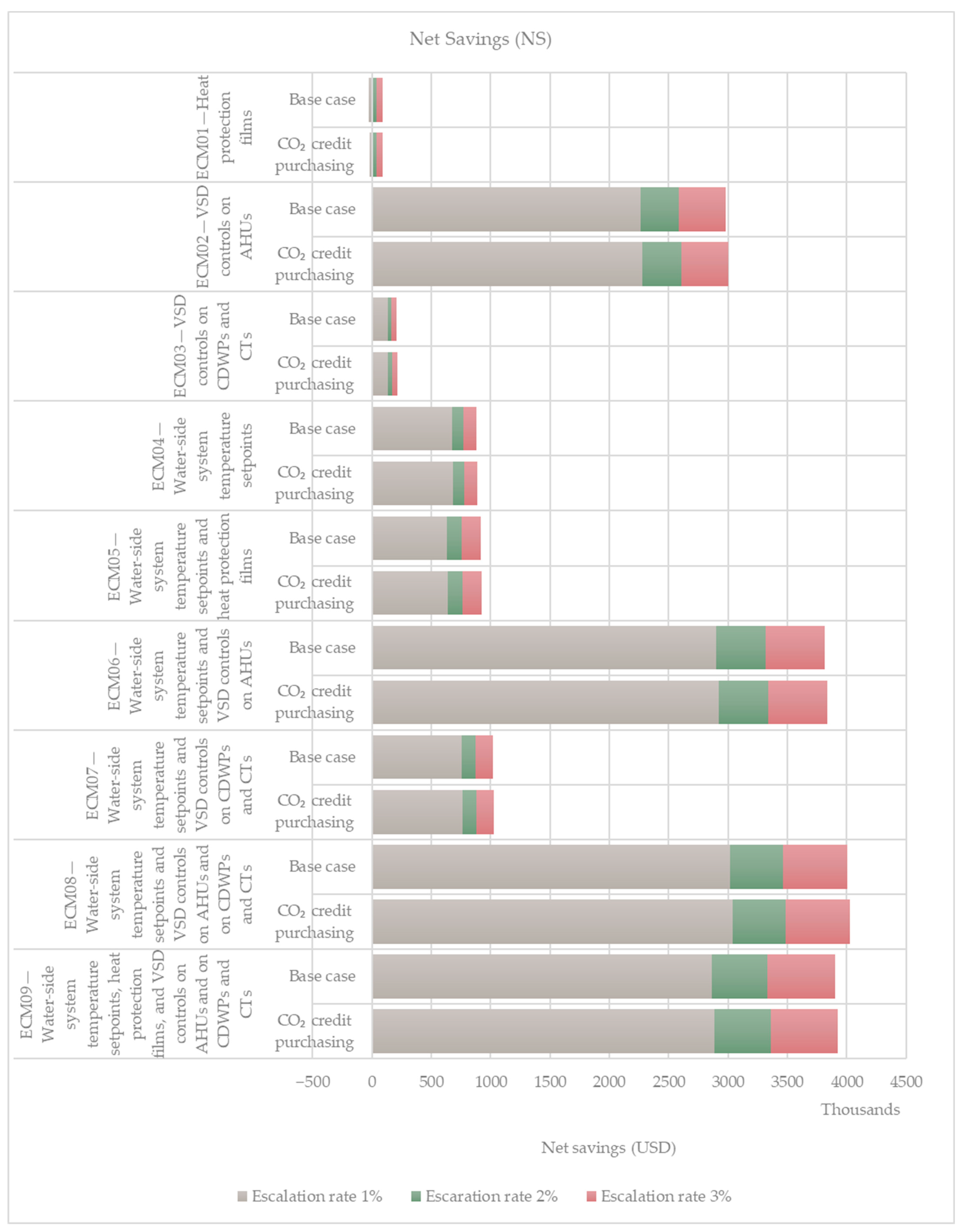
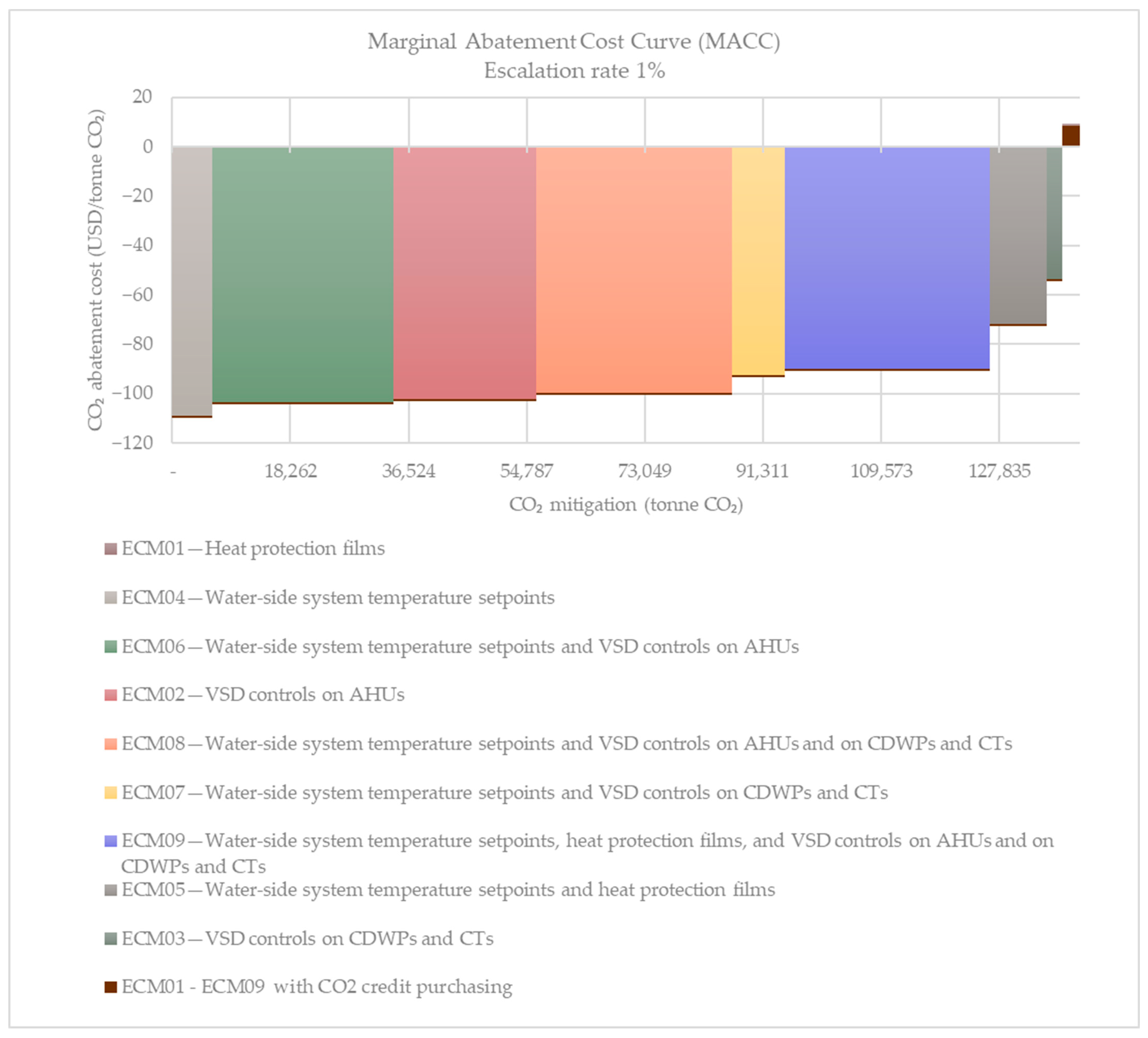
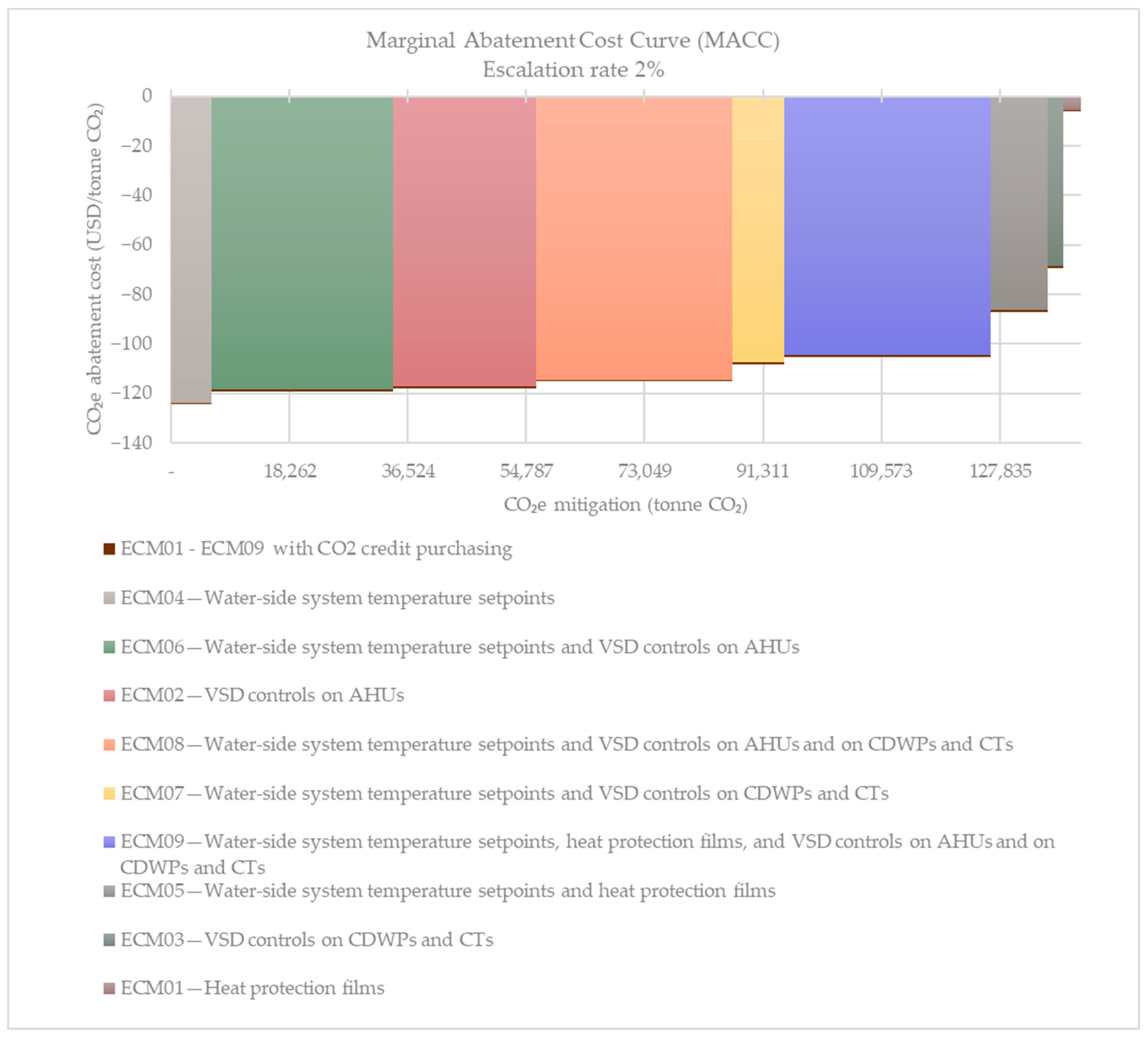
3.2. Economic Analysis Results
4. Discussion
- Building envelope: Strategies to reduce solar heat gain through the building envelope were explored.
- ACMV system equipment: Measures to enhance the efficiency of the ACMV system equipment were investigated.
- Chilled water plant equipment: Optimization strategies for the chilled water plant equipment were evaluated.
- Chilled and condenser water settings: The potential benefits of adjusting the chilled and condenser water settings were analyzed.
- Accurate building information is crucial for developing a reference model. For this study, valid information for energy modeling can be obtained for a building that has been operational for five years. However, for older buildings, the availability of accurate information may be limited, leading to the need for modeling assumptions and software defaults. This, in turn, may result in a discrepancy between the simulated and actual energy use of the building [11].
- Independent variables, particularly weather and occupancy data, are critical during model calibration. We strongly suggest utilizing the AMY weather data for this purpose. Occupancy data are also important but can be among the most uncertain inputs [11]. In this project, occupancy data significantly accelerated the calibration process.
- Multiple-objective calibration is essential for achieving a well-calibrated model. Focusing solely on fine-tuning the model with a single objective, such as matching only the monthly energy consumption and demand, may not be sufficient. In our recent study, examining various aspects of energy use, including chiller plant energy consumption and capacity data, was crucial for effective calibration.
- Metering data are vital for model calibration. However, the limitations in the building’s energy monitoring system hindered our ability to collect detailed data on specific end uses like lighting. If feasible, advanced metering infrastructure could be a valuable investment for new buildings to facilitate more comprehensive data collection for future modeling efforts [41].
- Model calibration methods deserve further exploration. Using an expert knowledge method for model calibration heavily relies on the modeler’s knowledge and judgement. This approach can be time-consuming and may not yield consistent results for future projects. To address this, we concur with previous literature, like Reddy (2006), that emphasizes the need for replicable procedural methods to improve the model calibration process [9,10,11,12]. This area warrants further investigation in future studies.
- Conduct a preliminary energy audit: Assess the building’s current energy performance to understand its energy use characteristics and identify potential areas for energy savings.
- Develop a calibrated energy model: Gather and use building information, independent variables, and historical energy use data to create a calibrated energy model of the building. This model will be critical for evaluating the impact of different ECMs.
- Evaluate ECMs: Identify and analyze various ECMs using the calibrated energy model. Consider factors such as energy savings, costs, and implementation practicality.
- Perform economic analysis: Conduct a detailed economic analysis considering financial variables such as electricity escalation rates, carbon credit prices, and potential incentives. Assess the NS, AIRR, DPB, or other economic indicators of interest for each ECM.
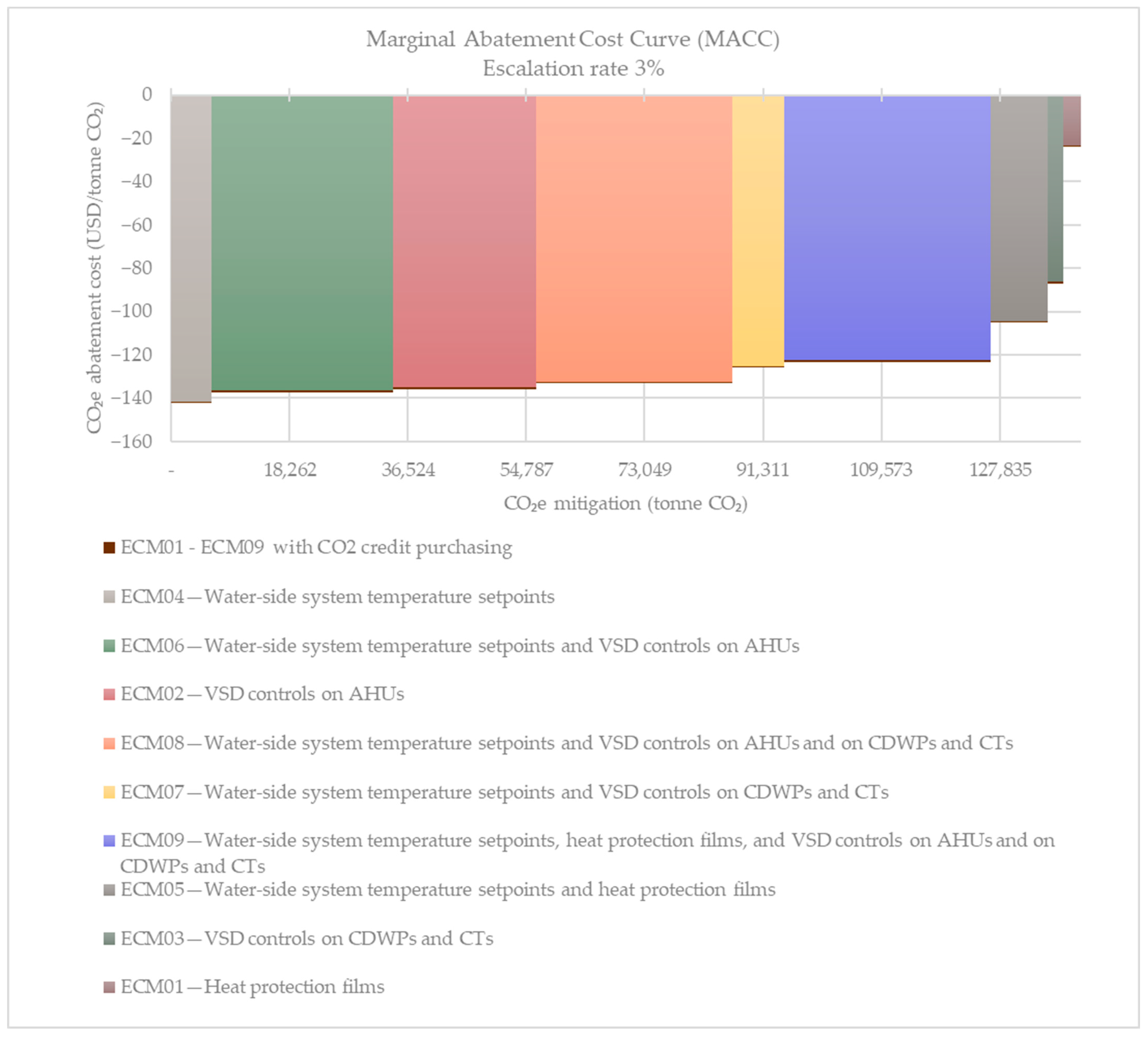
- Prioritize ECMs: Based on the energy and economic analysis, prioritize ECMs that offer the highest energy savings, environmental benefits, and financial returns. The MACC is a valuable tool for prioritizing the ECMs.
- Develop an implementation plan: Create a detailed plan for implementing the selected ECMs, including timeframe, budget, and resource allocation.
- Monitor and verify performance: After implementation, continuously monitor the building’s energy performance and compare it with the expected outcomes to ensure that the ECMs deliver the anticipated benefits.
5. Conclusions
Author Contributions
Funding
Data Availability Statement
Acknowledgments
Conflicts of Interest
References
- Thailand. Thailand’s 2nd Updated Nationally Determined Contribution; The United Nations Framework on Climate Change: Bonn, Germany, 2022; Available online: https://unfccc.int/documents/620602 (accessed on 17 April 2024).
- United Nations Environment Programme; Global Alliance for Buildings and Construction. 2023 Global Status Report for Buildings and Construction: Beyond Foundations—Mainstreaming Sustainable Solutions to cut Emissions from the Buildings Sector; UN Environment Programme: Nairobi, Kenya, 2024. [Google Scholar] [CrossRef]
- Ministry of Energy Thailand. Energy Statistics of Thailand 2023; Department of Alternative Energy Development and Efficiency (DEDE), Ministry of Energy Thailand Publications: Bangkok, Thailand, 2023.
- Knight Frank Thailand. An Overview Review of Bangkok’s Retail Market in Mid-2023; Knight Frank: Bangkok, Thailand, 2023; Available online: https://www.knightfrank.co.th/research (accessed on 17 April 2024).
- Seeley, C.C.; Dhakal, S. Energy efficiency retrofits in Commercial buildings: An environmental, financial, and technical analysis of case studies in Thailand. Energies 2021, 14, 2571. [Google Scholar] [CrossRef]
- Augenbroe, G. Trends in building simulation. Build. Environ. 2002, 37, 891–902. [Google Scholar] [CrossRef]
- Yuan, J.; Nian, V.; Su, B.; Meng, Q. A simultaneous calibration and parameter ranking method for building energy models. Appl. Energy 2017, 206, 657–666. [Google Scholar] [CrossRef]
- ASHRAE. Chapter 19 Energy Estimating and Modeling Methods. In AHSRAE Handbook Online—Fundamentals, SI ed.; The American Society of Heating, Refrigerating and Air-Conditioning Engineers: Atlanta, GA, USA, 2023. [Google Scholar]
- Chong, A.; Gu, Y.; Jia, H. Calibrating building energy simulation models: A review of the basics to guide future work. Energy Build. 2021, 253, 111533. [Google Scholar] [CrossRef]
- Coakley, D.; Raftery, P.; Keane, M. A review of methods to match building energy simulation models to measured data. Renew. Sustain. Energy Rev. 2014, 37, 123–141. [Google Scholar] [CrossRef]
- Vera-Piazzini, O.; Scarpa, M. Building energy model calibration: A review of the state of the art in approaches, methods, and tools. J. Build. Eng. 2023, 86, 108287. [Google Scholar] [CrossRef]
- Reddy, T.A. Literature review on calibration of building energy simulation programs: Uses, problems, procedures, uncertainty, and tools. ASHRAE Trans. 2006, 112, 226–240. Available online: https://asu.pure.elsevier.com/en/publications/literature-review-on-calibration-of-building-energy-simulation-pr (accessed on 4 March 2024).
- Chong, A.; Lam, K.P.; Pozzi, M.; Yang, J. Bayesian calibration of building energy models with large datasets. Energy Build. 2017, 154, 343–355. [Google Scholar] [CrossRef]
- Gu, Y.; Tian, W.; Chen, S.; Chong, A. Quantifying the effects of different data streams on the calibration of building energy simulation. Energy Build. 2023, 296, 113352. [Google Scholar] [CrossRef]
- Heo, Y.; Choudhary, R.; Augenbroe, G. Calibration of building energy models for retrofit analysis under uncertainty. Energy Build. 2012, 47, 550–560. [Google Scholar] [CrossRef]
- Monetti, V.; Davin, E.; Fabrizio, E.; André, P.; Filippi, M. Calibration of building energy simulation models based on Optimization: A case study. Energy Procedia 2015, 78, 2971–2976. [Google Scholar] [CrossRef]
- Nolan, E.R.; Allsopp, J.; Galata, A.; Pedone, G.; Zivkovic, Z. Calibrating whole building energy model: A case study using BEMS data. In CRC Press eBooks; CRC Press: Vienna, Austria, 2014; pp. 487–494. [Google Scholar] [CrossRef]
- Vallejo, J.P.; Eguía, P.; Febrero, L.; Granada, E. Development of a new multi-stage building energy model calibration methodology and validation in a public library. Energy Build. 2017, 146, 182–199. [Google Scholar] [CrossRef]
- Yuan, J.; Nian, V.; Su, B. A meta model based Bayesian approach for building energy models calibration. Energy Procedia 2017, 143, 161–166. [Google Scholar] [CrossRef]
- AHSRAE. ASHRAE Guideline 14-2014 Measurement of Energy, Demand, and Water Savings; The American Society of Heating, Refrigerating and Air-Conditioning Engineers: Atlanta, GA, USA, 2014. [Google Scholar]
- Loonen, R.R.; De Klijn-Chevalerias, M.L.; Hensen, J. Opportunities and pitfalls of using building performance simulation in explorative R&D contexts. J. Build. Perform. Simul. 2019, 12, 272–288. [Google Scholar] [CrossRef]
- ASHRAE. ANSI/ASHRAE Standard 209-2018 Energy Simulation Aided Design for Buildings Except Low-Rise Residential Buildings; The American Society of Heating, Refrigerating and Air-Conditioning Engineers: Atlanta, GA, USA, 2018. [Google Scholar]
- Kneifel, J.D. NIST Handbook 135 Life Cycle Costing Manual for the Federal Energy Management Program, 2022 ed.; National Institute of Standards and Technology: Washington, DC, USA, 2022. [Google Scholar] [CrossRef]
- Andreou, P.C.; Kellard, N. Corporate Environmental Proactivity: Evidence from the European Union’s Emissions Trading System. In Social Science Research Network; SSRN: Rochester, NY, USA, 2019; Available online: https://papers.ssrn.com/sol3/papers.cfm?abstract_id=3380307 (accessed on 17 April 2024).
- Liu, Y.S.; Zhou, X.; Yang, J.; Hoepner, A.G.; Kakabadse, N. Carbon emissions, carbon disclosure and organizational performance. Int. Rev. Financ. Anal. 2023, 90, 102846. [Google Scholar] [CrossRef]
- Liesen, A.; Hoepner AG, F.; Patten, D.M.; Figge, F. Does stakeholder pressure influence corporate GHG emissions reporting? Empirical evidence from Europe. Account. Audit. Account. J. 2015, 28, 1047–1074. [Google Scholar] [CrossRef]
- Aroonsrimorakot, S.; Phuynongpho, S.; Athirot, S. Factors affecting performance of standard application and indicator for greenhouse gas emission in green office, Thailand. J. Thai Interdiscip. Res. 2019, 14, 60–65. [Google Scholar]
- Gupta, Y. Carbon Credit: A Step towards Green Environment. Glob. J. Manag. Bus. Res. 2011, 11, 16–19. Available online: http://globaljournals.org/GJMBR_Volume11/3-Carbon-Credit.pdf (accessed on 17 April 2024).
- Circular Ecology. Organisational Carbon Footprint. 2023. Available online: https://circularecology.com/organisational-carbon-footprint.html (accessed on 17 April 2024).
- Vogt-Schilb, A.; Hallegatte, S. Marginal abatement cost curves and the optimal timing of mitigation measures. Energy Policy 2014, 66, 645–653. [Google Scholar] [CrossRef]
- Srimuang, K.; Sreshthaputra, A.; Pinich, S. Evaluation of energy conservation measures and greenhouse gas emission reduction in office and residential condominium buildings using marginal abatement cost curves. Sarasatr 2022, 5, 509–522. Available online: https://so05.tci-thaijo.org/index.php/sarasatr/article/view/259100 (accessed on 17 April 2024).
- Kesicki, F.; Ekins, P. Marginal abatement cost curves: A call for caution. Clim. Policy 2012, 12, 219–236. [Google Scholar] [CrossRef]
- World Bank Group. What You Need to Know about Abatement Costs and Decarbonization; World Bank: Washington, DC, USA, 2023; Available online: https://www.worldbank.org/en/news/feature/2023/04/20/what-you-need-to-know-about-abatement-costs-and-decarbonisation (accessed on 17 April 2024).
- DEDE. Ministerial Regulation and Notification of the Ministry of Energy on Building Energy Code; Department of Alternative Energy Development and Efficiency, Ministry of Energy: Bangkok, Thailand, 2021. Available online: https://bec.dede.go.th/ministerial-regulation-and-notification-of-the-ministry-of-energy-on-building-energy-code/ (accessed on 19 April 2024).
- ASHRAE. 90.1 User’s Manual: ANSI/ASHRAE/IES Standard 90.1-2010: Energy Standard for Buildings Except Low-Rise Residential Buildings; American Society of Heating Refrigerating and Air-Conditioning Engineers: Alanta, GA, USA, 2011. [Google Scholar]
- COMNET. Modeling Guidelines. Available online: https://comnet.org/modeling-guidelines (accessed on 19 April 2024).
- DEDE—Department of Alternative Energy Development and Efficiency. Price Escalation Rates and Distortion Adjustment Factor. Available online: http://www2.dede.go.th/webpage/costes.htm (accessed on 17 April 2024).
- EPPO—Energy Policy and Planning Office. Electricity Statistics. Available online: https://www.eppo.go.th/index.php/en/en-energystatistics/electricity-statistic (accessed on 19 April 2024).
- Echenagucia, T.M.; Moroseos, T.; Meek, C. On the tradeoffs between embodied and operational carbon in building envelope design: The impact of local climates and energy grids. Energy Build. 2023, 278, 112589. [Google Scholar] [CrossRef]
- World Bank Group. State and Trends of Carbon Pricing Dashboard; World Bank: Washington, DC, USA, 2024; Available online: https://carbonpricingdashboard.worldbank.org/compliance/price (accessed on 30 July 2024).
- USGBC. LEED Reference Guide for Building Design and Construction, V4; U.S. Green Building Council: Washington, DC, USA, 2013. [Google Scholar]
- Kasikorn Research Center. Carbon Credit Market in Thailand. Opportunities for Business Sector. 2022. Available online: https://www.kasikornresearch.com/en/analysis/k-social-media/Pages/Carbon-Credit-FB-11-10-2022.aspx (accessed on 13 May 2024).
- TGO. Carbon Credit Certification Standards. Thailand Greenhouse Gas Management Organization Carbon Market. 2024. Available online: https://carbonmarket.tgo.or.th/index.php?lang=TH&mod=bWVjaGFuaXNtX3N0YW5kYXJkcw== (accessed on 13 May 2024).


| Building Information | Description | Source |
|---|---|---|
| Orientation | 175° from North | As-built drawings |
| Roofs | U-0.95 W/m2K | As-built drawings, on-site surveys, specifications books, cut sheets |
| Walls | U-1.38 W/m2K | |
| Fenestrations | U-5.02 W/m2 W/m2K SHGC-0.80 VT-0.84 WWR-0.40 | |
| Occupancy | 0.13 people/m2 | On-site surveys |
| Interior lighting | LPD-10.32 W/m2 | As-built drawings, on-site surveys, specifications books, cut sheets |
| Interior process and equipment | EPD-16.82 W/m2 | As-built drawings, on-site surveys, specifications books, cut sheets |
| ACMV equipment | CAV AHUs, 0.92 kW/m3s; FCUs, 0.45 kW/m3s, | As-built drawings, on-site surveys, specifications books, cut sheets |
| Chilled water plant | Four centrifugal chillers, COP-5.86; One screw chiller, COP-5.82; Five variable-speed CHWPs, 348 kW/m3s; Five constant-speed CDWPs, 349 kW/m3s; Fine crossflow cooling towers with constant-speed fans, 0.38 kW/m3s | |
| Measurement and verification (M&V)/Benchmarking | Monthly electricity consumption, Monthly energy demand, Electricity tariff rates | Utility bills |
| Daily chiller plant energy consumption, Chiller capacities recorded every two hours from 10:00 to 22:00 | Metering records |
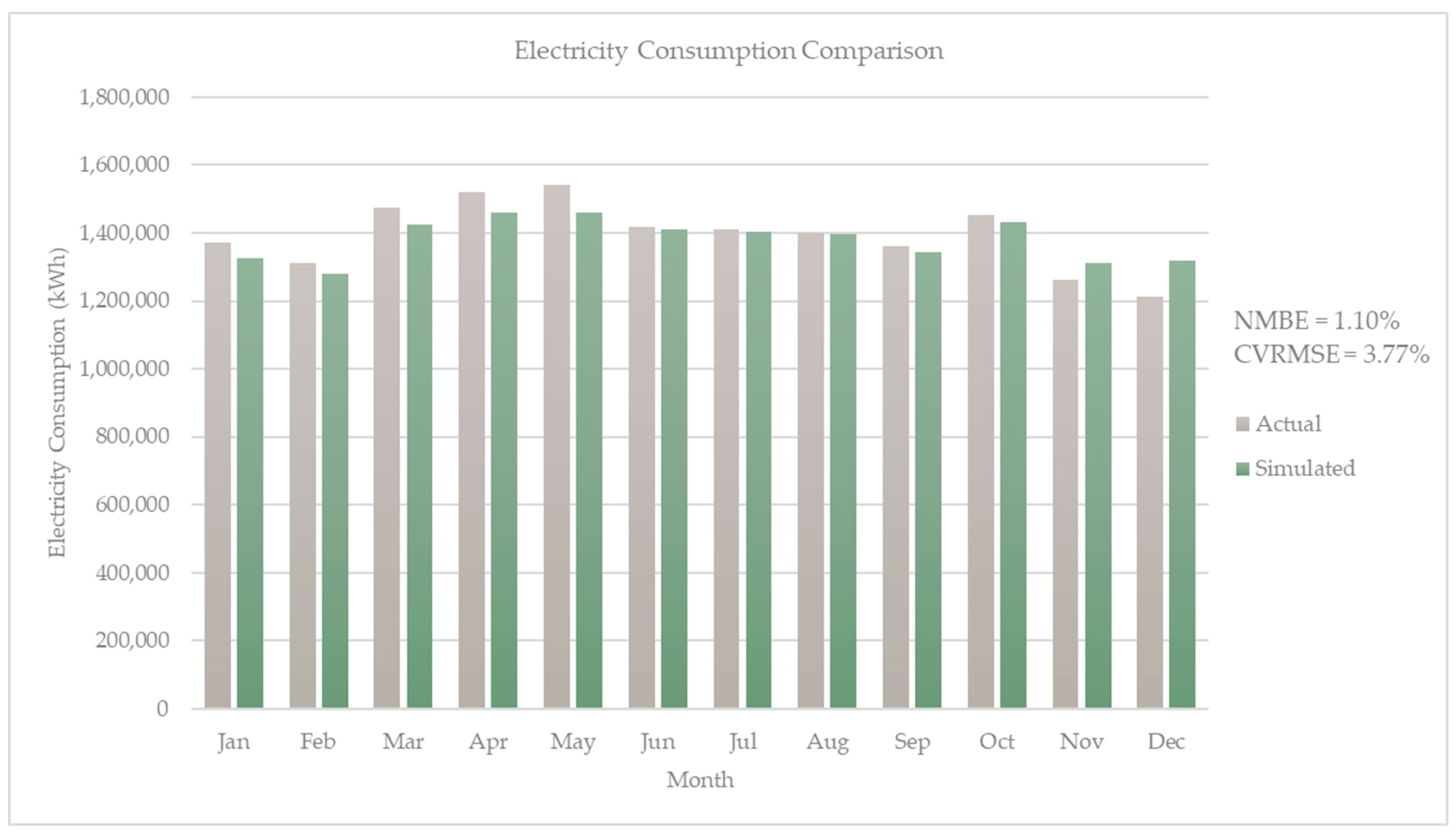
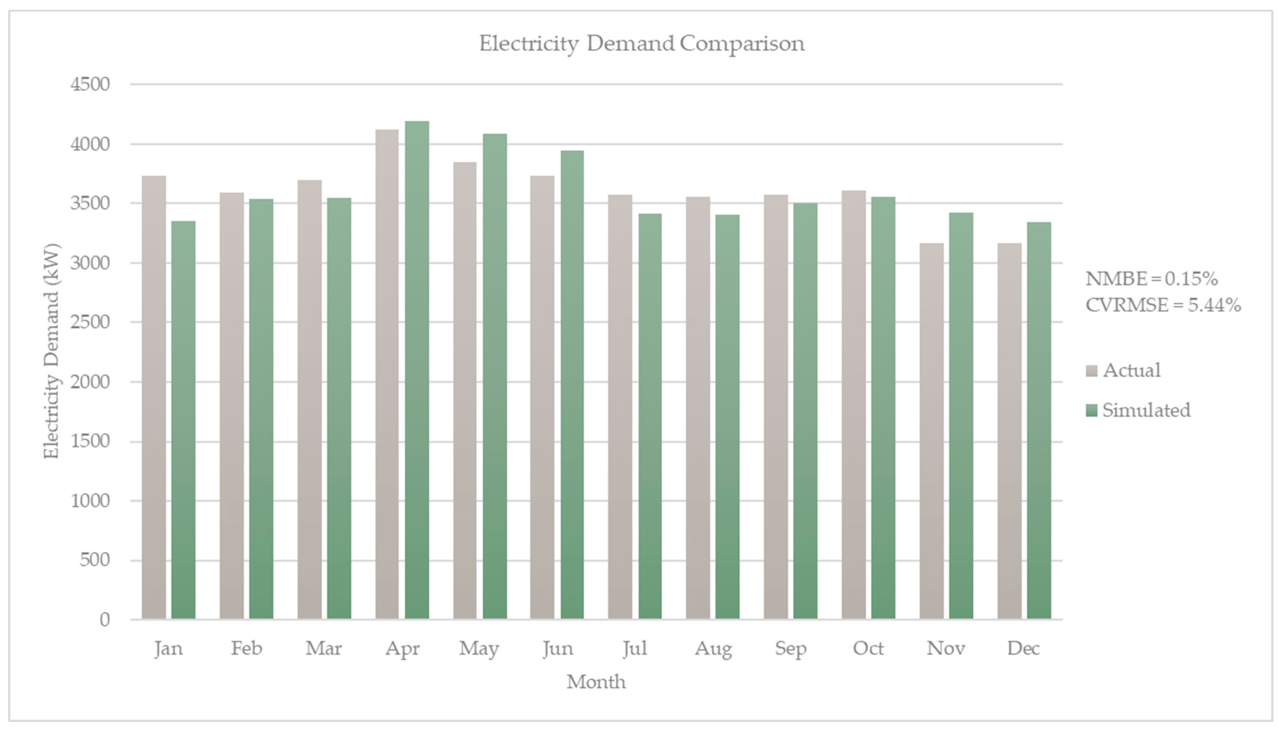
| Month | Electricity Consumption (kWh) | Peak Electricity Demand kW |
|---|---|---|
| January | 1,373,000 | 3736 |
| February | 1,312,000 | 3596 |
| March | 1,473,000 | 3696 |
| April | 1,520,000 | 4123 |
| May | 1,543,000 | 3852 |
| June | 1,418,000 | 3732 |
| July | 1,411,000 | 3572 |
| August | 1,401,000 | 3552 |
| September | 1,362,000 | 3578 |
| October | 1,452,000 | 3608 |
| November | 1,261,000 | 3166 |
| December | 1,213,000 | 3170 |
| Energy Improvement | Reference Model | Proposed Model | Quantity | Life Expectancy |
|---|---|---|---|---|
| Heat protection films | U-5.03 W/sq. m·k | U-4.91 W/sq. m·k | 6306 sq. m | 8 years or more |
| SHGC-0.76 | SHGC-0.56 | |||
| VLT-0.87 | VLT-0.75 | |||
| VSD controls on AHUs | Constant speed | Variable speed | 30 sets | 10 years or more |
| VSD controls on CDWPs and CTs | Constant speed | Variable speed | 20 sets | 10 years or more |
| Water-side system temperature setpoints | Chilled water: | Chilled water: | N/A | N/A |
| 6.67 °C leaving temperature | 8 °C leaving temperature | |||
| 13.33 °C entering temperature | 14 °C entering temperature | |||
| 6.66 °C delta-T | 6 °C delta-T | |||
| Condenser water: | Condenser water: | |||
| 35/28 °C Tdb/Twb | 35/28 °C Tdb/Twb | |||
| 3.7 °C approach | 2.5 °C approach | |||
| 37.8 °C entering temperature | 37.7 °C entering temperature | |||
| 32.2 °C leaving temperature | 30.5 °C leaving temperature | |||
| 5.6 °C range | 7.2 °C range |
| Energy Conservation Measure (ECM) | Description | 1st Year Investment Cost a |
|---|---|---|
| ECM01 | Heat protection films | USD 146,218 |
| ECM02 | VSD controls on AHUs | USD 88,389 |
| ECM03 | VSD controls on CDWPs and CTs | USD 84,251 |
| ECM04 | Water-side system temperature setpoints | USD 0 |
| ECM05 | Water-side system temperature setpoints and heat protection films | USD 146,218 |
| ECM06 | Water-side system temperature setpoints and VSD controls on AHUs | USD 88,389 |
| ECM07 | Water-side system temperature setpoints and VSD controls on CDWPs and CTs | USD 84,251 |
| ECM08 | Water-side system temperature setpoints and VSD controls on AHUs and on CDWPs and CTs | USD 172,640 |
| ECM09 | Water-side system temperature setpoints, heat protection films, and VSD controls on AHUs and on CDWPs and CTs | USD 318,858 |
| Energy Use Data | Acceptance Criteria | Calibration Result |
|---|---|---|
| Monthly electricity consumption, 2019 | −5% < NMBE < 5% | 1.10% |
| CVRMSE < 15% | 3.77% | |
| Monthly electricity demand, 2019 | −5% < NMBE < 5% | 0.15% |
| CVRMSE < 15% | 5.44% | |
| Monthly chiller plant electricity consumption, 2019 | −5% < NMBE < 5% | 3.69% |
| CVRMSE < 15% | 9.81% | |
| Daily chiller plant energy consumption, 2019 | N/A | 4.88% |
| N/A | 13.00% | |
| One month of chiller plant capacities recorded every two hours between 10:00 and 22:00, April 2023 | N/A | 1.92% |
| N/A | 25.05% |
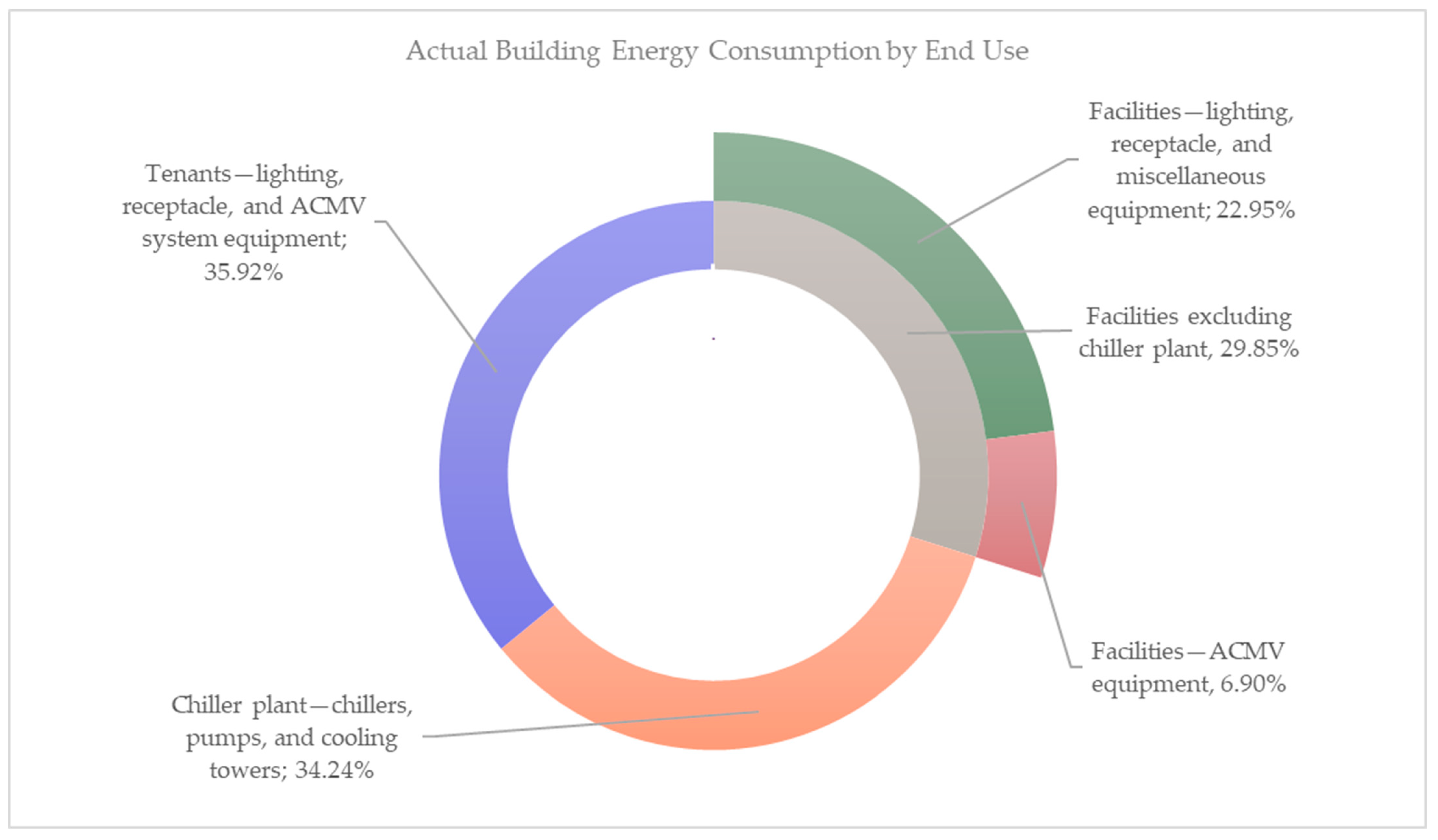
| Energy Conservation Measure, ECM | Energy Consumption (kWh) | Energy Savings (kWh) | EUI (kWh/sq. m) | Operational CO2 Mitigation (tCO2) | Percent Savings |
|---|---|---|---|---|---|
| Reference model | 16,570,497 | - | 275 | - | - |
| ECM01—Heat protection films | 16,391,389 | 179,108 | 272 | 79 | 1.08% |
| ECM02—VSD controls on AHUs | 15,136,128 | 1,434,369 | 251 | 631 | 8.66% |
| ECM03—VSD controls on CDWPs and CTs | 16,413,369 | 157,128 | 273 | 69 | 0.95% |
| ECM04—Water-side system temperature setpoints | 16,166,894 | 403,603 | 269 | 178 | 2.44% |
| ECM05—Water-side system temperature setpoints and heat protection films | 16,001,653 | 568,844 | 266 | 250 | 3.43% |
| ECM06—Water-side system temperature setpoints and VSD controls on AHUs | 14,754,425 | 1,816,072 | 245 | 799 | 10.96% |
| ECM07—Water-side system temperature setpoints and VSD controls on CDWPs and CTs | 16,041,989 | 528,508 | 266 | 233 | 3.19% |
| ECM08—Water-side system temperature setpoints and VSD controls on AHUs and on CDWPs and CTs | 14,607,158 | 1,963,339 | 243 | 864 | 11.85% |
| ECM09—Water-side system temperature setpoints, heat protection films, and VSD controls on AHUs and on CDWPs and CTs | 14,504,147 | 2,066,350 | 241 | 909 | 12.47% |
Disclaimer/Publisher’s Note: The statements, opinions and data contained in all publications are solely those of the individual author(s) and contributor(s) and not of MDPI and/or the editor(s). MDPI and/or the editor(s) disclaim responsibility for any injury to people or property resulting from any ideas, methods, instructions or products referred to in the content. |
© 2024 by the authors. Licensee MDPI, Basel, Switzerland. This article is an open access article distributed under the terms and conditions of the Creative Commons Attribution (CC BY) license (https://creativecommons.org/licenses/by/4.0/).
Share and Cite
Charoenvisal, K.; Sreshthaputra, A.; Pinich, S. Achieving Financial Feasibility and Carbon Emission Reduction: Retrofit of a Bangkok Shopping Mall Using Calibrated Simulation. Buildings 2024, 14, 2512. https://doi.org/10.3390/buildings14082512
Charoenvisal K, Sreshthaputra A, Pinich S. Achieving Financial Feasibility and Carbon Emission Reduction: Retrofit of a Bangkok Shopping Mall Using Calibrated Simulation. Buildings. 2024; 14(8):2512. https://doi.org/10.3390/buildings14082512
Chicago/Turabian StyleCharoenvisal, Kongkun, Atch Sreshthaputra, and Sarin Pinich. 2024. "Achieving Financial Feasibility and Carbon Emission Reduction: Retrofit of a Bangkok Shopping Mall Using Calibrated Simulation" Buildings 14, no. 8: 2512. https://doi.org/10.3390/buildings14082512