Abstract
This article presents the results of a study on the impact of selected parameters of a building’s ground-floor zone (the junction of the external and foundation walls, the ground floor slab, and the ground itself) on the temperature field within the external envelope. This study aims to analyze the influence and optimize the parameters of vertical perimeter insulation in the ground-floor zone of the building. Mathematical modeling was selected as the research method. This paper analyzes the relationships between the temperature ϑimg on the inner surface of the wall at the analyzed node and the linear thermal transmittance coefficient ψim of the thermal bridge occurring in this location, as influenced by the following parameters: dp—thickness of the insulation layer in the ground floor slab; df—thickness of the vertical perimeter insulation layer in the foundation wall; t—location of the insulation layer in the ground floor slab relative to the “external wall-foundation wall” contact surface; r—location of the vertical perimeter insulation layer in the foundation wall; and λs—thermal conductivity of the single-layer external wall material. The analysis was conducted under the climatic conditions of Białystok, Poland. Using THERM 7.6 software for computational experiments, data were obtained to develop deterministic mathematical models of these relationships. The models enabled the assessment of the degree and nature of the influence of the studied factors on ϑimg and ψim, optimization of selected parameters, and mathematical description of safe operating conditions for external walls in the ground-floor zone of heated buildings. It was found that the parameters dp, df, and r have favorable effects, increasing ϑimg by 2.57%, 2.51%, and 4.17%, respectively, when varying from their minimum to maximum levels. Conversely, the parameters t and λs negatively impact ϑimg, contributing reductions of −12.01% and −4.66%, respectively, with a cumulative effect of −16.67%. Optimal parameter values were determined based on energy efficiency criteria. This information may be useful for researchers, designers, engineers, and decision-makers when making informed decisions during the design phase of heated buildings.
1. Introduction
The energy demand for heating buildings in the European Union varies and depends on a number of factors, such as climate, building technologies, energy efficiency standards, and the level of economic development. Buildings have many functions in Europe—residential homes, workplaces, schools, hospitals, libraries, and other public buildings. What they have in common is that they absorb the most energy in the EU. They are also among the largest emitters of carbon dioxide. It is assumed that in European countries, residential buildings are responsible for 40% of energy consumption and 36% of greenhouse gas emissions [1]. These values are largely due to the construction, use, renovation, and demolition of buildings [1,2].
1.1. Thermal Protection Requirements
One of the parameters influencing the heat demand of buildings is the heat transfer coefficient U. In order to compare the level of possible thermal insulation of partitions currently designed, Table 1 presents the current requirements included in Polish regulations [3], requirements for energy-efficient buildings covered by financial support in Poland in 2012–2015 [4], and passive buildings [5].

Table 1.
Maximum values of the heat transfer coefficient U [W/(m2·K)] of the basic building envelope according to different thermal protection standards for heated buildings [3,4,5].
The global energy demand due to heat transfer by penetration through the building envelope takes into account the flow through flat elements of the enclosure, windows, doors, and potential linear thermal bridges (defined in [6]). Recommended maximum values are given in Table 2. In terms of thermal protection of the ground floor, national regulations [3] regarding the connection of a building to the ground require the use of edge insulation in the form of a layer with a thermal resistance of 2.0 (m2∙K)/W around the perimeter of the building.
Table 2.
Recommended values of the linear heat transfer coefficient Ψ [4,5].
In the current technical and construction regulations in Poland, there is no direct limitation regarding the maximum value of the linear heat transfer coefficient Ψ; they were only for buildings supported by the priority program [4]. In the scope of thermal bridges, Polish regulations introduce the requirement of no condensation of water vapor, which enables the development of mold fungi, by checking the value of the temperature coefficient fRsi in the node [3].
Both parameters (Ψ and fRsi) are significantly influenced by the heat transfer coefficient of partition U but also by the shape of the detail, i.e., the mutual position of materials in the construction node. The solution that ensures low values of the linear heat transfer coefficient Ψ and a high value of the temperature coefficient fRsi is the use of a continuous external layer of thermal insulation laid on the outside. There are also single-layer external wall solutions available on the market that meet the requirements for the U coefficient at the level of passive building standards (Table 1 and Table 2). It is a wall made of a single layer of masonry in such a way that in its thickness, there is only one masonry element that performs both a structural and insulating function. Table 3 lists the thermal characteristics of sample products and their dimensions [7,8].
Table 3.
Thermal characteristics of masonry units for single-layer wall construction [7,8].
A special feature of strongly insulated building partitions is that with a decrease in the heat transfer coefficient U of the wall, the risk of increased heat flow through thermal bridges increases [9,10]. Additionally, the risk of thermal bridge intensification may be promoted by the lack of a separate thermal insulation layer in a single-layer wall. Studies show that thermal bridges can be responsible for 30% to 60% of additional heat losses through the building partition [11], which is why they are an important element of the energy balance. The more complex the material arrangement of the joint, the more factors affect the obtained parameters characterizing the thermal bridge. Therefore, designing structural nodes of heated space enclosures is a time-consuming process that often requires multiple revisions of the model geometry (e.g., the thickness of the thermal insulation layer).
1.2. Study of the Variability of Thermal Bridge Parameters
Research on thermal bridges can be divided into those dealing with the theoretical analysis of solutions based on calculations of theoretical models and the results thus obtained. Some researchers undertake in situ testing on sections of actual existing heated buildings. Still, another approach is to test large-scale samples replicating the actual material layout of the envelope conducted in a climate chamber and compare the results with theoretical calculations. A characteristic feature of thermal bridges is their wide variety, which has been somewhat systematized in the standards of reference [12] according to where they occur in the building envelope. However, a single type of bridge can occur in many solution variants and be characterized by extremely different magnitudes of linear heat transfer coefficient Ψ and temperature coefficient fRsi. Small changes in the shape of the detail can significantly affect the above parameters. This is due to publications concerning the special case of a thermal bridge, e.g., comparing the theoretical and actual effects of a reinforced concrete core in a wall corner [13], columns in a frame structure [14,15,16], and a balcony slab [17]. A comprehensive approach to the problem of assessing the sensitivity of various types of thermal bridges classified as in the standard [12] depending on their shape using the NOVA-FAST technique is presented in [18]. The thickness of the inter-story floor slab, the dimension of the reinforcing core in the masonry, the thickness of the masonry in a two-layer wall and the thickness of the masonry in a cavity wall, the thickness of thermal insulation and the heat transmission coefficients of the partitions forming the structural junction were assumed to be significantly influencing the value of the linear heat transfer coefficient. One of the most complicated areas in terms of ensuring thermal insulation continuity is the basement of heated buildings. With floors on the ground, as many as four building elements come into contact in the basement—the external wall, the foundation wall, the floor on the ground, and the soil. More than a dozen materials with very different physical properties form this junction. In addition to the properties of the materials, the mutual location of these materials can have a strong influence on the thermal and moisture processes on the ground floor. One example of a wrong thermal insulation solution in this part of the building and a correct solution is shown in [19]. The amount of heat loss through this part of the building, depending on the heat and moisture flow model used, is shown in [20]. An analysis of the impact of frost insulation variants carried out using CFD techniques is presented in paper [21]. In [22], the authors analyzed the junction of two types of floors on the ground (floors on joists and self-supporting floors) with an external wall made of hemp–lime composite for the occurrence of thermal bridges. Several factors were taken into account that can affect heat transfer at the joint: the level of the floor on the ground, the thickness of the wall, the thermal conductivity of the composite, and the location of the framed structure. Cross-sectionally, the issue of thermal bridging of the building–ground interface was addressed in [23]. The current state of knowledge focusing on the aforementioned detail, the standards used for analysis, the main calculation methods (including dynamic methods), the programming used for analysis, and theoretical and experimental research work are presented. The main part of this work is the case of slab-on-ground with different types of edge insulation, analyzed based on the method of the standard [6] using the THERM program. The large variety of details analyzed in this work has made it possible to conclude that any edge insulation has a high potential for reducing the thermal bridge effect. The issue of this construction node was also addressed in the works [24,25].
After analyzing the above-described studies, it was found that there were no analyses of solutions for single-layer walls. It was considered reasonable to analyze in detail the influence of the five factors selected by the authors on the temperature ϑimg occurring on the surface of the internal wall in the analyzed node and the linear heat transfer coefficient ψim of the thermal bridge occurring in this location. The specificity of thermal bridges is their low repeatability, which requires a detailed thermal analysis of nodes each time, especially in the case of NZEB buildings. The use of knowledge of the dependence of the value of the linear heat transfer coefficient Ψ of a given detail depending on the factors selected by the authors could facilitate and accelerate the design work.
The aim of this study is to analyze the impact and optimize selected parameters of vertical perimeter thermal insulation in the ground-floor zone of a heated building. The analysis is based on mathematical models developed for the temperature dependence ϑimg on the inner surface of the wall and the linear thermal transmittance of the thermal bridge ψim.
The scope of this study will include estimating the degree and nature of the influence of these parameters on selected functions, performing parameter optimization procedures based on an energy criterion, and developing a mathematical description of the safe operating conditions for external walls in the ground-floor zone of heated buildings.
The research presented in this article consisted of the following steps. For the selected five factors influencing the temperature ϑimg and the coefficient ψim, the variability levels were determined. The next stage involved deterministic mathematical modeling based on a symmetric three-level experimental design, using simulation results obtained with the THERM 7.6 software as the foundation. Following the analysis of the influence of the selected factors, their optimization was performed using numerical methods in the MATLAB environment.
The analyzed construction node was examined in terms of temperature, humidity, and energy performance. Furthermore, the optimal solution for this node was identified. The findings of this study expand knowledge about the behavior of similar nodes in buildings, provide valuable guidance on selecting element parameters during their design, and identify safe operating conditions for external walls in the ground-floor zone of heated buildings. The acquired knowledge can be beneficial for researchers, designers, engineers, and decision-makers in making informed decisions during the design phase of heated buildings.
2. Description of the Research Object
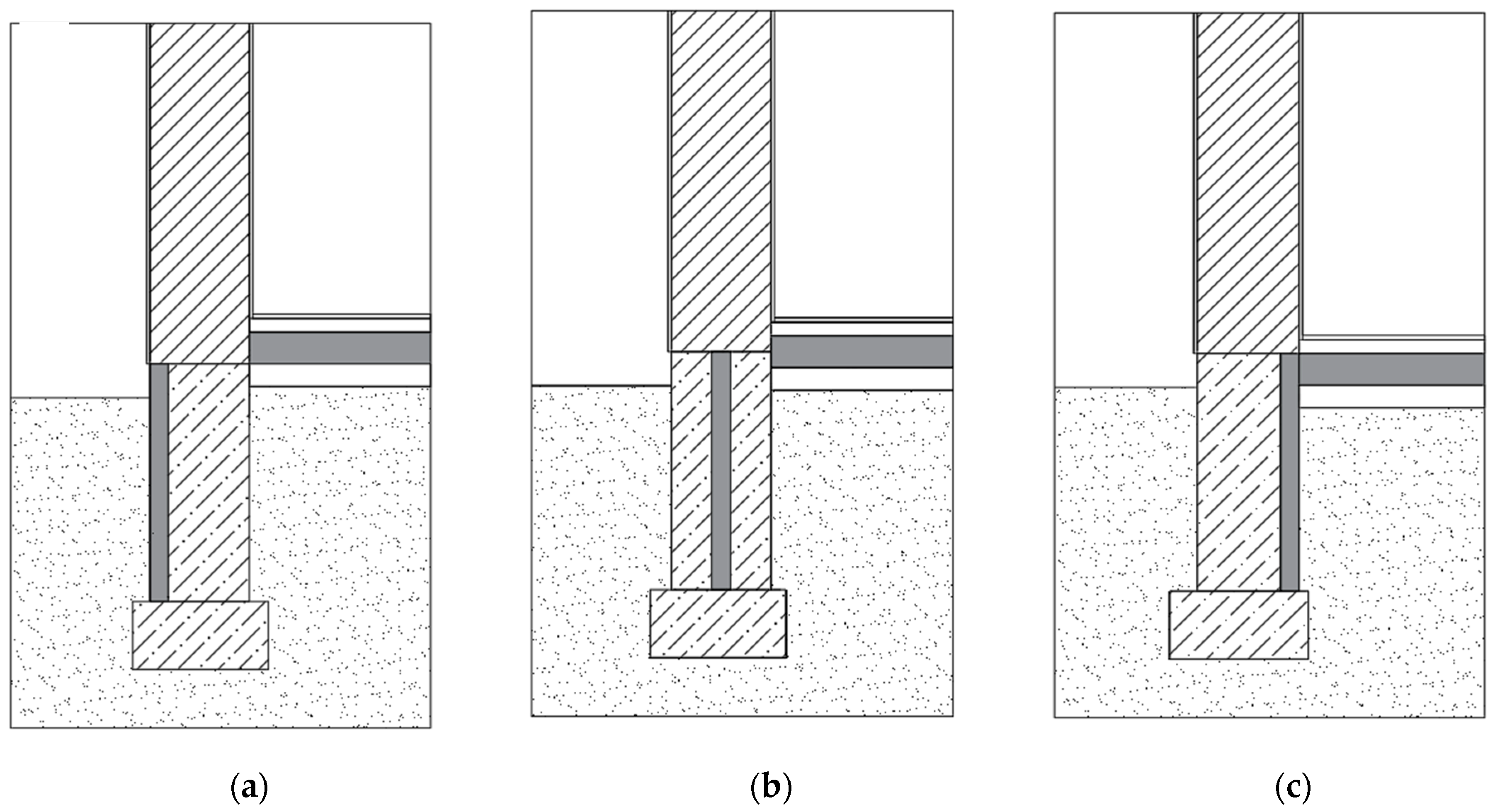
The research was carried out for the connection junction between the floor on the ground and the external wall found on the foundation wall. The solutions adopted are shown in Figure 1, while the material solution is shown in Table 4. The external wall is a single-layer wall of expanded clay with λ = 0.077, λ = 0.095, and λ = 0.113 [W/(m∙K)]. A reinforced concrete two-ply foundation wall with thermal insulation in the form of polystyrene foam with λ = 0.040 [W/(m∙K)] was positioned externally, internally, or in the middle, depending on the design variant. The thickness of the thermal insulation of the foundation wall was assumed to be 4, 6, or 8 cm, depending on the calculation variants. The floor on the ground is laid on a 10 cm thick concrete leveling layer, on top of which a layer of polystyrene thermal insulation is laid with a thickness of 6, 10, or 14 cm, depending on the calculation variant, with a thermal conductivity coefficient of λ = 0.040 [W/(m∙K)]. The effect of the position of the thermal insulation of the floor on the ground in relation to the contact with the foundation wall (top, bottom, center) was also taken into account.
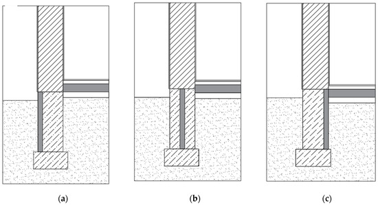
Figure 1.
Solution of selected variants of the analyzed connection junction “external wall-foundation wall-floor” with the location of the thermal insulation layer in the foundation wall ((a) from the external side; (b) in the middle; (c) from the internal side) and in the floor on the ground with regard to the contact surface of the wall with the foundation ((a) upper; (b) in the middle; (c) from below).
Table 4.
Layout and design parameters of the foundation–wall–floor junction.
For the analysis of the problem in this article, the value of B = 8 m. Depending on the purpose of the calculation, 0.5B’/2.5B’ is taken. For the calculation of temperature values, 0.5B’ is taken for the calculation of the Ψ linear heat loss coefficient 2.5B [26].
3. Procedure for Determining the Temperature Fields Within the Thermal Bridge Formation
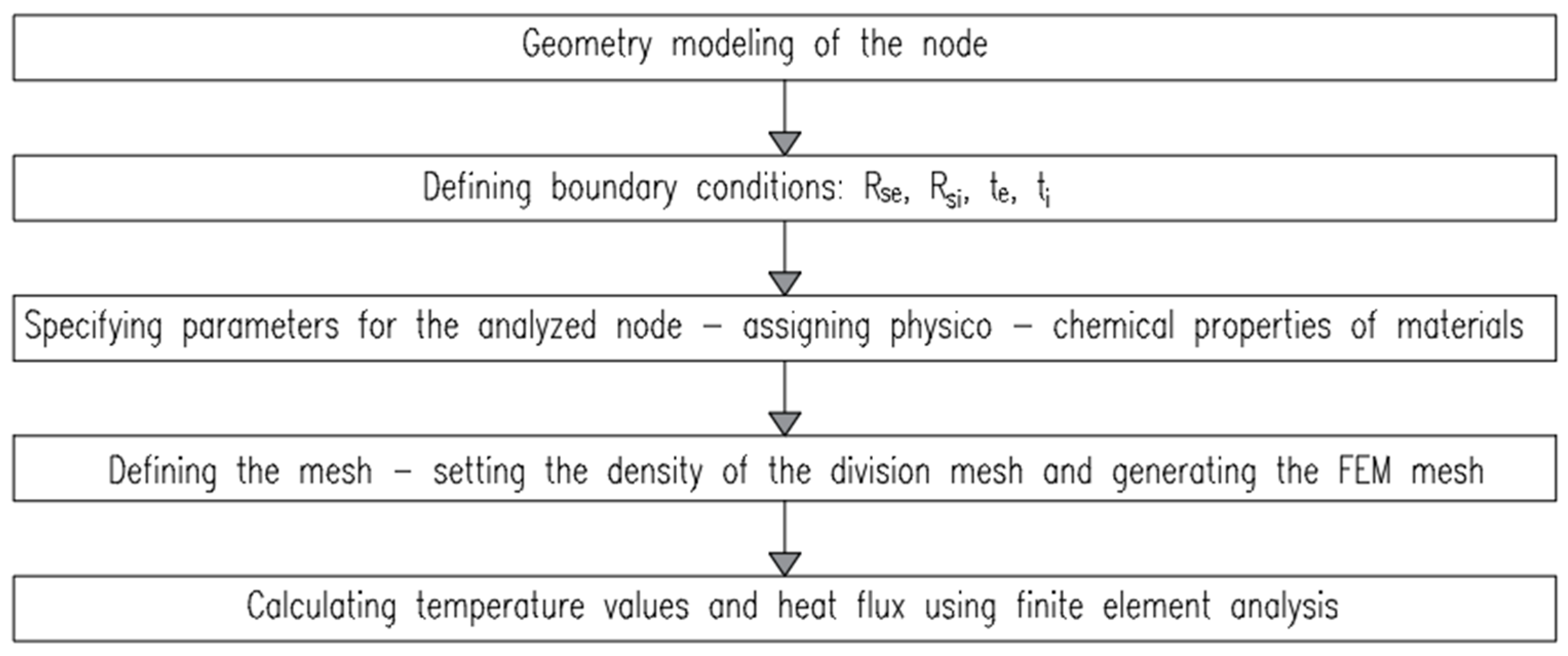
For the calculations of the junction between the external wall and the ground floor slab, the THERM 7.6 software was used. This program employs two-dimensional heat transfer analysis (2D) based on the finite element method (FEM). This method allows for the division of complex geometric elements. After defining the cross-sectional geometry, THERM automatically generates a cross-sectional mesh, performs heat transfer analysis, and runs an error estimation tool. If necessary, it refines the mesh automatically and provides corrected calculations. The program allows one to draw a cross-section either by tracing an imported DXF or bitmap file or by creating the geometry based on a dimensioned drawing. Below is a flowchart used during the calculations performed in the THERM software (Figure 2) [27]:
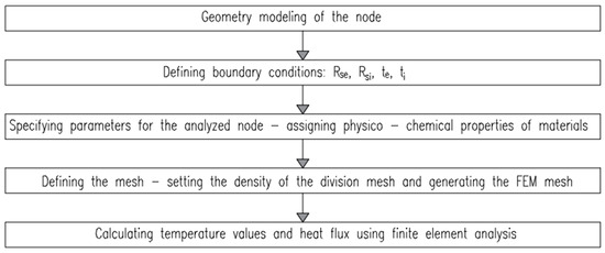
Figure 2.
Flowchart used during the calculations performed in the THERM software.
After proper modeling, the following values can be obtained from the program: the heat transfer coefficient U [W/m2K], the distribution of isotherms, heat flux vectors, and temperature fields.
The modeling conditions of the analyzed details and the boundary conditions were adopted according to the PN-EN ISO 10211 standard [28]:
- -
- For the external surface of the wall, the external air temperature te = −22 °C and Rse = 0.04 [m2·K/W];
- -
- For the external surface of the ground, the outdoor air temperature te = −22 °C and Rse = 0.04 [m2·K/W];
- -
- For internal wall surface, the indoor air temperature ti = 20 °C and Rsi = 0.13 [m2·K/W];
- -
- For the floor on the ground inside the building from above, the indoor air temperature ti = 20 °C and Rsi = 0.17 [m2·K/W].
4. Method of Determining the Temperature Fields Within the Thermal Bridge Formed and the Linear Heat Transfer Coefficient
From the general energy equation [29], the equation determining two-dimensional heat conduction (1) is derived:
where denotes internal heat generation, which corresponds to the following boundary conditions:
—adiabatic boundary condition; —temperature boundary condition; —calculated heat flux boundary condition; —linearized radiation boundary condition; and —radiation boundary condition.
The program for the boundary conditions assumes the surfaces to be grey and isothermal, so α = ε. The H-radiation equation has the form of Equation (2):
where B denotes the surface radius, which is calculated using Equation (3):
In the next step, the program uses the cross rule to calculate the coefficients of view F (4):
Then, using Fourier’s law, the magnitude of the heat flux up to the limit (5) is determined:
The finite element method used in THERM is based on the weighted residuals method, which is based on Equation (6):
When interpreting the results obtained from THERM, it must be taken into account that they are approximate results. The models made in the program are not created from real components. However, the calculation results are within 10% accuracy [29].
The next step is to calculate the linear heat transfer coefficient based on the standard in [27] using Equation (7):
where denotes the thermal coupling coefficient; denotes the heat transfer coefficient of the external wall component above ground ; denotes the minimum distance from the cross-sectional plane connection ; denotes the height of the upper surface of the floor slab above ground level [m]; denotes the heat transfer coefficient of the floor, calculated on the basis of the standard in [30]; and denotes the characteristic dimension of the floor.
In order to accurately calculate , the presence of horizontal and vertical edge insulation should be taken into account. In the analyzed case, there is vertical edge insulation. Therefore, the additional impact of the mentioned insulation must also be taken into account. In such a case, the equation has the following form (8):
Conversely, is calculated from the following formula (9):
where λ denotes the thermal conductivity coefficient of vertical insulation, D denotes the width of vertical edge insulation [m], d’ denotes the additional equivalent thickness calculated from Formula (10), and denotes the total equivalent thickness [m]
where R′ denotes the additional thermal resistance introduced by the edge insulation, and λ denotes the thermal conductivity coefficient of the edge insulation material
where denotes the full wall thickness, including all insulation [m]; denotes the ground thermal conductivity coefficient; denotes the floor thermal resistance, including all insulation layers over the entire surface /W]; denotes the internal surface thermal resistance /W]; and denotes the external surface thermal resistance /W].
5. Mathematical Modeling of the Temperature Dependence at the Thermal Bridge Location and the Linear Heat Transfer Coefficient
A number of principles are recommended when using mathematical modeling. Mathematical models should be brief and use the most important factors describing the characteristics under study. The objective function should be unambiguous, making clear physical sense; quantitatively measurable; not specified as a percentage; informative; and statistically efficient. Factors, on the other hand, should be mutually independent, controllable, non-contradictory, measurable, unambiguous, directly influential, and one order more accurate than the function.
In accordance with the objective of this study, the temperature ϑimg, [°C] at the location of the lowest temperature at the node under study (function Y1) and the linear heat transfer coefficient ψim, [W/(m∙K)] of the thermal bridge occurring at this location (function Y2) were taken as objective functions. It was decided to investigate the influence of five factors on these functions, namely: dp—the thickness of the thermal insulation layer in the floor on the ground (factor X1); df—the thickness of the vertical perimeter thermal insulation layer in the foundation wall (factor X2); t—the location of the thermal insulation layer in the floor on the ground in relation to the “external wall-foundation wall” contact surface (factor X3); r—the location of the vertical perimeter thermal insulation layer in the foundation wall in relation to its internal-external surface (factor X4); and λs—the thermal conductivity coefficient of the material of the single-layer above-ground wall (factor X5).
Natural factors , , and were assumed to be quantitative. In contrast, the factors and are qualitative and vary in increments of +1. With this assumption in mind, the levels of variability of the factors were selected, and in order to ensure the reliability of this study, these were adopted according to the description of the connection node. The levels of variability are recorded below in natural form and in brackets in coded form.
Factor X1 (dp)—the thickness of the thermal insulation layer in the floor on the ground was assumed to be 0.06 (−1), 0.10 (0), and 0.14 (+1) [m]. Factor X2 (df)—the thickness of the vertical perimeter thermal insulation layer in the foundation wall was assumed to be 0.04 (−1), 0.06 (0), and 0.08 (+1) [m]. Factor X3 (t)—location of the thermal insulation layer in the floor on the ground in relation to the “external wall-foundation wall” contact area: upwards-1 (−1), in the middle-2 (0), and downwards-3 (+1) [-]. Factor X4 (r)—the location of the vertical perimeter thermal insulation layer in the foundation wall in relation to its internal-external surface: upwards-1 (−1), inwards-2 (0), and downwards-3 (+1) [-]. Factor X5 (λs)—the thermal conductivity coefficient of the single-layer external wall material is assumed to be 0.077 (−1), 0.095 (0), and 0.113 (+1) [W/(m∙K)]. The values of the factor levels are given in Table 5.
Table 5.
Ranges of variation of the factors X1, X2, … X5 affecting the temperature ϑimg (Y1) of the internal surface of the external wall and the linear heat transfer coefficient ψim(Y2) at the junction “external wall-foundation wall-floor on the ground”.
The transition from the natural values of the factors , , , , and to the corresponding normalized values of X1, X2, X3, X4, and X5 was performed according to Equation (12) [31]:
where , , and are the current, maximum, and minimum natural values of the i-th factor, respectively.
The other input data required for the simulation calculations of the selected objective functions were assumed constant in this study.
It was assumed that the relationships sought Y1,2 = f (X1,X2,X3,X4,X5) could be described by a polynomial of second degree [32]:
Y = a0 + a1 X1 + a2 X2 + a3 X3 + a4 X4 + a5 X5 + a12 X1 X2 + a13 X1 X3 + a14 X1 X4 + a15 X1 X5 + a23 X2 X3+ a24 X2 X4 + a25 X2 X5 + a34 X3 X4 + a35 X3 X5 + a45 X4 X5 + a11 X12 + a22 X22 + a33 X32 + a44 X42 + a55 X52
To obtain a database for modeling and describing the relationships sought, a five-factor computational experiment was carried out according to the optimal second-stage experiment plan (Table 6). Sufficient information about the object in such a situation can be provided by a limited number of data points. For plan selection in this experiment, five five-factor plans were analyzed. A three-level plan was selected for 27 trials with a high D-criterion value of e(D) = 0.972 [33].
Table 6.
Plan of computational experiment for five variables Xi for N = 27 trials and results of simulation calculations of the values of the objective functions Y1 and Y2 ( values in brackets were calculated according to the developed models).
The results of the simulation calculations in the 27 samples analyzed were obtained using the described method with THERM 7.6 software and are presented in Table 6.
Based on the results of calculations using the least squares method [31], deterministic mathematical models were developed in the form of regression equations of the relationship Y1,2, = f(X1,X2,X3,X4,X5):
- -
- The temperature of the inner surface at the thermal bridge ϑimg:
- -
- The linear heat transfer coefficient of the thermal bridge site ψim:
In testing the accuracy, it was taken into account that deterministic models are characterized by a mutually unambiguous correspondence between the external impact and the response to this impact. For this reason, only one experiment was performed at each point in the plan. Testing in this case was carried out using the Fisher criterion, which, in the case of a computational experiment, consists of comparing the mean and residual variance and is calculated according to Equation (16) [31]:
where S2y denotes the variance of the mean, S2r denotes the residual variance, f1 and f2 denote the numbers of degrees of freedom (f1 = (N − 1) = 27 − 1 = 26; f2 = (N − Nb) = 27 − 21 = 6), N denotes the number of calculations performed, and Nb denotes the number of coefficients in the regression equation.
The regression equation describes the results of the calculation adequately if the F value is greater than the tabulated value of Ft at a significance level p and degrees of freedom f1 and f2.
As can be seen from the calculations, F1 = 2.0496/0.1401 = 14.6344 and F2 = 0.0023/0.0001 = 17.9474, while the tabulated value is Ft = F 0.05; 26; 6 = 3.83 [31]. Thus, the F1 and F2 values exceed Ft many times, which means that the models are adequate and useful for further analysis. Their high quality is confirmed by the determination coefficients R2(1) = 0.9879 and R2(2) = 0.9902. The models are original, and it was not possible to compare their accuracy with models existing in the literature. However, we conducted a sensitivity analysis of the obtained models. For this purpose, the values of the studied factors were sequentially changed from 0 to 0.1. It turned out that such fluctuations in the factor values caused changes in the function values; specifically, there were increases in by 0.02 °C (X1, X2) and an increase of 0.033 °C (X4), as well as decreases in by 0.097 °C (for X3) and 0.038 °C (for X5). In this way, we confirmed the high sensitivity of the obtained models.
6. Test Results, Their Interpretation, and Optimization
6.1. Results of This Study
The mathematical models (14) and (15) were used to analyze the effect of the studied factors on the temperature at the thermal bridge location ϑimg (function Y1) together with the linear heat transfer coefficient ψim (function Y2). For better clarity, the discussion of the results was made using natural variables. The word combinations “favourable factor” or “favourable effect” used hereafter mean that with a change in factor from the lower to the upper level, the value of the Y1 function increases, and for the Y2 function, the value decreases.
Analyzing the developed models (14) and (15), the following was detected in the center Gp of the multifactor space, which is characterized by coordinates corresponding to the average level of the factors: the thickness of the polystyrene foam in the floor on the ground, () = 0.10 m; the thickness of the polystyrene foam in the foundation wall, () = 0.06 m; the location of the thermal insulation layer in the floor on the ground, () = 2; the location of the vertical perimeter thermal insulation layer in the foundation wall, () = 2; the thermal conductivity coefficient of the masonry made of expanded clay elements, () = 0.095 W/mK; and the function quantities are temperature ϑimg—function Y1 = 15.82 °C—and linear heat transfer coefficient ψim—function Y2 = 0.142 W/(m2∙K). Then, using the Gp point as a reference point, the degree and nature of the influence of each of the five factors on each of the functions examined were estimated.
6.2. Interpretation
As can be seen from model (14), the factors X1, X2, and X4 show beneficial effects and increase the magnitude of the temperature ϑimg. The effects of their influence when changing from lower to upper levels are, respectively, +2.57, +2.51, and +4.17%. The highest effect was shown by the location of the vertical layer of perimeter thermal insulation in the foundation wall, i.e., factor X4; when increasing from the outer position (1) to the inner position (3), the magnitude of ϑimg increases at 4.17%. The influence of the other two factors, X3 and X5, is related to the reduction of ϑimg. Their contributions were, respectively, −12.01 and −4.66%, and the total contribution of the factors was −16.67%. The most unfavorable contribution is shown by factor X3—the location of the thermal insulation layer in the floor on the ground. When increasing the location of this layer from the top position (1) to the bottom position (3), the magnitude of ϑimg drops to 12 (01%). Thus, it was detected that changing the location of the thermal insulation layers in the considered partitions with their displacement to the inner surfaces (boundaries) of these partitions (level X3 = 1; level X4 = 3) with the remaining factors unchanged can increase the temperature at the thermal bridge location by approximately 2.5 °C (15.82 (4.17 + 12.01)/100 = +2.56 °C).
From model (15), it is detected that factors X1, X2, and X4 also show favorable effects of influence on the linear heat transfer coefficient ψim, lowering it to −13.00, −9.93, and −8.63%, respectively. In contrast, the unfavorable effect associated with increasing the linear heat transfer coefficient ψim is shown by factors X3 and X5 with contributions of +50.39 and +20.80%, respectively. Again, the most unfavorable effect is shown by factor X3—the location of the thermal insulation layer on the floor on the ground; when changing from the top position (1) to the bottom position (3), the magnitude of ψim increases by 50.39%.
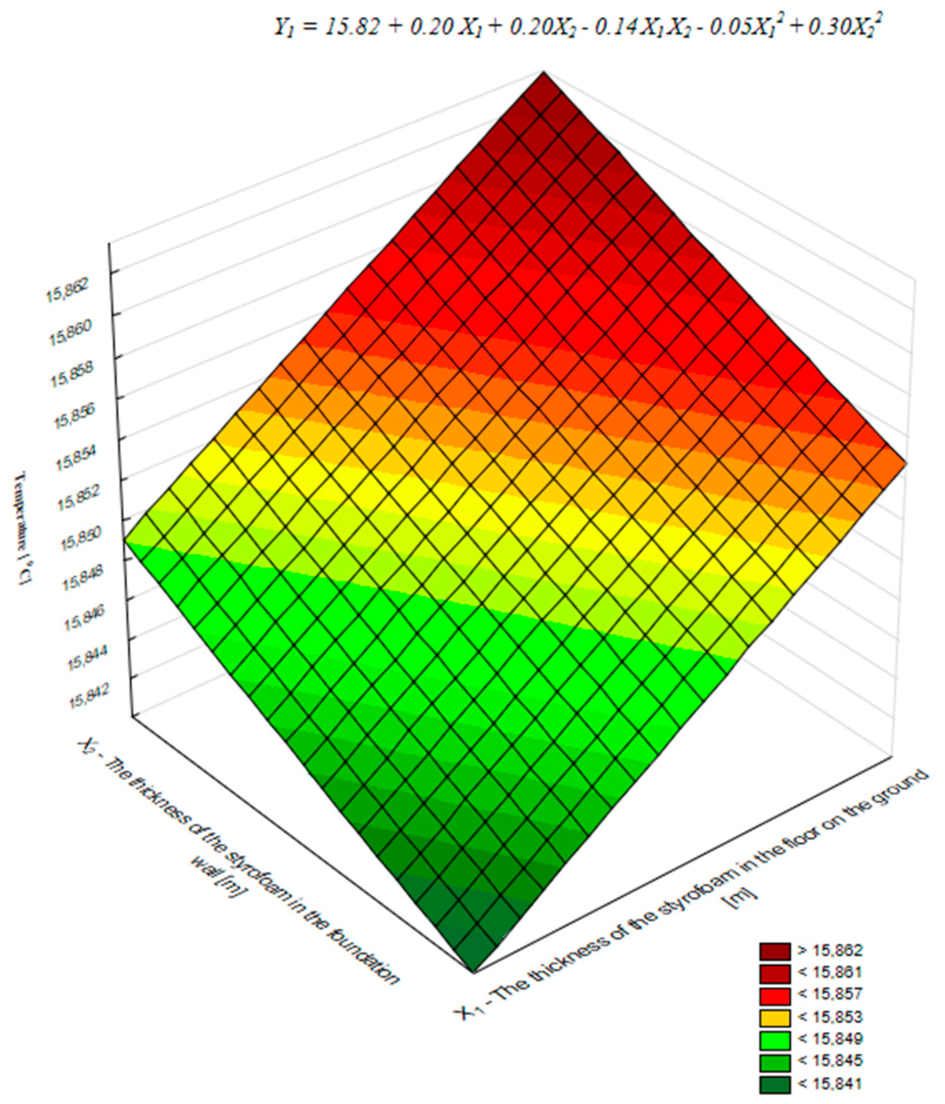
Weak quadratic effects were detected in models (14) and (15). Some coefficients reflect very weak co-factor effects, in addition to the +0.48X3X4 coefficient, which is comparable to the coefficients of linear factor effects −0.97X3 and +0.33X4. Analyzing these coefficients, it can be concluded that the influence of the X3 factor will always be weaker the greater the value of the X4 factor. However, the influence of factor X4 will be stronger the greater the value of factor X3. The nature of the influence of the several factors analyzed is illustrated graphically. Figure 3 shows the dependence of the temperature ϑimg on the following factors: X1—thickness of polystyrene foam in the floor on the ground—and X2—thickness of polystyrene foam in the foundation wall. Figure 4 shows the dependence of the linear heat transfer coefficient ψim on the following factors: X1—thickness of polystyrene foam in the floor on the ground—and X5—heat transfer coefficient of the wall made of porous ceramic elements.
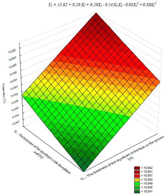
Figure 3.
Temperature dependence of ϑimg on the following factors: X1—thickness of polystyrene in the floor on the ground—and X2—thickness of polystyrene in the foundation wall at X3 = 0, X4 = 0, X5 = 0.
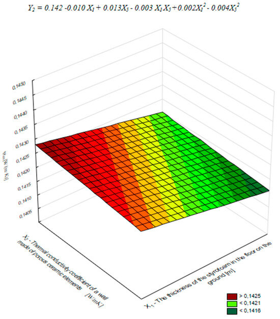
Figure 4.
Dependence of the linear heat transfer coefficient ψim on the following factors: X1—thickness of the polystyrene in the floor on the ground—and X5—thermal conductivity coefficient of a wall made of porous ceramic elements at X2 = 0, X3 = 0, X4 = 0.
6.3. Discussion
The conditions around the tested bridge were then analyzed in terms of temperature, humidity, and energy. The most dangerous effect of thermal bridges is the condensation of moisture due to the reduction of the temperature at the bridge surface below the dew point temperature. A second negative effect is the formation of a relative humidity of 80% and above on the bridge surface, which, according to EN-ISO 13788 [34], can cause mold growth. Therefore, two critical temperature values—the dew point temperature (ts) and the temperature at which a relative humidity of 80% arises on the bridge surface (t80)—had to be determined for the tested linear bridge under the assumed conditions ti = 20 °C and ϕi = 60%. This is determined by two classical relationships:
ϕi = 100 p/ps; ps = f (t)
It turned out that for the assumed air characteristics (ti = 20 °C, ϕi = 60%), ts (cond) = 12.03 °C and t80 (mould) = 15.48 °C occur as critical values in the thermal bridge room. Comparing these values with the results of the calculations at the plan points (Table 6), it can be seen that 9 of the 27 points have ϑimg temperatures with values below 15.48 °C. This means that, for the selected factor values at these points, the level of thermal insulation at the bridging point is insufficient to avoid a relative humidity of 80% and mold growth on the external surface of the linear thermal bridge.
The obtained critical values ts (condensation) and t80 (mold), together with model (14), enabled the authors to create a mathematical description of two safe operating conditions. This represents the most significant practical achievement of the authors in this study. These conditions, presented as mathematical models, allow for a straightforward determination of the operational state of the ground-floor zone—whether it is acceptable or not—for any values of the analyzed factors within their defined variability ranges. The aforementioned conditions are presented below:
1. Condition I operation to prevent condensation on the bridge surface:
15.82 + 0.20X1 + 0.20X2 − 0.97X3 + 0.33X4 − 0.38X5 − 0.14X1 X2 − 0.15X1 X3 + 0.05X1 X4 + 0.09X1 X5 + 0.11X2 X3 + 0.13X2 X4 + 0.13X2 X5 + 0.48X3 X4 − 0.01X3 X5 + 0.08X4 X5 − 0.05X12 + 0.30X22 − 0.64X32 + 0.33X42 + 0.10X52 > 12.03 °C
2. Operating condition II to prevent relative humidity of 80% on the bridge surface (mold growth):
15.82 + 0.20X1 + 0.20X2 − 0.97X3 + 0.33X4 − 0.38X5 − 0.14X1 X2 − 0.15X1 X3 + 0.05X1 X4 + 0.09X1 X5 + 0.11X2 X3 + 0.13X2 X4 + 0.13X2 X5 + 0.48X3 X4 − 0.01X3 X5 + 0.08X4 X5 − 0.05X12 + 0.30X22 − 0.64X32 + 0.33X42 + 0.10X52 > 15.48 °C.
The proposed mathematical descriptions of the operating conditions (18) and (19) make it possible to assess the suitability of numerous combinations of solutions and materials of the elements of the thermal bridge under consideration in terms of temperature and humidity. It should be noted that the fulfillment of condition II always guarantees the fulfillment of condition I but not vice versa.
6.4. Optimization
Optimization of the parameters considered was performed on a mathematical model (15), describing the dependence of the linear heat transfer coefficient ψim on selected parameters. This study initially planned to analyze the ψim coefficient according to the energy criterion. The idea is that when assessing the energy demand of heated buildings, in addition to the heat transfer coefficients of the partitions, we always take into account the linear heat transfer coefficients, which can result in a significant heat loss component in the building. It follows that if thermal bridges cannot be avoided, it is always necessary to reduce their linear heat transfer coefficients ψim to a minimum. The mathematical model developed by the authors (15) is just right for this.
The method used was an iterative (numerical) search of the entire study area, which was adequate with an appropriate sampling step of the individual input factors in the MATLAB environment. The optimization searched for parameter values, ensuring the minimum value of the linear heat transfer coefficient ψim.
It turned out that, despite the complex study area in the form of a five-dimensional factor space, the minimum values of the linear heat transfer coefficient for the node under consideration are at or near the boundary of this area. Three alternative variants of optimum factor values were detected, providing an equal minimum value of ψimmin = 0.078 [W/(m K)] (Table 7).
Table 7.
Optimization results on the mathematical model of the relationship ψim = f (dp, df, t, r, λs).
As can be seen from Table 7, in order to ensure a value of ψimmin = 0.078 [W/(m∙K)], the following should always be used in each of the three variants: thickness of the polystyrene foam in the floor on the ground, dp = 0.14 m; upper location of the thermal insulation layer in the floor on the ground, t = 1; and lowest value of the thermal conductivity coefficient of the wall made of porous ceramic elements of the wall, λs = 0.077 [W/(m∙K)]. The other parameters, df and r, fluctuate. In variant 1, provide both ψimmin at the upper level, namely with the thickness of the polystyrene in the foundation wall (df = 0.08 m), and with the internal location of the vertical perimeter thermal insulation layer in the foundation wall (r = 3). However, in the other variants (2 and 3), the following should be assumed: the values of the thickness of the polystyrene in the foundation wall, which are, respectively, df = 0.06 m and df = 0.04 m, and the location of the vertical layer of perimeter thermal insulation in the foundation wall, which is, respectively, external r = 1 and central r = 0. The calculations show that at the optimum values of the factors (Table 7), the temperature ϑimg on the surface of the tested linear bridge will be about 17.3° C. This temperature value ensures safe operating conditions for the wall in terms of humidity.
After analyzing the influences of the various parameters and optimizing them, the objective of this study was achieved.
7. Conclusions
- This article presents a study on the temperature field in the ground-floor zone elements of a heated building at the contact point “external wall-foundation wall-ground floor slab-ground” under significant variations in internal and external temperatures. The results of this study confirmed the complex nature of the influence of selected parameters and the necessity of performing an optimization procedure. Temperature distribution data were obtained through computational experiments. The calculations were performed using THERM 7.6 software. The obtained data were used to develop deterministic mathematical models of the studied functions. These models enabled the estimation of the degree and nature of the influence of the analyzed factors on the temperature ϑimg and the linear thermal transmittance coefficient ψim. Furthermore, the models allowed for determining the safe operating conditions of the external wall with the above-described solution for the linear thermal bridge in the ground-floor zone;
- From the temperature dependence model ϑimg at the thermal bridge location, it was detected that factors X1, X2, and X4 show favorable effects and increase the magnitude of ϑimg. The effects of their influence when changing from lower to upper levels are, respectively, +2.57, +2.51, and +4.17%. The effects of the other two factors, X3 and X5, are associated with a decrease in ϑimg. Their contributions were, respectively, −12.01 and −4.66%, and the total contribution of the factors to the lowering of ϑimg. was −16.67%. It was also detected that a change in the location of the thermal insulation layers in the considered partitions with a shift to the internal boundaries of these partitions (level X3 = 1; level X4 = 3) with the other factors unchanged could increase the temperature at the thermal bridging site by about 2.5 °C;
- From the dependence model of the ψim coefficient of the analyzed thermal bridge, it was detected that the factors X1, X2, and X4 also show favorable effects of influencing the linear heat transfer coefficient ψim, lowering it to −13.00; −9.93; −8.63%, respectively. On the other hand, unfavorable effects related to increasing the linear heat transfer coefficient ψim are shown by factors X3 and X5 with contributions of +50.39 and +20.80%, respectively;
- On the basis of the temperature dependence model ϑimg at the thermal bridge location, mathematical descriptions were proposed for two conditions for the safe operation of the external wall with the above-described solution of the linear thermal bridge on the ground floor, namely: operation condition I preventing the occurrence of condensation on the bridge surface and operation condition II preventing the occurrence of relative humidity of 80% on the bridge surface (mold development). The mathematical descriptions created make it possible to assess the suitability of the numerous combinations of solutions and materials of the elements of the thermal bridge under consideration in terms of temperature and humidity;
- Based on the model of the relationship for the ψim coefficient of the analyzed thermal bridge, an optimization of the considered parameters was carried out according to an energy efficiency criterion. An iterative search method was applied, exploring the relevant parameter space with an appropriate sampling step for each factor within the MATLAB environment. The optimization aimed to find parameter values that ensure the minimum value of the linear thermal transmittance coefficient ψim. Three alternative sets of optimal parameter values were identified, all providing the same minimum coefficient value of ψimmin = 0.078 [W/(m K)]. The determined optimal parameter values ensure a temperature ϑimg at the thermal bridge location of approximately 17.3 °C, which guarantees safe operational conditions for the wall in terms of moisture protection.
Author Contributions
Conceptualization, W.J., P.S. and C.L.; methodology, W.J., P.S. and C.L.; software, C.L.; validation, W.J.; formal analysis, W.J., C.L. and P.S.; investigation, W.J., C.L. and P.S.; writing—original draft preparation, W.J., P.S. and C.L.; writing—review and editing, C.L., P.S. and W.J.; funding acquisition, C.L., W.J. and P.S. All authors have read and agreed to the published version of the manuscript.
Funding
This research received no external funding.
Data Availability Statement
This study did not report any data.
Conflicts of Interest
The authors declare no conflicts of interest.
References
- European Commission–Department: Energy–In Focus, Energy Efficiency of Buildings Brussels. 17 February 2020, pp. 154–196. Available online: https://commission.europa.eu/news/focus-energy-efficiency-buildings-2020-02-17_pl (accessed on 28 March 2024).
- BPIE—Buildings Performance Institute Europe, Europe’s Buildings Under The Microscope. A Country-by-Country Review of the Energy Performance of Buildings. 2011. Available online: https://bpie.eu/wp-content/uploads/2015/10/HR_EU_B_under_microscope_study.pdf (accessed on 4 December 2016).
- Regulation of the Minister of Develpmant, Work and Technology of 21 December 2020 on Technical Conditions, Which Should Correspond to the Buildings and Their Location. Available online: https://isap.sejm.gov.pl/isap.nsf/DocDetails.xsp?id=WDU20200002351 (accessed on 28 March 2024).
- Priority Program of the National Fund for Environmental Protection and Water Management “Improvement of Energy Efficiency” Part:2: Subsidies to Credits for Construction of Energy-Saving Houses, Years 2012–2015.
- Passivhause Institut. Available online: https://passipedia.org/basics/building_physics_-_basics/what_defines_thermal_bridge_free_design (accessed on 1 April 2024).
- ISO 10211:2017; Thermal Bridges in Building Construction—Heat Flows and Surface Temperatures–Detailed Calculations. ISO: London, UK, 2007.
- Chruściel, W.; Sulik, P. Wytyczne do projektowania konstrukcji murowych w systemie Porotherm Dryfix. 2012, 1, 38–47. Available online: https://www.wienerberger.pl/content/dam/wienerberger/poland/marketing/documents-magazines/brochures/PL_MKT_DOC_POR_wytyczne_do_projektowania_konstrukcji_murowych_w_systemie_porotherm_dry%EF%AC%81x.pdf (accessed on 10 June 2024).
- Technical notebook. In Projektowanie Architektoniczne i Konstrukcyjne Budynków w Systemie Ytong, wyd; Xella Polska sp. z o.o: Warszawa, Poland, 2017.
- Theodosiou, T.G.; Papadopoulos, A.M. The impact of thermal bridges on the energy demand of buildings with double brick wall constructions. Energy Build. 2008, 40, 2083–2089. [Google Scholar] [CrossRef]
- Kim, M.-Y.; Kim, H.-G.; Kim, J.-S.; Hong, G. Investigation of Thermal and Energy Performance of the Thermal Bridge Breaker for Reinforced Concrete Residential Buildings. Energies 2022, 15, 2854. [Google Scholar] [CrossRef]
- Smusz, R.; Korzeniowski, M. Experimental investigation of thermal bridges in building at real conditions, E3S Web Conf. In Proceedings of the 17th International Conference Heat Transfer and Renewable Sources of Energy, Międzyzdroje, Poland, 3 December 2018; Volume 70. [Google Scholar] [CrossRef]
- ISO 14683:2017; Thermal Bridges in Building Construction—Linear Thermal Transmittance—Simplified Methods and Default Values. ISO: London, UK, 2017.
- Evola, G.; Gagliano, A. Experimental and Numerical Assessment of the Thermal Bridging Effect in a Reinforced Concrete Corner Pillar. Buildings 2024, 14, 378. [Google Scholar] [CrossRef]
- Chandrasiri, D.; Gatheeshgar, P.; Ahmadi, H.M.; Simwanda, L. Numerical Study of Thermal Efficiency in Light-Gauge Steel Panels Designed with Varying Insulation Ratios. Buildings 2024, 14, 300. [Google Scholar] [CrossRef]
- Michálková, D.; Ďurica, P. Measured Impact of Material Settlement in a Timber-Frame Wall with Loose Fill Insulation. Buildings 2023, 13, 1622. [Google Scholar] [CrossRef]
- Milovanović, B.; Bagarić, M.; Gaši, M.; Vezilić Strmo, N. Case Study in Modular Lightweight Steel Frame Construction: Thermal Bridges and Energy Performance Assessment. Appl. Sci. 2022, 12, 10551. [Google Scholar] [CrossRef]
- Zhang, X.; Jung, G.-J.; Rhee, K.-N. Performance Evaluation of Thermal Bridge Reduction Method for Balcony in Apartment Buildings. Buildings 2022, 12, 63. [Google Scholar] [CrossRef]
- Capozzoli, A.; Gorrino, A.; Corrado, V. A building thermal bridges sensitivity analysis. Appl. Energy 2013, 107, 229–243. [Google Scholar] [CrossRef]
- Sedlakova, A.; Majdeln, P.; Tazky, L. Energy efficient buildings—lower structure. Tech. J. 2014, 425–432. Available online: https://suw.biblos.pk.edu.pl/downloadResource&mId=1149294 (accessed on 10 June 2024).
- Deru, M. A Model for Ground-Coupled Heat and Moisture Transfer from Buildings. Technical Report; 2003; pp. 66–72. Available online: https://www.nrel.gov/docs/fy01osti/29693.pdf (accessed on 10 June 2024).
- Stolarska, A.; Strzałkowski, J. Modelling of Edge insulation depending on bounduary conditions for the ground level. IOP Conf. Ser. Mater. Sci. Eng. 2017, 245, 042003. [Google Scholar] [CrossRef]
- Brzyski, P.; Grudzińska, M.; Majerek, D. Analysis of the Occurrence of Thermal Bridges in Several Variants of Connections of the Wall and the Ground Floor in Construction Technology with the Use of a Hemp–Lime Composite. Materials 2019, 12, 2392. [Google Scholar] [CrossRef] [PubMed]
- El Saied, A.; Maalouf, C.; Bejat, T. Etienne Wurtz c Slab-on-grade thermal bridges: A thermal behavior and solution review. Energy Build. 2022, 257, 111770. [Google Scholar] [CrossRef]
- Godlewski, T.; Mazur, Ł.; Szlachetka, O.; Witowski, M.; Łukasik, S.; Koda, E. Design of Passive Building Foundations in the Polish Climatic Conditions. Energies 2021, 14, 7855. [Google Scholar] [CrossRef]
- Wesołowska, M.; Hołownia, P. Izolacje termiczne posadzek budynków niepodpiwniczonych ze ścianami jednowarstwowymi. In Proceedings of the VII Ogólnopolska Konferencja Naukowo-Techniczna Energodom 2004, Kraków, Poland, 13 October 2004. [Google Scholar]
- EN ISO 13788:2012; Hygrothermal Performance of Building Components and Building Elements—Internal Surface Temperature to Avoid Critical Surface Humidity and Interstitial Condensation—Calculation Methods. ISO: London, UK, 2012; ISO 13788:2012, Corrected version 2020-05.
- Available online: https://windows.lbl.gov/therm-software-downloads (accessed on 1 January 2024).
- PN-EN ISO 10211-1; Mostki Cieplne w Budynkach. Obliczanie Strumieni Cieplnych i Temperatury Powierzchni. Część 1:Metody ogólne. ISO: London, UK, 2008.
- Finlayson, E.; Mitchell, R.; Arasteh, D.; Windows and Daylighting Group. THERM 2.0: Program Description, A PC Program for Analyzing the Two-Dimensional Heat Transfer Through Building Products; Building Technologies Department Environmental Energy Technologies Division, Lawrence Berkeley National Laboratory: Berkeley, CA, USA, 1998.
- PN-EN ISO 13370:2017; Thermal Performance of Buildings. Heat Transfer via the Ground. Calculation Methods. ISO: London, UK, 2017.
- Brodsky, V.Z. Tables of Experimental Plans for Factor and Polymial Models; Metallurgy: Moscow, Russia, 1982. [Google Scholar]
- Available online: https://www.statsoft.pl/textbook/stathome.html (accessed on 1 January 2024).
- Korzyński, M. Methodology of the Experiment. Planning, Implementation, and Statistical Analysis of the Results of Technological Experiments; WNT: Warsaw, Poland, 2006. [Google Scholar]
- Durakovic, B. Design of Experiments Application, Concepts, Examples: State of the Art. Period. Eng. Nat. Sci. 2017, 5, 421–439. [Google Scholar] [CrossRef]

Disclaimer/Publisher’s Note: The statements, opinions and data contained in all publications are solely those of the individual author(s) and contributor(s) and not of MDPI and/or the editor(s). MDPI and/or the editor(s) disclaim responsibility for any injury to people or property resulting from any ideas, methods, instructions or products referred to in the content. |
© 2025 by the authors. Licensee MDPI, Basel, Switzerland. This article is an open access article distributed under the terms and conditions of the Creative Commons Attribution (CC BY) license (https://creativecommons.org/licenses/by/4.0/).