Spatial Characteristic Analysis of Near-Fault Velocity Pulses Based on Simulation of Earthquake Ground Motion Fields

Abstract

The spatial variation characteristics of near-fault velocity pulses lack in-depth understanding, and it is difficult to consider this feature in probabilistic seismic hazard analysis and the ground motion input for structural seismic analysis. Based on ground motion simulation, this study performs spatial characteristic analysis of velocity pulses. The Mw 6.58 strike-slip Imperial Valley and the Mw 6.8 dip-slip Northridge earthquakes are adopted as the cases, and the simulation method is validated by comparing synthetics with observations. The multi-component broadband ground motion fields are simulated, and the pulse parameters and the pulse area are extracted using the multi-component pulse identification method. The spatial characteristics of various pulse parameters are analyzed. The results show that for a single earthquake, the pulse period is a spatial variable related to source-to-site geometry, the pulse amplification factor has great spatial variation, and the orientation of the maximum pulse component is controlled by the radiation pattern. Finally, the influence of slip distribution on pulse is explored based on two earthquakes, in which the uniform slip, the random slip, and the hybrid slip are combined with different rupture directions. This study contributes to a more reasonable consideration of pulse-like ground motion in seismic risk assessment and earthquake response analysis.

1. Introduction

In 1990s, several major earthquakes (i.e., the 1994 Northridge earthquake in California, the 1994 Kobe earthquake in Japan, and the 1999 Chichi earthquake in Taiwan) caused severe damage to a large number of building structures, and this damage was exacerbated by bidirectional pulses caused by rupture directionality or unidirectional pulses related to surface faulting and static offset. From then on, near-fault pulse-like ground motion has attracted great attention in the field of engineering seismology and earthquake engineering. The long-period components of near-fault velocity pulses have a huge destructive effect on long-period structures, such as high-rise buildings, large-span spatial structures, and long bridges. Reasonably expressing the impact of ground motion pulses in the seismic hazard analysis of engineering structures has become a topic of concern. Some frameworks have been proposed to incorporate the effect of near-fault pulses into probabilistic seismic hazard analysis [1,2,3]. These frameworks have two basic terms; the pulse model that predicts the occurrence probability of pulses [4,5] and the ground motion prediction equation (GMPE) considering the pulse effect [6,7]. These two terms play a fundamental role and have a significant influence on the results of probabilistic seismic hazard analysis.

Accounting for the pulse effect in a GMPE is often realized by combining a base GMPE with a pulse amplification factor [6], in which the base equation predicts the response spectra of ground motion without any pulse, and the pulse amplification factor expresses the amplification of response spectra due to the presence of a pulse. The pulse amplifies the response spectra over a narrowband of periods centered about the pulse period [8,9], and this is often modeled by an amplification factor with a bell-shape functional form [1,10,11,12]. In these fixed functional forms, the pulse period is the only variable and thus it is the key parameter. Currently, most studies model the pulse period as a function of magnitude [1,8,13], and thus the pulse period and the pulse amplification factor are only dependent on magnitude and are independent of source-to-site geometry and source mechanism. The pulse period has clear variations with source-to-site geometry, as found by a previous numerical study [14], but this spatial information is intermixed because the pulse prediction models in probabilistic seismic hazard analysis are developed using near-fault records from many earthquakes with different mechanisms. Thus, the spatial variation characteristics of pulse parameters, including pulse period and pulse amplification factor, need to be inspected.

Additionally, the pulse model that predicts the occurrence probability of pulses is usually developed using the dataset of near-fault strong-motion records, including both pulse-like and non-pulse-like ground motions, from past earthquakes [1,4,13,15]. Most pulse models [1,4,13] are built based on two-dimensional geometrical parameters [16] and thus are applied, respectively, for two rupture types, namely the pure strike-slip rupture and the pure dip-slip rupture. It is not clear which type of model should be used for the oblique-slip earthquake. A three-dimensional geometrical parameter [17] can eliminate the limitations of two-dimensional parameters, and Dadras et al. [15] used it as a predictive variable to develop the pulse model [18]. The pulse occurrence probability model is greatly related to the spatial area that exhibits pulses, and the development of pulse models ignores the influence of nonuniform slip distribution. As expected from research on long-period ground motion, slip distribution would greatly affect the spatial area and features of near-fault velocity pulses. Thus, it is necessary to analyze the basic characteristics of the relationship between slip distribution and the pulse area.

As the strong-motion records in a single earthquake are very sparse, it is hard to analyze the spatial variation of pulses based on the seismic observation data empirically. Some studies [19,20,21] use the numerical simulation method to investigate the pulse features of strong-motion records. Referring to this idea, we further promote the use of simulated ground motion fields as the database of spatial analysis.

This study aims to investigate the spatial variation characteristics of near-fault velocity pulses based on ground motion simulation. The 1979 Mw 6.58 strike-slip Imperial Valley earthquake and the 1994 Mw 6.8 dip-slip Northridge earthquake in California are taken as the cases to examine the pulse variation for two types of earthquake mechanisms, and the reliability of the simulation method is analyzed based on the strong-motion records. Then, the multi-component broadband ground motion fields are generated, and the pulse parameters, including the pulse period, the pulse amplification factor, and the orientation of the maximum component are identified to analyze their spatial variation. Finally, based on the two earthquakes, the influence of slip distribution on pulse area and pulse period is investigated, and its implication on the future improvement of the pulse prediction model is proposed.

2. Ground Motion Simulation Method

The finite-fault source model is widely adopted for various methods of ground motion simulation. In this study, the broadband ground motion of the ijth subsource is simulated using a frequency–wavenumber approach (FK) that convolves the Green’s function with the kinematic rupture process [22], as given by

$$a_{ij}(t)=G_{ij}(t)\ast STF({\tau }_{ij},t)M_{0ij}$$

(1)

in which G_ij is the Green’s function from the ijth subsource to the ground point; STF is the source time function that has the same form for all subsources [23]; and τ_ij is the rise time of the ijth subsource. The source time function and the rise time are combined to describe the moment release rate of each subsource in this method. The subsource motions are superposed with time delay, as expressed by

$$a(t)={\displaystyle \sum _{i=1}^{N_L}{\displaystyle \sum _{j=1}^{N_W}{a}_{ij}}(t-\Delta t_{ij}^{\prime }-\Delta t_{ij}^{″})}$$

(2)

in which N_L and N_W are the numbers of subsources along the strike and down dip, respectively; $\Delta t_{ij}^{\prime }$ is the rupture time of the ijth subsource; and $\Delta t_{ij}^{″}$ is the propagation time of seismic wave from the ijth subsource to the offshore site. The Green’s function is calculated using a frequency–wavenumber algorithm [24], following previous studies [19,20].

The simulation method considers two kinds of randomness in the rupture process. The first one is achieved by the incorporation of high-wavenumber random slip into the spatial distribution of slip on the rupture plane [22,25], as described in Equation (6). The second one is expressed by the frequency-dependent radiation pattern model [26], which uses the frequency dependence of the strike, dip, and rake for each subsource to describe the roughness of the rupture plane and the variability in the slip direction. In the calculation of the Green’s function, the time step is 0.02 s and the Nyquist Frequency is 25 Hz. These ensure that the maximum frequency of the obtained ground motion can reach 20 Hz. Further details of the simulation method can be found in our previous study [22].

The FK approach can express the influence of crustal structure on wave propagation and generate ground motions in the fault-normal (FN) and fault-parallel (FP) directions. These features are important to reveal the spatial characteristics of long-period ground motion pulses. Additionally, this study requires broadband simulation rather than long-period simulation because the ratio of energy in the long-period pulse to that in the broadband motion is the primary indicator to judge if the ground motion is pulse-like [13,27]. Based on previous studies [19,20], the FK approach is suitable for simulating the ground motion field for the spatial characteristic analysis of near-fault pulses. Note that the simulation method is based on the layered crustal model and does not consider the local soil-site condition, and thus caution should be exercised when applying these simulation methods in regions with rapid changes in the crustal structure and the near-surface soil layer.

3. Simulation of Ground Motion Fields and Pulse Identification

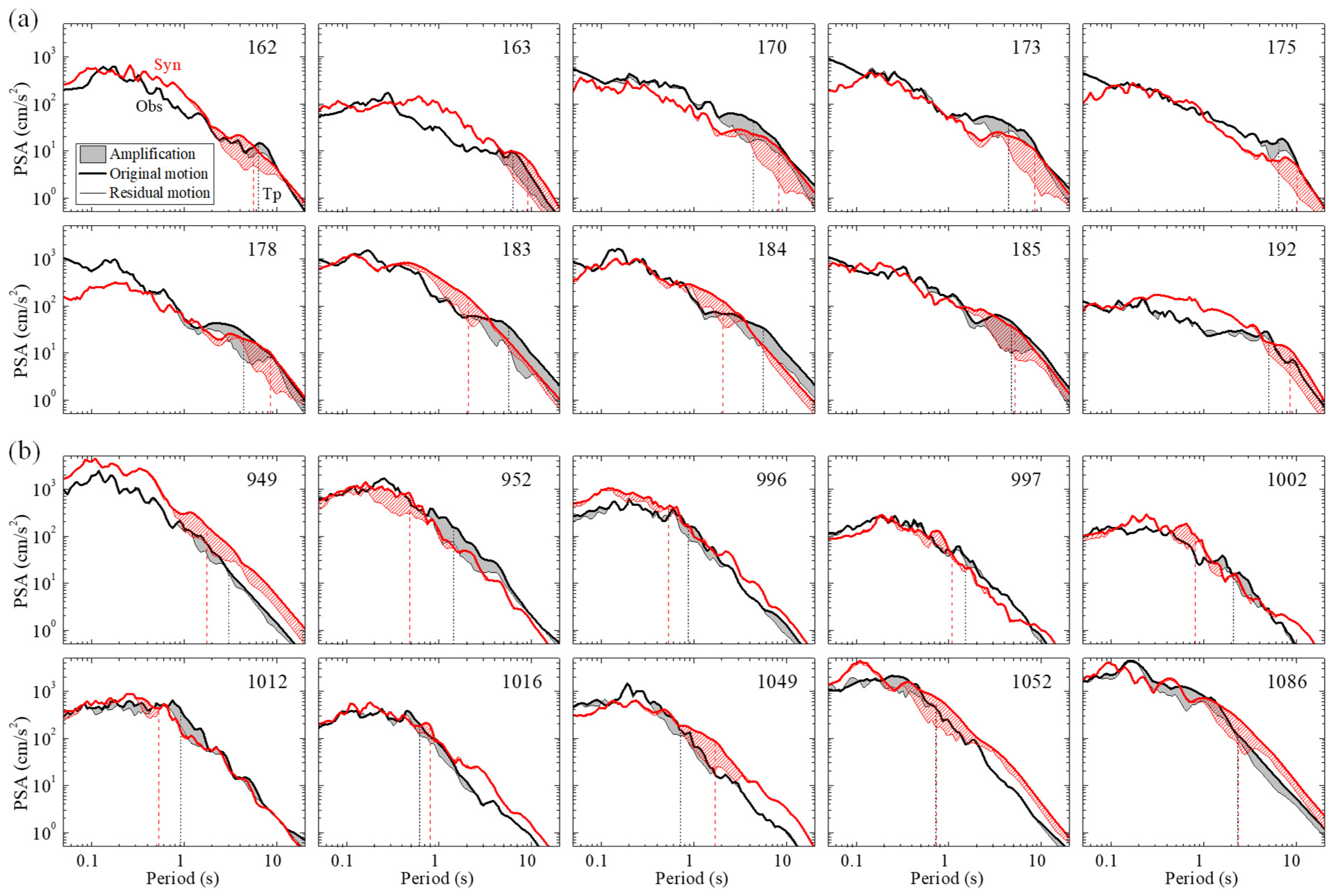
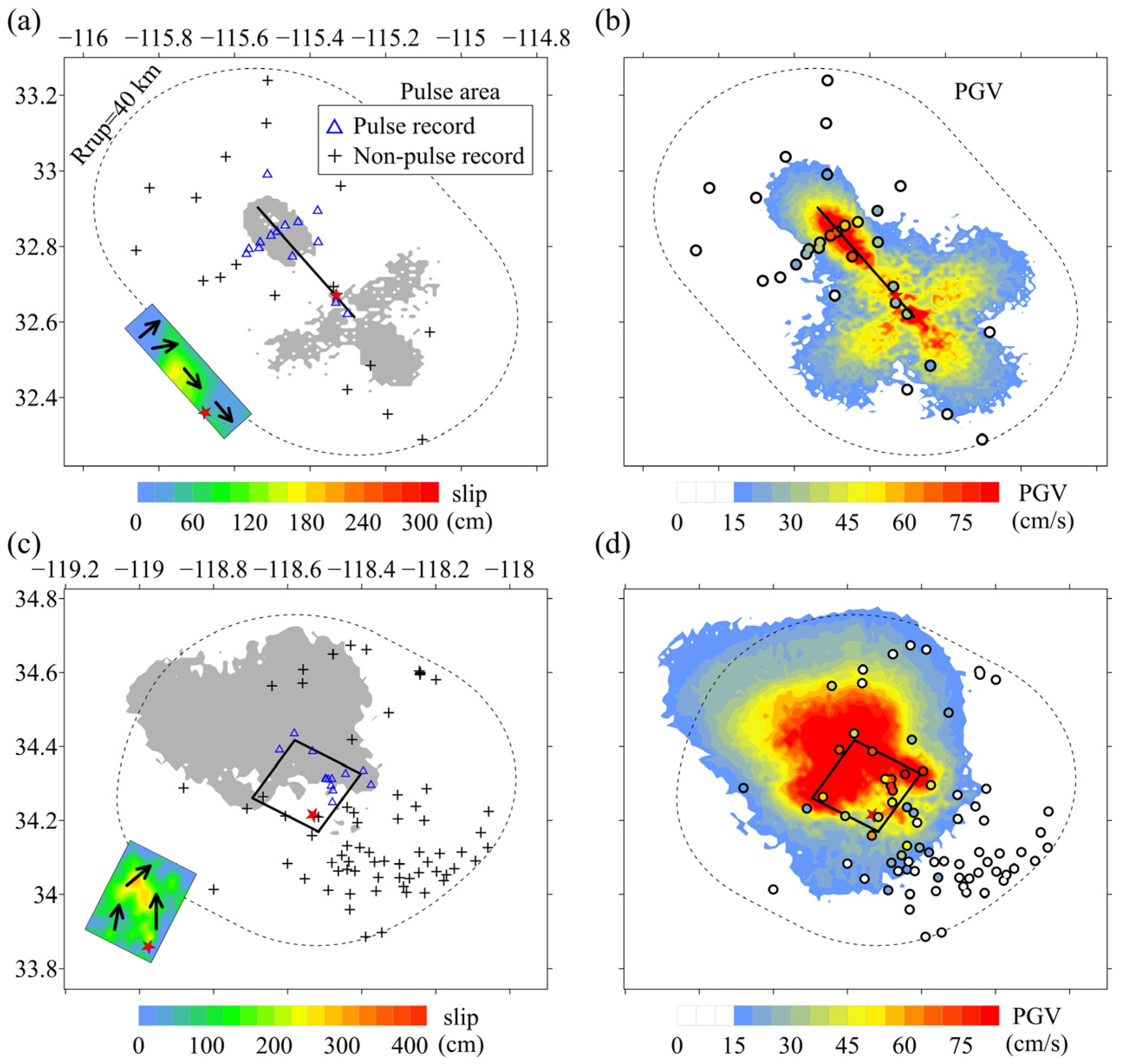
3.1. Simulation of Ground Motion Fields

The 1979 Mw 6.58 strike-slip Imperial Valley earthquake and the 1994 Mw 6.8 dip-slip Northridge earthquake, which have the most pulse-like records in California, are selected as the cases of this study. This section firstly analyzes the efficiency of the FK approach by comparing the synthetics with the observations for the two earthquakes. In the simulation, the moment magnitude, strike, dip, and distributions of slip and rake on the fault plane are adopted from Hartzell and Heaton [28] for the Imperial Valley earthquake and from Wald et al. [29] for the Northridge earthquake. The determination of source parameters has also taken into account relevant studies in recent years [30,31,32]. For the two earthquakes, the energy magnitude used for source constraint is estimated based on McGarr and Fletcher [33]. The energy magnitude is adopted as a complement to the moment magnitude to constraint the rupture process, following our previous study [22]. The generic rock velocity structure is from Graves and Pitarka [34], in which a representative 1D velocity profile is constructed by averaging the profiles sampled at each of the strong-motion recording sites and also constraining V_S30 (the time-averaged shear-wave velocity to a depth of 30 m, a key index to account for site condition) to be 865 m/s. Considering that the large pulse mainly occurs in the near-fault region, the strong-motion records at stations within a rupture distance of 40 km are adopted.

Table 1. Parameters used in the ground motion simulation of the two earthquakes.

Parameters	Imperial Valley	Northridge
Moment magnitude	6.58	6.8
Energy magnitude	6.6	6.7
Source mechanism	Strike-slip	Dip-slip
Strike	323°	122°
Dip	90°	40°
Average rake	180°	101°
Fault depth	0 km	5 km
Fault length and width	42 km × 10.4 km	18 km × 24 km
Number of subsources	16 × 8	16 × 16
Stress drop	2.5 MPa	6 MPa
Velocity structure	[34]	[34]
Slip and rake distributions	[28]	[29]
Number of records	31	83
Number of pulse-like records	14	13

summarizes the various parameters used in the simulation. Further details of stations and corresponding records can be found in the NGA-West2 database [35] by the record sequence numbers. The NGA-West2 database includes worldwide ground motion data recorded from shallow crustal earthquakes in active tectonic regimes and a set of small-to-moderate-magnitude earthquakes in California. Ground motions and metadata for earthquake source, propagation path, and site conditions are provided.

Then, the rock-site (V_S30 of 865 m/s) broadband ground motions (0.1–20 Hz) at all the stations are simulated for the two earthquakes and then compared with the observed records. For consistency, the observed ground motion measures at the strong-motion stations with varying V_S30 are corrected from varying local site conditions to generic rock-site conditions using the site-response factors of the GMPE of Boore et al. [36]. For quantitative evaluation, we calculate the observed-to-synthetic bias [34,37] of the 5% damped pseudospectral acceleration (PSA), peak ground acceleration (PGA), and peak ground velocity (PGV). The pseudospectral acceleration is for the horizontal RotD50 component [38], and the peak values are the geometric average of those of two horizontal components. The residual between the observed and synthetic motions is calculated at each station, and the model bias is the average of residuals over all stations. A perfect match between the observations and the synthetics would have a bias value of 0, and a positive value would indicate underestimation. Figure 1a,c show the bias values of pseudospectral acceleration and peak values, and Figure 1b,d compare the observed and synthetic PGV with the rock-site estimates from the GMPE. The bias values close to zero and the small deviations in Figure 1 indicate that the simulation method provides a good estimation of peak values and pseudospectral acceleration at the entire period range for the two earthquakes. The observed and synthetic PGV values are in good agreement at different distances, and their attenuations with distance closely follow the trend of the GMPE.

Based on the wavelet analysis, Baker [27] proposed a pulse identification method to extract the strongest pulse from the FN component and then to identify the pulse-like ground motion. Shahi and Baker [13] extended the method of Baker [27] to the multi-component pulse identification (in brief, SB14), in which bihorizontal ground motions are rotated to different orientations and the strongest pulse is extracted for identification. In the following studies, the results of the multi-component pulse identification provide the data foundation of pulse models [1,13,15], and thus we use the SB14 method to determine pulse characteristics. In this study, the component from which the strongest pulse is extracted is taken as the analysis object and denoted as the maximum component.

Figure 2 compares the observed and synthetic PSA of the maximum component at 10 stations for each earthquake. In the figure, the residual ground motion is computed by extracting the strongest pulse from the original motion, and the difference between the two kinds of PSA is the amplification of PSA due to the presence of the pulse. For the Imperial Valley earthquake, the synthetic PSA accords well with the observed PSA at six stations (162, 173, 175, 183, 184, 185), has larger amplitude at two stations (163, 192), and has smaller values at two stations (170, 178). For the Northridge earthquake, the observed and synthetic PSA accord well at most stations, especially for 997, 1002, and 1012. The pulse characteristics including pulse amplification and pulse period for the synthetic motions have close performance to those of the observed motions. This indicates that the pulse characteristics of observations can be reproduced by the FK approach.

Figure 3 compares the observed and synthetic velocity time histories of the maximum component at six stations for the Northridge earthquake. At these stations, the shape and amplitude of velocity pulse of the synthetics accord well with those of the observed motions. This result suggests that the FK approach can produce large pulses. Using the simulation models and parameters in Table 1, the pulse periods of the synthetics are similar to those of the observations. Additionally, the pulse period has clear variation among different stations, and this feature is expressed in the synthetic motions. We can conclude from Figure 3 that the ground motion fields simulated using the FK approach have the potential to express the spatial variation of near-fault velocity pulses.

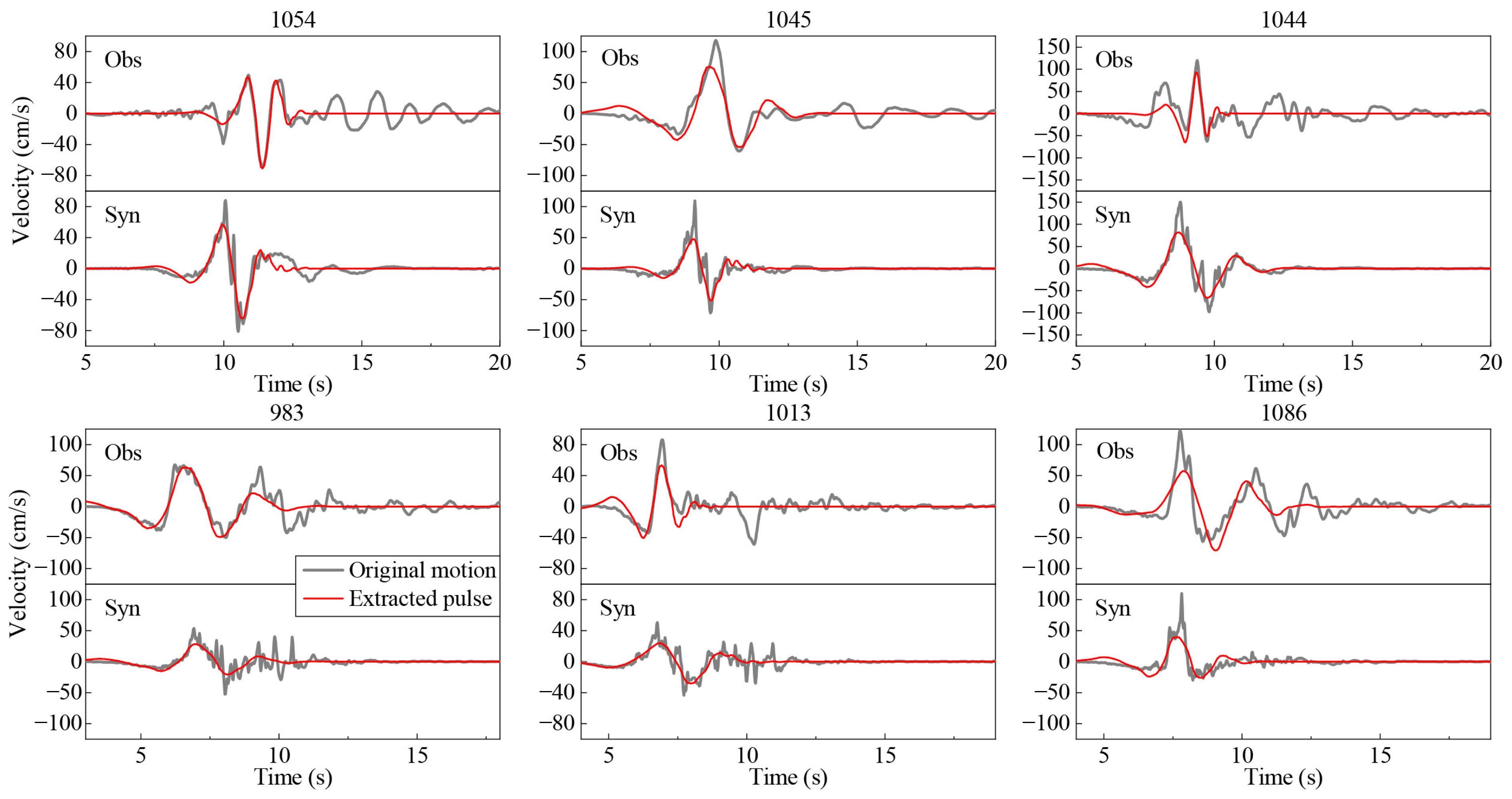
3.2. Pulse Identification of Ground Motion Fields

The above validation suggests that the FK approach can effectively simulate the near-fault ground motions for the two earthquakes. Then, the calculation area with a size of 120 km × 120 km is set around the center of fault projection, and 14,641 ground points are evenly distributed with intervals of 1 km along north and east. The ground motion fields are simulated for the two earthquakes, and the pulse period, pulse amplification factor, and orientation of the maximum component are determined for all ground points, no matter whether the ground motion is pulse-like. This can fully express the spatial variation of pulse characteristics.

Figure 4 plots the pulse area identified by SB14 and the PGV distribution of the synthetic ground motion field for the two earthquakes. The figure also shows the pulse identification results and the PGV of the observed records and the slip distribution. The Imperial Valley and Northridge earthquakes have some common conditions that are favorable for generating pulses; for example, the hypocenter at the bottom right corner of the fault is conducive to the strong propagation effect along the strike and up dip, and the asperity near the center of the fault maximizes the propagation effect. Figure 4 indicates that the PGV distribution of the synthetic field shows good agreement with that of the near-fault observations, and the pulse area accords with the distribution of pulse-like and non-pulse-like records. The pulse area of the synthetic field is larger than the observations in past earthquakes. The main reason is that the randomness of the rupture process is not considered in the simulation and this greatly increases the coherency of long-period ground motions from subsources. For the Imperial Valley earthquake, the pulse area near the epicenter is because the pure strike-slip rupture is conducive to the generation of pulses in the FP motion.

4. Spatial Characteristic Analysis of Near-Fault Pulses

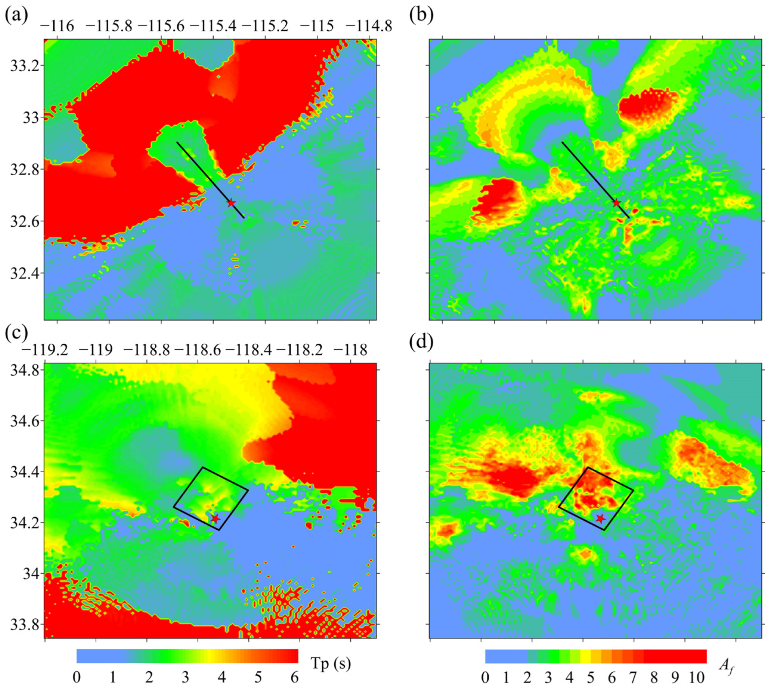
4.1. Spatial Analysis of the Pulse Period and Amplification Factor

Accounting for the pulse effect in a GMPE is realized by combining the base GMPE with the pulse amplification factor [6]. The method can be represented by

$$\ln S{a}_{\mathrm{pulse}}(T,M,R,\xi )=\ln Sa(T,M,R)+I_{\mathrm{pulse}}(M,R,\xi )\ln A_f(T,T_P)$$

(3)

where $\xi$ is the three-dimensional geometrical parameter that describes the rupture propagation effect; $Sa(T,M,R)$ is the PSA of period $T$ at distance $R$ from an earthquake with magnitude $M$; $I_{\mathrm{pulse}}$ is an indicator that has a value of 1 if the ground motion contains a pulse and 0 otherwise; and $A_f(T,T_P)$ represents the amplification of $Sa$ due to the presence of a pulse. $I_{\mathrm{pulse}}$ is related to the pulse model $P(\mathrm{pulse}|M,R,\xi )$ that estimates the occurrence probability of pulses according to magnitude, distance, and source-to-site geometry.

The pulse amplification factor $A_f(T,T_P)$ amplifies $Sa$ at periods close to the pulse period $T_P$, and it can be calculated by Equation [1]

$$A_f(T,T_P)=S{a}_{\mathrm{origin}}/S{a}_{\mathrm{residual}}$$

(4)

where $S{a}_{\mathrm{origin}}$ and $S{a}_{\mathrm{residual}}$ denote the PSA of the original and the residual ground motions, respectively. $A_f(T,T_P)$ is modeled by a function of the normalized pulse period $T/T_P$ [6], and $T_P$ is estimated from the relationship with magnitude [1,13,16]. In the present models, the magnitude-dependent $T_P$ is the only variable in $A_f$. This means that for an earthquake with a given magnitude, $T_P$ and $A_f$ are independent of source-to-site geometry and rupture type.

Figure 5 shows the spatial distributions of $T_P$ and $A_f(T=T_P)$ for the two earthquakes. It is evident from Figure 5a,c that $T_P$ is not a constant but a spatial variable related with source-to-site geometry. The spatial distribution of $T_P$ for the dip-slip earthquake is more complex than that for the strike-slip earthquake due to the combined contribution of the propagation effect and the rupture effect. Figure 5b,d suggest that $A_f(T=T_P)$ also has great spatial variation, and this is related to the fault geometry. Thus, the long-period pulse has some deterministic characteristics, and these should be considered in the pulse prediction models.

4.2. Spatial Analysis of Orientation of the Maximum Pulse Component

Pulse-like ground motions can be observed in many orientations besides the FN component, and sometimes the FN component is not in the orientation that exhibits pulse (e.g., Howard et al. [39]). This phenomenon also appears in the synthetic ground motion field. To simplify the analysis, we take $\alpha$ as the angle between the orientations of the maximum pulse component and the FN component, and set $\beta$ as the half of the orientation range that exhibits pulse, as illustrated in Figure 6. The ranges of $\alpha$ and $\beta$ are $[0°,90°]$, and when $\beta <\alpha$, the pulse cannot be observed in the FN component.

The ground motion pulse usually has a period longer than 0.6 s [40] and the long-period ground motion is deterministic. According to the studies on strong-motion records of past earthquakes [41,42,43,44], the observed radiation pattern readily follows the theoretical one of a double-couple source at low frequencies (<1 Hz), and varies randomly at high frequencies due to the complexity of the source rupture and the small-scale heterogeneity of crust. The radiation pattern can reflect the source-to-site azimuthal effect on the ground motion. As the slip distribution of a moderate–strong earthquake is nonuniform along the strike and down dip, it is difficult to obtain the theoretical radiation pattern. Following Takenaka et al. [41], the radiation pattern is determined approximately by the equation

$$R_{\mathrm{FN}}(f)={\displaystyle \frac{A_{\mathrm{FN}}^2(f)}{A_{\mathrm{FN}}^2(f)+A_{\mathrm{FP}}^2(f)}}$$

(5)

where $A_{\mathrm{FN}}(f)$ and $A_{\mathrm{FP}}(f)$ are the Fourier amplitudes of the FN and FP components, respectively. Generally, $R_{\mathrm{FN}}(f<0.5 \mathrm{Hz})$ is quite close to the theoretical pattern. This study adopts $R_{\mathrm{FN}}(0.3 \mathrm{Hz})$ because most pulse periods are between 3 and 4 s.

Figure 7 shows the spatial distributions of $\alpha$, $\beta$, and $R_{\mathrm{FN}}(0.3 \mathrm{Hz})$ for the two earthquakes. The radiation pattern that is controlled by the dip and rake angles of the seismic source determines the orientation of the maximum component. A previous study [45] has a similar result in that the maximum component often occurs in the orientation with the maximum PGV value. As expected, the radiation pattern is large along the slip direction and becomes small to zero along the normal of slip direction. The nonuniform slip distribution and the fault geometry cause the distortion of the radiation pattern, but four lobes of the theoretical pattern still exist. For the strike-slip earthquake, the FN component is much larger than the FP component in the majority of the pulse area, and thus the maximum component is quite close to the FN component, whereas for the dip-slip earthquake, the FN component is larger than the FP component in a small part of the pulse area. Figure 7c,f also indicate that $\beta$ in the majority of the pulse area is smaller than 45° for the strike-slip earthquake and larger than 45° for the dip-slip earthquake. For the Northridge earthquake, $\beta$ above the upper left corner of the fault is close to 90°, indicating that the pulse can be observed at any orientation.

4.3. Relationship Between $A_f$, $\alpha$, and $\beta$

Parameter $\alpha$ reflects the relative intensity of the FN component to the FP component, and $A_f$ expresses the relative intensity of the original motion to the residual motion. Previous studies show that $A_f$ is stable concerning the change of $\alpha$ [1], and this result is obtained based on empirical analysis of strong-motion records. However, the spare records in a single earthquake cannot express the variation of $A_f$ with $\alpha$ in the ground motion field. Figure 5 and Figure 7 suggest that the distributions of both $A_f$ and $\alpha$ have clear spatial changes. Here, we discuss the variation of $A_f$ with $\alpha$ in the synthetic ground motion field. The pulse amplification factor for each ground point is calculated by Equation (4) and then averaged for different ranges of $\alpha$. Figure 8 shows the variation of $A_f$ with $\alpha$, along with the $A_f$ models in previous studies [1,10,11]. The calculated $A_f$ is quite close to the previous models in the strike-slip Imperial Valley earthquake and for small $\alpha$ in the dip-slip Northridge earthquake. A remarkable feature in Figure 8 is that the calculated $A_f$ is significant for the large $\alpha$ in the Northridge earthquake. The possible reason is that a large pulse occurs at the rupture end of the Northridge earthquake.

Additionally, the variation of $A_f$ with $\alpha$ is also investigated based on pulse-like ground motion records. A previous study by Dadras et al. [15] built a dataset from the NGA-West2 database, which compiles 802 observed records within a rupture distance of 30 km from 64 earthquakes with magnitudes from 5.6 to 7.9. Dadras et al. [15] identified 134 pulse-like records caused by the rupture directivity effect. This study performs pulse identification for all 802 records and finds 175 pulse-like records, including both directivity and nondirectivity pulses. All the directivity and nondirectivity pulses are pooled together for analysis. Similar to Figure 8, Figure 9 shows the pulse amplification factor in different ranges of $\alpha$ for 175 pulse-like records. As the records from earthquakes with different mechanisms are used together, $A_f$ has small differences for different ranges of $\alpha$. The pulse amplification factor of the observed records is close to previous models, and their difference at long periods is because the records in this study are within a rupture distance of 30 km. At a large distance, the residual motions have a significant long-period component, so that the pulse amplification factor is relatively small. With the accumulation of pulse-like records, this obviously discrete feature requires inspection for the improvement of the future empirical model.

For the 175 pulse-like records, Figure 10 shows the distribution of $\beta$ with $\alpha$ for different source mechanisms. Most pulses are observed in the $\alpha$ range $[0^{°},{30}^{°})$, especially for strike-slip earthquakes. For the dip-slip and oblique-slip earthquakes, a larger proportion of pulse-like records cannot be observed in the FN component. In addition, $\beta$ is larger than 30° for most records, indicating that the pulse can be observed in a wide range of orientations.

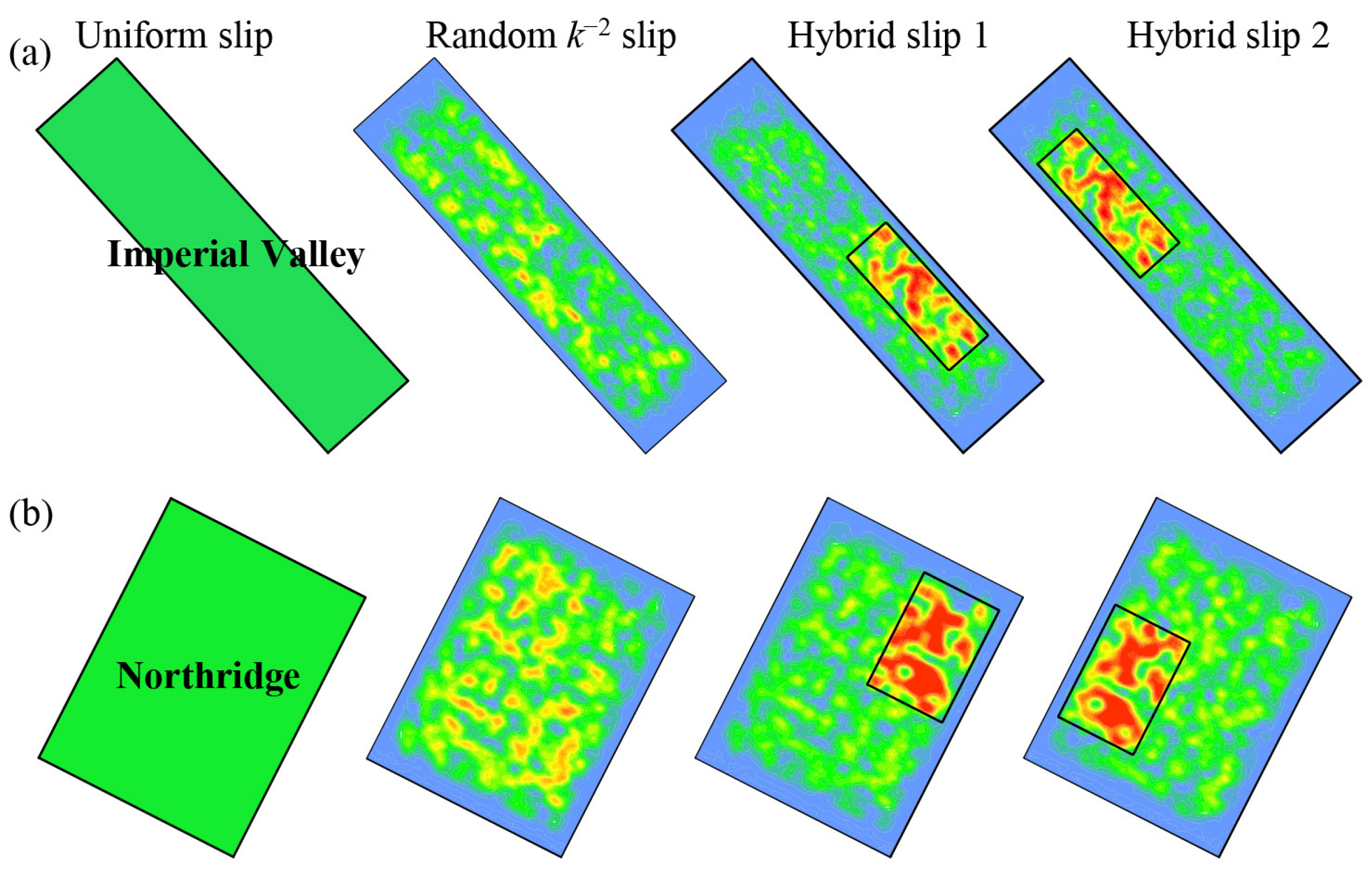
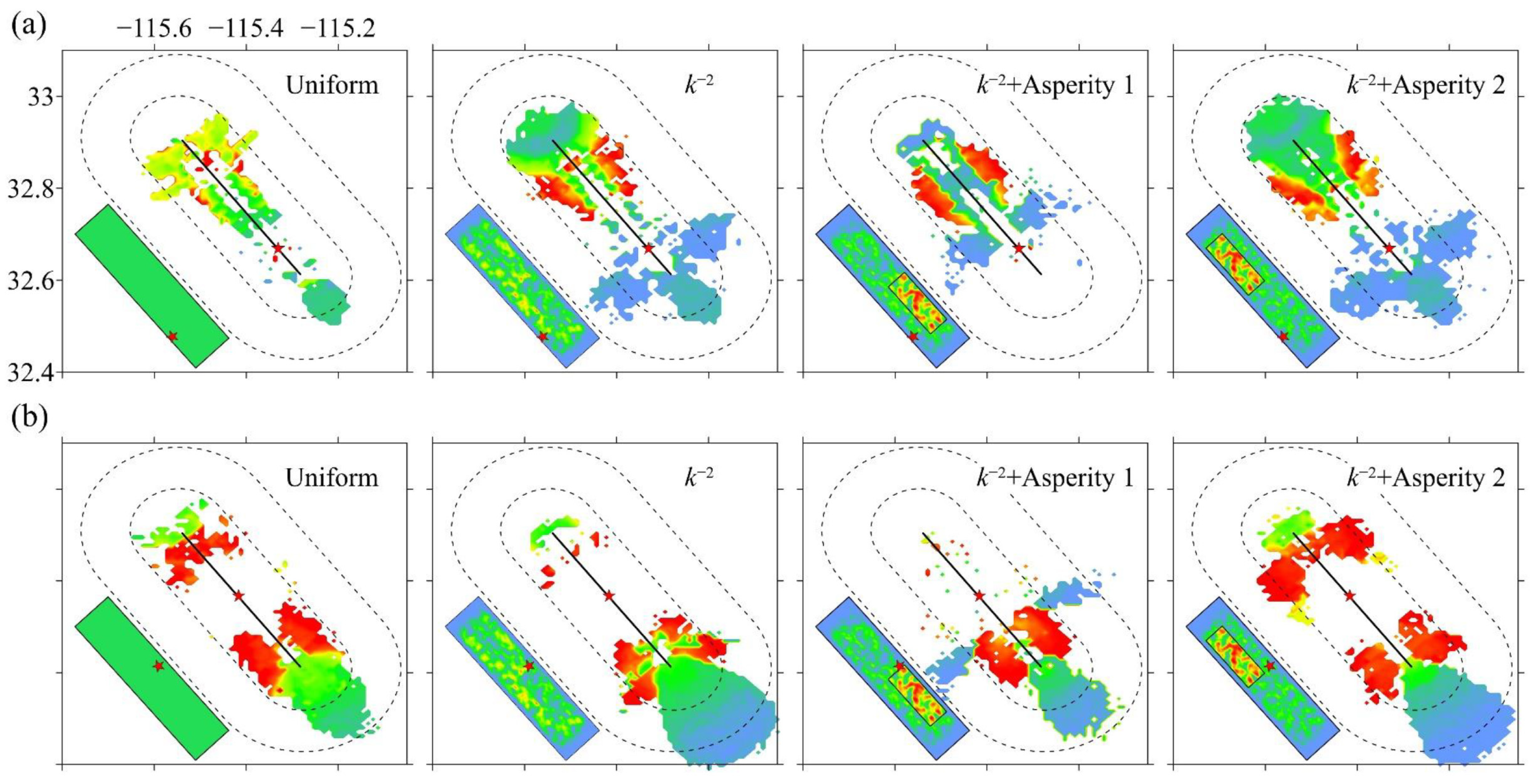
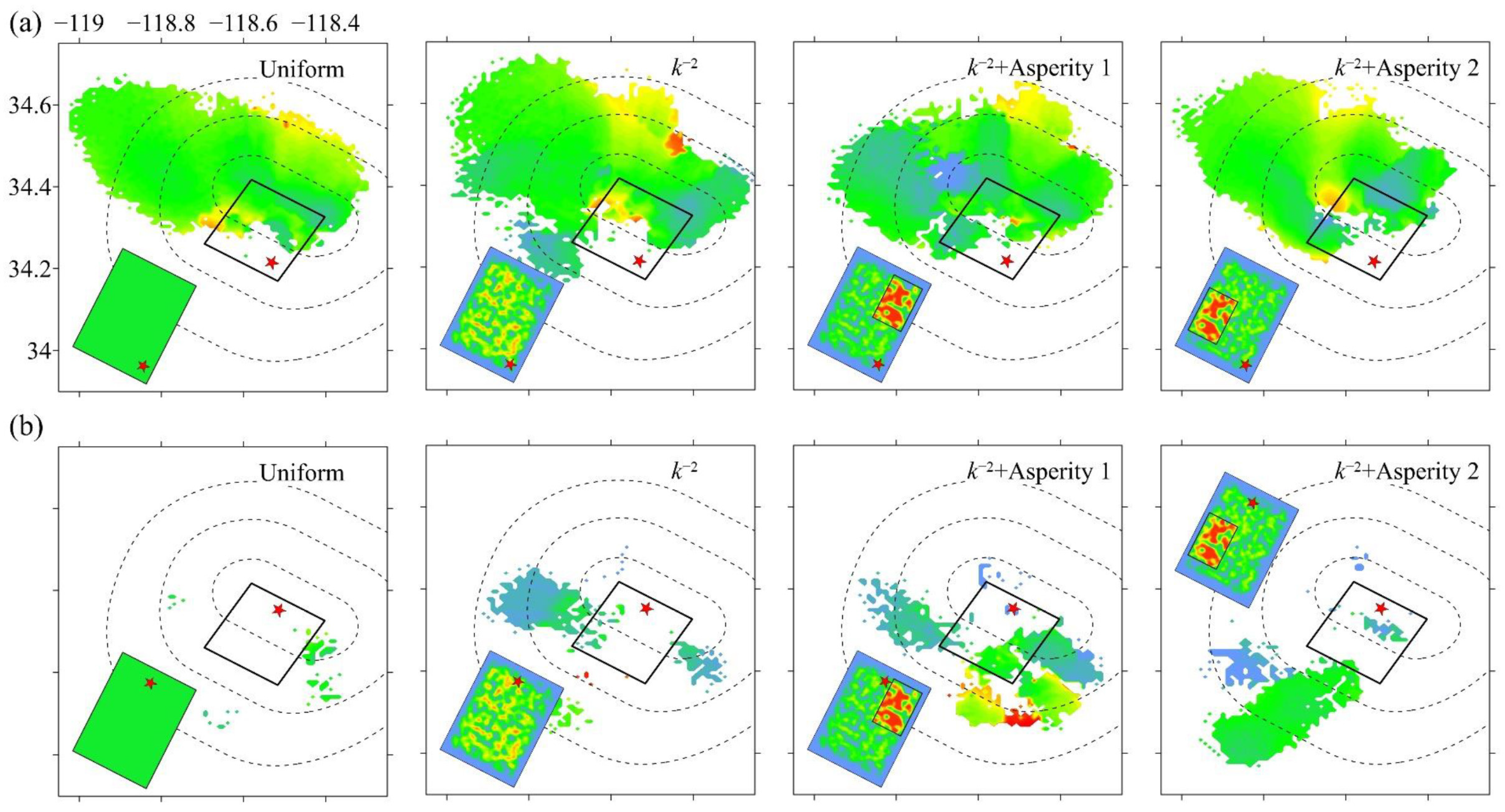
5. Influence of Slip Distribution on Area of Near-Fault Pulses

5.1. Type of Slip Distribution

It is incredibly difficult to predict the nonuniform slip distribution on the fault plane for an event from existing knowledge regarding the earthquake source. Currently, the development of pulse models ignores the effect of nonuniformity of slip and mainly emphasizes the rupture directivity effect. The slip distribution has a great influence on near-fault ground motion and thus on the spatial distribution of pulses. This section investigates how the pulse area varies for different types of slip distributions and the implication on the improvement of pulse models.

Based on the source models of the two earthquakes, this section sets three types of slip distributions: the uniform slip, the random k⁻² slip [40], and the hybrid slip that combines the deterministic asperity slip with the random k⁻² slip [25]. The random slip with the k⁻² wavenumber spectrum can be generated by the following equation [22,25]

$$D(k_x,k_y)={\displaystyle \frac{\overline{D}\cdot L\cdot W}{\sqrt{1+{\left[{\left(k_x/k_{cx}\right)}^2+{\left(k_y/k_{cy}\right)}^2\right]}^2}}}\exp \left(i\Psi (k_x,k_y)\right)$$

(6)

where $k_x$ and $k_y$ are the wavenumbers along strike and down dip, respectively; $k_{cx}$ and $k_{cy}$ are the corresponding corner wavenumbers; and $\Psi (k_x,k_y)$ is the random phase.

For the hybrid slip model, one asperity is set on the fault plane at a shallow position or at a deep position. The four kinds of slip distribution are shown in Figure 11 for the two earthquakes. To have different propagation effects, the hypocenter is set at two positions: the bottom right corner of the fault for the unilateral rupture, and the middle of the upper edge of the fault for the bilateral rupture. In total, eight source rupture models are adopted for each earthquake.

5.2. Influence of Slip Distribution

Similar to Section 3, the ground motion field is simulated using the FK approach and then the pulse area is determined by SB14 for each of source rupture models. Figure 12 and Figure 13 show the pulse area filled by the pulse period for the Imperial Valley and the Northridge earthquakes, respectively. Note that Figure 12 and Figure 13 use a smaller scope of the map to concentrate on the variation of pulse area, and adopt the same color scales for the slip distribution and the pulse period.

Figure 12 and Figure 13 indicate that the rupture propagation effect controls the basic distribution pattern of the pulse area, and the slip distribution has a great influence on the pulse area. The presence of asperity makes the center of the pulse area closer to the asperity. The pulse areas for the unilateral and bilateral ruptures are quite different due to the strong propagation effect. For the strike-slip earthquake, the uniform slip causes the pulse area along the fault trace, and the uniformity of the slip leads to a large discontinuity of the pulse area. While for the dip-slip earthquake, the influence of the propagation effect on the pulse area is very large. The area near the rupture end is concentrated up dip from the hypocenter for the unilateral rupture, and thus large pulses occur.

Due to the influence of asperity, a pulse occurs in many near-fault regions that are weakly affected by the rupture directivity effect. As the directivity and nondirectivity pulses have no objective boundary [13], it is hard to separate the pulse area by whether it is caused by the rupture directivity effect manually. This means that the pulse model developed only using the directivity pulse may underestimate the occurrence probability of pulses. Thus, the directivity and nondirectivity pulses should be pooled together to establish the pulse model. The spatial distribution of pulse period is also affected by slip distribution, but some key features are preserved. One prominent phenomenon is that for a given hypocenter, the area with a large pulse period has little variation with slip distribution. This may lead to a conclusion that the asperity mainly affects the pulse amplitude while the source-to-site geometry influences the pulse period. This feature could be considered in the estimation model of the pulse period.

6. Conclusions

To provide a suitable ground motion input for the seismic resistance of building structures, this study performs spatial characteristic analysis of the near-fault velocity pulse based on simulated ground motion fields. The Mw 6.58 strike-slip Imperial Valley earthquake and the Mw 6.8 dip-slip Northridge earthquake are adopted as the cases due to the rich pulse-like records. The ground motion simulation method based on the frequency–wavenumber Green’s function is applied. Comparisons of velocity time history, response spectra, and peak value indicate that the FK approach can provide a good estimation of ground motion and reproduce the pulse characteristics as expressed in the observed records. The multi-component broadband ground motion fields in the calculation area with a size of 120 km × 120 km are simulated for the two earthquakes, and the pulse parameters and pulse area are extracted using the multi-component pulse identification method. For the two earthquakes, the pulse area of the simulated ground motion field accords well with the spatial distribution of pulse-like and non-pulse-like records.

Then, the spatial characteristic analyses are performed for various pulse parameters, including the pulse period, the pulse amplification factor, and the orientation of the maximum component. We find that the pulse period for an earthquake is not a constant but a spatial variable related to source-to-site geometry, and the spatial distribution for the dip-slip earthquake is more complex than that for the strike-slip case. The pulse amplification factor has great spatial variation, and this is related to the fault geometry. The orientation of the maximum pulse component is not the FN component in most cases, and even the FN component is not in the orientations that exhibit pulse, especially for the dip-slip earthquake. This study concludes that the radiation pattern controlled by the seismic source mechanism determines the orientation of the maximum component. The pulse amplification factor exhibits slight change with the orientation of the maximum pulse component and has similar performance to the previous empirical statistical models.

Based on the two earthquakes, the influence of slip distribution on pulse area is investigated. The uniform slip, the random slip, and the hybrid slip with two different locations of asperity are combined with the unilateral rupture and the bilateral rupture to build eight source rupture models for each earthquake. It is found that the rupture propagation effect controls the basic distribution pattern of pulse area, and the slip distribution has great influence. The presence of asperity makes the pulse area closer to the asperity, and the nonuniformity of slip leads to a large discontinuity of the pulse area. Additionally, the slip distribution has a weaker influence on the pulse period distribution than the source-to-site geometry. The results of this study are beneficial to the future improvements of pulse prediction models in probabilistic seismic hazard analysis and ground motion input for structural seismic analysis.

Note that these findings are obtained based on a typical strike-slip earthquake and a typical dip-slip event. It is meaningful to expand the research to more diverse earthquake cases with larger magnitudes (e.g., the 2023 Mw 7.8 and Mw 7.5 Turkey earthquake sequence, and the 2025 Mw 7.7 Myanmar earthquake). In addition, the simulation of various earthquake scenarios does not consider the soil-site effect, and further study is required on the influence of site conditions on the velocity pulse.

References

1. Shahi, S.K.; Baker, J.W. An Empirically Calibrated Framework for Including the Effects of Near-Fault Directivity in Probabilistic Seismic Hazard Analysis. Bull. Seismol. Soc. Am. 2011, 101, 742–755. [Google Scholar] [CrossRef]
2. Chioccarelli, E.; Iervolino, I. Near-Source Seismic Hazard and Design Scenarios. Earthq. Eng. Struct. Dyn. 2013, 42, 603–622. [Google Scholar] [CrossRef]
3. Withers, K.; Moschetti, M.; Powers, P.; Petersen, M.; Graves, R.; Aagaard, B.T.; Baltay, A.; Luco, N.; Wirth, E.; Rezaeian, S.; et al. Integration of Rupture Directivity Models for the US National Seismic Hazard Model. Earthq. Spectra 2024, 40, 1066–1098. [Google Scholar] [CrossRef]
4. Iervolino, I.; Cornell, C.A. Probability of Occurrence of Velocity Pulses in Near-Source Ground Motions. Bull. Seismol. Soc. Am. 2008, 98, 2262–2277. [Google Scholar] [CrossRef]
5. Estacio, J.L.P.; De Risi, R. Historical Evolution of the Input Parameters of Ergodic and Non-Ergodic Ground Motion Models (GMMs): A Review. Earth-Sci. Rev. 2025, 105074. [Google Scholar] [CrossRef]
6. Spudich, P.; Bayless, J.; Baker, J.; Chiou, S.; Somerville, A. Final Report of the NGA-West2 Directivity Working Group; Pacific Earthquake Engineering Research Center (PEER): Berkeley, CA, USA, 2013. [Google Scholar]
7. Weatherill, G.; Lilienkamp, H. Capturing Directivity in Probabilistic Seismic Hazard Analysis for New Zealand: Challenges, Implications, and a Machine Learning Approach for Implementation. Bull. Seismol. Soc. Am. 2024, 114, 373–398. [Google Scholar] [CrossRef]
8. Somerville, P.G. Magnitude Scaling of the near Fault Rupture Directivity Pulse. Phys. Earth Planet. Inter. 2003, 137, 201–212. [Google Scholar] [CrossRef]
9. Bayless, J.; Abrahamson, N.A.; Somerville, P.G. A Rupture Directivity Adjustment Model and Its Application in Seismic Hazard. Earthq. Spectra 2025, 41, 753–781. [Google Scholar] [CrossRef]
10. Xie, J.; Li, X.; Wen, Z. The Amplification Effects of Near-Fault Distinct Velocity Pulses on Response Spectra. Eng. Mech. 2017, 34, 194–211. [Google Scholar]
11. Chang, Z.; Sun, X.; Zhai, C.; Zhao, J.X.; Xie, L. An Empirical Approach of Accounting for the Amplification Effects Induced by Near-Fault Directivity. Bull. Earthq. Eng. 2018, 16, 1871–1885. [Google Scholar] [CrossRef]
12. Chang, Z.; Wu, H.; Goda, K. Automated Parameterization of Velocity Pulses in Near-fault Ground Motions. Earthq. Eng. Struct. Dyn. 2024, 53, 1006–1027. [Google Scholar] [CrossRef]
13. Shahi, S.K.; Baker, J.W. An Efficient Algorithm to Identify Strong-Velocity Pulses in Multicomponent Ground Motions. Bull. Seismol. Soc. Am. 2014, 104, 2456–2466. [Google Scholar] [CrossRef]
14. Withers, K.B.; Olsen, K.B.; Day, S.M.; Shi, Z. Ground Motion and Intraevent Variability from 3D Deterministic Broadband (0–7.5 Hz) Simulations along a Nonplanar Strike-Slip Fault. Bull. Seismol. Soc. Am. 2019, 109, 229–250. [Google Scholar] [CrossRef]
15. Dadras, E.Y.; Yazdani, A.; Nicknam, A.; Eftekhari, S.N. Incorporating Source Rupture Characteristics into the Near-Fault Pulse Prediction Model. Bull. Seismol. Soc. Am. 2018, 108, 200–209. [Google Scholar] [CrossRef]
16. Somerville, P.G.; Smith, N.F.; Graves, R.W.; Abrahamson, N.A. Modification of Empirical Strong Ground Motion Attenuation Relations to Include the Amplitude and Duration Effects of Rupture Directivity. Seismol. Res. Lett. 1997, 68, 199–222. [Google Scholar] [CrossRef]
17. Rowshandel, B. Incorporating Source Rupture Characteristics into Ground-Motion Hazard Analysis Models. Seismol. Res. Lett. 2006, 77, 708–722. [Google Scholar] [CrossRef]
18. Yu, H.; Zhu, C.; Chen, Q. Intelligent Identification Method for Pulse-like Ground Motions and Field Distribution of Three-Dimensional Orientation-Independent Pulse Characteristics. Soil Dyn. Earthq. Eng. 2024, 182, 108722. [Google Scholar] [CrossRef]
19. Lin, Y.Y.; Kanamori, H.; Zhan, Z.; Ma, K.F.; Yeh, T.Y. Modelling of Pulse-like Velocity Ground Motion during the 2018 Mw6.3 Hualien Earthquake, Taiwan. Geophys. J. Int. 2020, 223, 348–365. [Google Scholar] [CrossRef]
20. Yen, M.H.; von Specht, S.; Lin, Y.Y.; Cotton, F.; Ma, K.F. Within-and Between-Event Variabilities of Strong-Velocity Pulses of Moderate Earthquakes within Dense Seismic Arrays. Bull. Seismol. Soc. Am. 2022, 112, 361–380. [Google Scholar] [CrossRef]
21. Han, L.; Tao, Z.; Cao, Z.; Tao, X. Relationship Between Asperities and Velocity Pulse Generation Mechanism. Front. Earth Sci. 2022, 10, 843532. [Google Scholar] [CrossRef]
22. Cao, Z.; Tao, X.; Tao, Z.; Tang, A. Kinematic Source Modeling for the Synthesis of Broadband Ground Motion Using the F-k Approach. Bull. Seismol. Soc. Am. 2019, 109, 1738–1757. [Google Scholar] [CrossRef]
23. Hartzell, S.; Liu, P.; Mendoza, C.; Ji, C.; Larson, K.M. Stability and Uncertainty of Finite-Fault Slip Inversions: Application to the 2004 Parkfield, California, Earthquake. Bull. Seismol. Soc. Am. 2007, 97, 1911–1934. [Google Scholar] [CrossRef]
24. Zhu, L.; Rivera, L.A. A Note on the Dynamic and Static Displacements from a Point Source in Multilayered Media. Geophys. J. Int. 2002, 148, 619–627. [Google Scholar] [CrossRef]
25. Gallovič, F.; Brokešová, J. On Strong Ground Motion Synthesis with k−2 Slip Distributions. J. Seismol. 2004, 8, 211–224. [Google Scholar] [CrossRef]
26. Crempien, J.G.F.; Archuleta, R.J. UCSB Method for Simulation of Broadband Ground Motion from Kinematic Earthquake Sources. Seismol. Res. Lett. 2015, 86, 61–67. [Google Scholar] [CrossRef]
27. Baker, J.W. Quantitative Classification of Near-Fault Ground Motions Using Wavelet Analysis. Bull. Seismol. Soc. Am. 2007, 97, 1486–1501. [Google Scholar] [CrossRef]
28. Hartzell, S.H.; Heaton, T.H. Inversion of Strong Ground Motion and Teleseismic Waveform Data for the Fault Rupture History of the 1979 Imperial Valley, California, Earthquake. Bull. Seismol. Soc. Am. 1983, 73, 1553–1583. [Google Scholar] [CrossRef]
29. Wald, D.J.; Heaton, T.H.; Hudnut, K.W. The Slip History of the 1994 Northridge, California, Earthquake Determined from Strong-Motion, Teleseismic, GPS, and Leveling Data. Bull. Seismol. Soc. Am. 1996, 86, S49–S70. [Google Scholar] [CrossRef]
30. Cao, Y.; Mavroeidis, G.P. Simulation of Near-Fault Ground Strains and Rotations from Actual Strike-Slip Earthquakes: Case Studies of the 2004 Mw 6.0 Parkfield, the 1979 Mw 6.5 Imperial Valley and the 1999 Mw 7.5 Izmit Earthquakes. Geophys. J. Int. 2021, 226, 1920–1947. [Google Scholar] [CrossRef]
31. Luo, Q.; Zhang, G.; Ding, B.; Ji, Z. Evaluation of Strongest Ground Motions under Strike-Slip Rupture for the Luding and Imperial Valley Earthquakes. Soil Dyn. Earthq. Eng. 2025, 194, 109390. [Google Scholar] [CrossRef]
32. Hough, S.E.; Graves, R.W.; Cochran, E.S.; Yoon, C.E.; Blair, L.; Haefner, S.; Wald, D.J.; Quitoriano, V. The 17 January 1994 Northridge, California, Earthquake: A Retrospective Analysis. Seism. Rec. 2024, 4, 151–160. [Google Scholar] [CrossRef]
33. McGarr, A.; Fletcher, J. Mapping Apparent Stress and Energy Radiation over Fault Zones of Major Earthquakes. Bull. Seismol. Soc. Am. 2002, 92, 1633–1646. [Google Scholar] [CrossRef]
34. Graves, R.W.; Pitarka, A. Broadband Ground-Motion Simulation Using a Hybrid Approach. Bull. Seismol. Soc. Am. 2010, 100, 2095–2123. [Google Scholar] [CrossRef]
35. Ancheta, T.D.; Darragh, R.B.; Stewart, J.P.; Seyhan, E.; Silva, W.J.; Chiou, B.S.-J.; Wooddell, K.E.; Graves, R.W.; Kottke, A.R.; Boore, D.M.; et al. NGA-West2 Database. Earthq. Spectra 2014, 30, 989–1005. [Google Scholar] [CrossRef]
36. Boore, D.M.; Stewart, J.P.; Seyhan, E.; Atkinson, G.M. NGA-West2 Equations for Predicting PGA, PGV, and 5% Damped PSA for Shallow Crustal Earthquakes. Earthq. Spectra 2014, 30, 1057–1085. [Google Scholar] [CrossRef]
37. Pitarka, A.; Graves, R.; Irikura, K.; Miyakoshi, K.; Wu, C.; Kawase, H.; Rodgers, A.; McCallen, D. Refinements to the Graves–Pitarka Kinematic Rupture Generator, Including a Dynamically Consistent Slip-Rate Function, Applied to the 2019 Mw 7.1 Ridgecrest Earthquake. Bull. Seismol. Soc. Am. 2022, 112, 287–306. [Google Scholar] [CrossRef]
38. Boore, D.M. Orientation-Independent, Nongeometric-Mean Measures of Seismic Intensity from Two Horizontal Components of Motion. Bull. Seismol. Soc. Am. 2010, 100, 1830–1835. [Google Scholar] [CrossRef]
39. Howard, J.K.; Tracy, C.A.; Burns, R.G. Comparing Observed and Predicted Directivity in Near-Source Ground Motion. Earthq. Spectra 2005, 21, 1063–1092. [Google Scholar] [CrossRef]
40. Somerville, P.; Irikura, K.; Graves, R.; Sawada, S.; Wald, D.; Abrahamson, N.; Iwasaki, Y.; Kagawa, T.; Smith, N.; Kowada, A. Characterizing Crustal Earthquake Slip Models for the Prediction of Strong Ground Motion. Seismol. Res. Lett. 1999, 70, 59–80. [Google Scholar] [CrossRef]
41. Takenaka, H.; Mamada, Y.; Futamure, H. Near-Source Effect on Radiation Pattern of High-Frequency S Waves: Strong SH-SV Mixing Observed from Aftershocks of the 1997 Northwestern Kagoshima, Japan, Earthquakes. Phys. Earth Planet. Inter. 2003, 137, 31–43. [Google Scholar] [CrossRef]
42. Castro, R.; Franceschina, G.; Pacor, F.; Bindi, D.; Luzi, L. Analysis of the Frequency Dependence of the S-Wave Radiation Pattern from Local Earthquakes in Central Italy. Bull. Seismol. Soc. Am. 2006, 96, 415–426. [Google Scholar] [CrossRef]
43. Takemura, S.; Furumura, T.; Saito, T. Distortion of the Apparent S-Wave Radiation Pattern in the High-Frequency Wavefield: Tottori-Ken Seibu, Japan, Earthquake of 2000. Geophys. J. Int. 2009, 178, 950–961. [Google Scholar] [CrossRef]
44. Sandeep; Joshi, A.; Kamal; Kumar, P.; Kumar, A. Effect of Frequency-Dependent Radiation Pattern in the Strong Motion Simulation of the 2011 Tohoku Earthquake, Japan, Using Modified Semi-Empirical Method. Nat. Hazards 2014, 73, 1499–1521. [Google Scholar] [CrossRef]
45. Li, C.; Zuo, Z.; Kunnath, S.; Chen, L. Orientation of the Strongest Velocity Pulses and the Maximum Structural Response to Pulse-like Ground Motions. Soil Dyn. Earthq. Eng. 2020, 136, 106240. [Google Scholar] [CrossRef]
Figure 1. Model bias and standard deviation (SD) of PSA, PGA, and PGV for (a) the Imperial Valley earthquake and (b) the Northridge earthquake. Comparison of the observed and synthetic PGV with the GMPE estimates versus the Joyner–Boore distance, for (c) the Imperial Valley earthquake and (d) the Northridge earthquake.
Buildings 15 01363 g001
Figure 2. Comparison of the observed and synthetic PSA of the maximum component at 10 selected stations for (a) the Imperial Valley earthquake and (b) the Northridge earthquake. The dashed line indicates the pulse period, and the record sequence number is shown for each station.
Buildings 15 01363 g002
Figure 3. Comparison of the observed and synthetic velocity time histories at six stations for the Northridge earthquake. The record sequence number is shown for each station.
Buildings 15 01363 g003
Figure 4. (a) Pulse area and (b) PGV distribution of the synthetic ground motion field for the Imperial Valley earthquake; (c,d) are the same for the Northridge earthquake. The dots denote the pulse identification results and PGV of the observed records, and the dashed line represents the contour of rupture distance of 40 km. The thick line and star represent the projection of the fault plane and hypocenter, respectively. The slip distribution in the bottom left corner is viewed at 233° and 212° and from the north for the Imperial Valley and Northridge earthquakes, respectively. The arrows express the rake angle.
Buildings 15 01363 g004
Figure 5. Spatial distributions of (a) the pulse period and (b) the amplification factor at the pulse period for the Imperial Valley earthquake; (c,d) are the same for the Northridge earthquake. The thick line and star represent the projection of the fault plane and hypocenter, respectively.
Buildings 15 01363 g005
Figure 6. Illustration of the orientations of the maximum component (α) and half of the orientation range that exhibits pulse (β).
Buildings 15 01363 g006
Figure 7. Spatial distributions of (a) α, (b) R FN ( 0.3   Hz ) , and (c) β in the synthetic ground motion field for the Imperial Valley earthquake; (df) are the same for the Northridge earthquake. The thick line and star represent the projection of the fault plane and hypocenter, respectively.
Buildings 15 01363 g007
Figure 8. Pulse amplification factor in different ranges of α in the synthetic ground motion field for the two earthquakes, along with previous models (Shahi and Baker [1], Xie et al. [10], and Chang et al. [11]).
Buildings 15 01363 g008
Figure 9. Pulse amplification factor at different ranges of α for the 175 pulse-like records, along with previous models (Shahi and Baker [1], Xie et al. [10], and Chang et al. [11]).
Buildings 15 01363 g009
Figure 10. Distribution of β with α for the 175 pulse-like records. The shaded area indicates β < α .
Buildings 15 01363 g010
Figure 11. The uniform slip, the random k−2 slip, and the hybrid slip (k−2 + asperity) generated for (a) the Imperial Valley and (b) the Northridge earthquakes. The colorbars of slip distributions are the same as in Figure 4, and the black frame indicates the location of asperity.
Buildings 15 01363 g011
Figure 12. Pulse area and pulse period from the uniform slip, the k−2 slip, and the hybrid slip (k−2 + asperity) with (a) the unilateral rupture and (b) the bilateral rupture, for the Imperial Valley earthquake. The dashed line indicates the contour of the rupture distance with an interval of 10 km. The thick line and star represent the projection of the fault plane and hypocenter, respectively. The colorbars for slip distribution and pulse period are the same as those in Figure 4 and Figure 5, respectively.
Buildings 15 01363 g012
Figure 13. The same as Figure 12, but for the Northridge earthquake.
Buildings 15 01363 g013