Study on the Engineering Characteristics of Alluvial Silty Sand Embankment Under Vehicle Loads

Abstract

This article takes alluvial silty sand in the alluvial plain area as the research object. Through a combination of theoretical analysis, finite element simulation, and on-site testing, the engineering characteristics of alluvial silty sand under traffic loads, as well as the feasibility of using alluvial silty sand as roadbed filling material in practical engineering, are systematically expounded on for the first time. The research results indicate that the influence of vehicle speed on the distribution and depth of dynamic stress is relatively small, while the moisture content (optimal 7.8%) and compaction degree (>94%) are the key factors determining the performance of the roadbed. Specifically, the displacement at the top of the roadbed varies with changes in moisture content. An increase in compaction degree is beneficial for reducing settlement and enhancing the stability of the roadbed. Through comparative analysis of finite element simulation and on-site testing, it was found that although the initial settlement of alluvial silt filling is large, the settlement rate is fast and can stabilize in a short period of time. Its long-term performance can still meet engineering requirements. Research has shown that alluvial silt can be used as an economical and reasonable roadbed filling material, but in practical applications, strict control of moisture content and compaction degree is required to optimize roadbed performance.

1. Introduction

In the alluvial plain area, alluvial silty sand is widely distributed, with complex causes [1,2], fine particles, and unstable deformation under dynamic loads, making it special in engineering applications. When constructing roadbeds, on-site soil sampling can effectively reduce resource waste and construction costs. With the development of heavy-load traffic and highways, further exploration of the engineering characteristics of sandy soil as roadbed filling under traffic loads has become one of the current research directions.

Alluvial silty sand is transported by water flow. Due to its small particle size and uniform gradation, it exhibits high porosity, good permeability, low bearing capacity, and significant variability in shear strength [3,4,5,6,7,8]. Under the influence of traffic loads, it faces more complex engineering challenges. Xu et al. [9] quantitatively analyzed the impact of pore structure on the early mechanical properties and durability of foam concrete, providing important references for the study of mechanical behavior in similar porous materials. Scholars such as Dai have found that at low vehicle speeds, traffic loads approximate static loads. As speed increases, the stresses and displacements generated by traffic loads exhibit different dynamic cyclic characteristics depending on the pavement structure, and similar characteristics have been observed in the subgrade structure [10,11]. The dynamic properties of soil can be described by various parameter relationships, showing hysteresis, softening, and nonlinearity under dynamic loading. Dynamic stress–strain characteristics are generally described using elastoplastic and viscoelastic models [12,13,14,15]. The dynamic elastic modulus changes with confining pressure and the degree of consolidation, decreasing with increasing strain amplitude, while the damping ratio shows a trend opposite to that of the dynamic elastic modulus [16,17]. As moisture content increases, the critical dynamic stress of compacted silty sand shows a linear decreasing trend [18,19]. Kenji Ishihara [20,21], Andrzej S. Nowak [22], and others have also proposed new dynamic soil models.

So far, a large number of scholars have studied the engineering properties of soil, but there is still insufficient research on the characteristics of alluvial silt under vehicle loads. Most existing research focuses on the establishment of theoretical models and the analysis of experimental data, with insufficient understanding of the actual behavior (especially long-term performance) of vehicles under dynamic loads. There is also a lack of verification research combining on-site monitoring and numerical simulation, as well as a lack of engineering guidance on controlling moisture content and compaction degree. Based on this, this article explores the influence of various factors on the settlement and dynamic stress level of alluvial silty sand subgrade at different depths under dynamic loads through theoretical analysis of dynamic stress propagation laws, finite element simulation (ANSYS 2020R2) to examine multifactor coupling effects, and field tests on the Chicao Expressway (K49 + 534.7 section). The engineering behavior of alluvial silty sand subgrade as a filler under vehicle dynamic loads is analyzed, aiming to provide a valuable reference for practical engineering projects.

2. Analytical Basis

2.1. Simplification of Vehicle Load

To investigate the characteristics of alluvial silty sand subgrade under vehicle dynamic loads and optimize numerical calculation efficiency, it is necessary to reasonably simplify the vehicle load. Different types of vehicle models have varying simplification methods, leading to differences in simulation results.

The dynamic loads generated by vehicles during operation come in various forms, including constant loads, periodic harmonic loads, transient impact loads, and randomly distributed loads [23,24]. Among these types of loads, mobile harmonic loads have attracted much attention due to their widespread existence. In addition, common simplification methods for vehicle dynamic loads include the moving constant load method, multi-axis vibration model, and quarter-vehicle harmonic load model. The quarter-vehicle model shown in Figure 1 is not only commonly used for such loads but also has the following advantages compared to other methods: Compared with multi-axial models, this approach reduces the number of elements by 40% while maintaining over 90% accuracy in stress distribution [25]; it better reflects the coupling effect between tire damping and soil, which is crucial for porous silt [26], and has been successfully applied in similar granular roadbed research [27,28].

By comprehensively analyzing these factors, the dynamic load characteristics of the vehicle can be expressed as a sine function based on the quarter-vehicle model (Formula (1)), where k₁ is the equivalent suspension stiffness of the vehicle, b₁ is the damping coefficient of the vehicle suspension system, p₀ is the static wheel load, and ω is the vibration angular frequency. Formula (2) further simplifies the peak dynamic load to p(t) = (1 + δ)p₀, where δ is the dynamic impact coefficient. This simplified method is consistent with on-site measured data and balances computational efficiency and accuracy.

$$p\left(t \right)=k_1{b}_{1}sin\left(\omega t+\theta \right)+p_0$$

(1)

$$p\left(t \right)=(1+\delta )p_0$$

(2)

Although the quarter-vehicle model can effectively reflect the basic dynamic interactions, subsequent research can incorporate the influence of the wheelbase (usually 3–5 m for heavy-load vehicles) to refine specific frequency responses. Within the scope of this study, the sine load (Formula (1)) covers the dominant frequency components of highway traffic (1–5 Hz, corresponding to typical wheelbase configurations at speeds of 30–90 km/h).

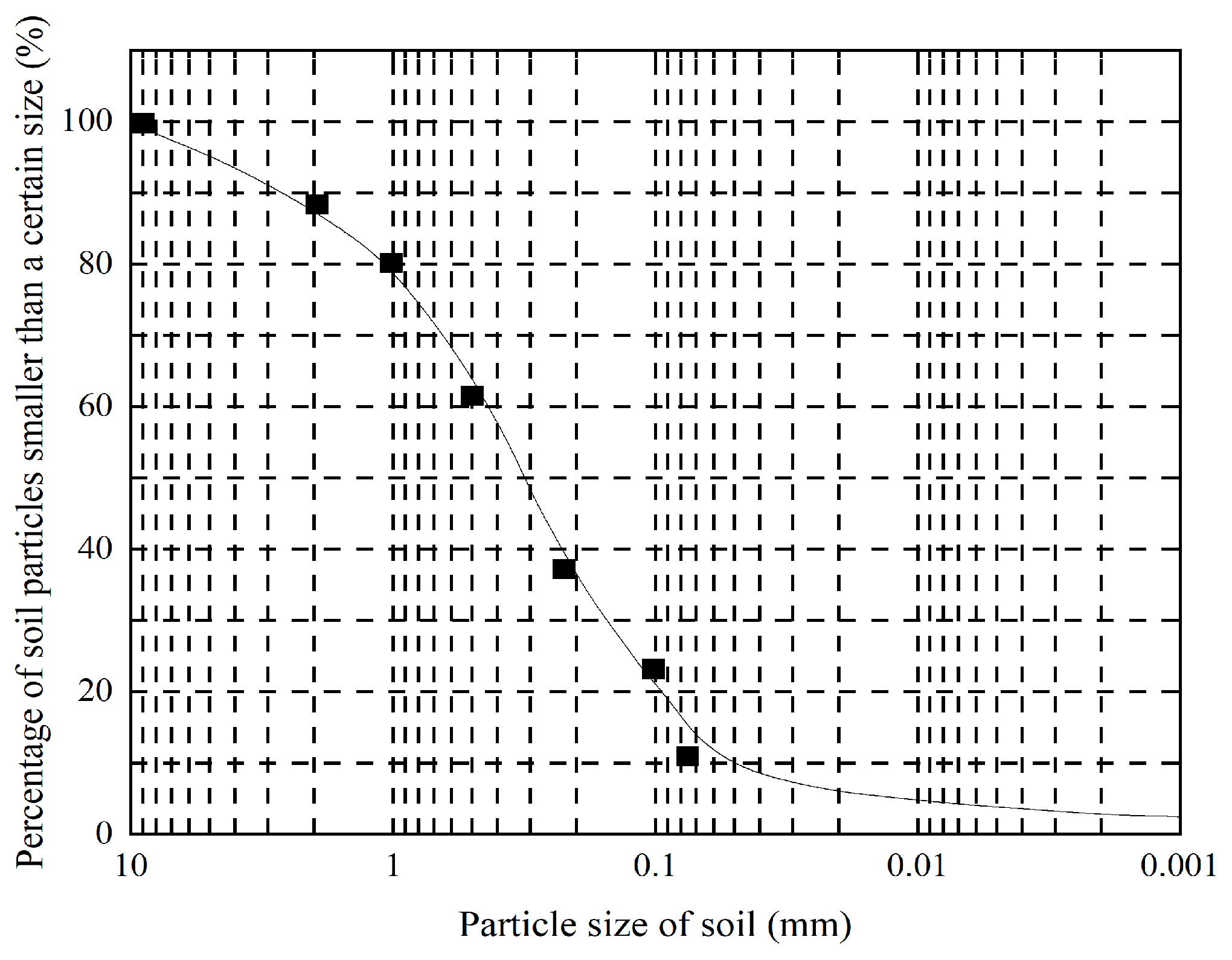
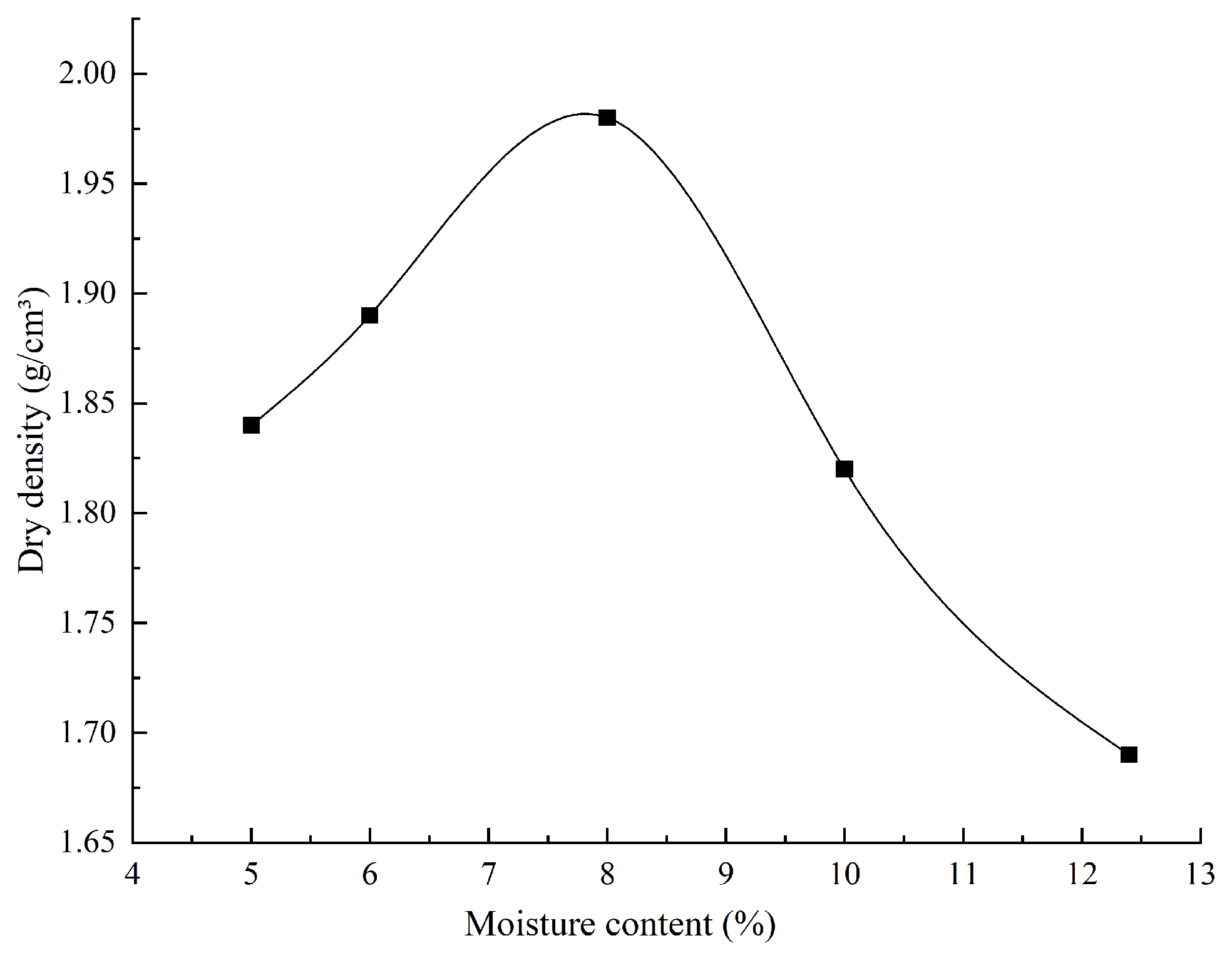
2.2. Basic Soil Properties

The alluvial silty sand was taken from the Luanqing section of the Chicao Expressway. According to the ASTM D2487 standard [29], due to the fine particle content (<0.075 mm) of 4.6% and plasticity index (Ip) of 2.62, the soil is classified as SM (silty sand), which is consistent with the “Engineering Classification Standard for Soil” (GB/T 50145-2007 [30]). Use a thin-walled soil sampler to take samples at a depth of 0.5–1.2 m, and remove visible roots/gravel (>5 mm) on site. When selecting samples, ensure consistency in grading and that organic matter content is less than 1%. Analyze soil properties using methods such as particle size grading test, limit moisture content test, and compaction test.

Particle Size Grading Test: The air-dried soil sample is sieved through a 2 mm sieve, and according to ASTM D6913-17 [31], the distribution characteristics of different particle sizes of alluvial silt sand are clarified, that is, the particle size distribution of soil. The analysis results are as follows

Table 1. Particle size analysis results.

Size/mm	>2	2~1	1~0.5	0.5~0.25	0.25~0.075	<0.075
Distribution	11.9%	11%	17.8%	26.9%	27.8%	4.6%

and Figure 2:

The coefficient of uniformity (Cu) is 7.43, which is greater than 5, and the coefficient of curvature (Cc) is 2.42, falling within the range of 1 < Cc < 3. These values indicate that the particle size distribution of the sampled soil is well graded.

Limit Moisture Content Test: According to ASTM D4318-17 [32], tests were conducted on the alluvial silty sand of the Chicao Expressway section to determine WL, WP, and Ip. The results are shown in

Table 2. Atterberg limits test results.

Parameter	Liquid Limit (WL, %)	Plastic Limit (WP, %)	Plasticity Index (Ip)
Value	29.6	8.4	2.62

.

Compaction Test: The standard Proctor compaction method (ASTM D698-12 [33]) has a compaction energy of 600 kN∙m/m³ and is compacted in 3 layers, with 25 blows per layer. As shown in Figure 3, dry density varies with changes in moisture content. The dry density of the soil sample reaches its peak value at a moisture content of 7.8%.

3. Dynamic Triaxial Test Study

The experiment used GDS dynamic triaxial testing equipment to test the stress–strain fitting and dynamic elastic modulus–dynamic strain fitting relationship of the sample soil. When selecting the testing conditions, the confining pressure was chosen to cover the typical range of road subgrade overburden pressure (JTG D30-2015 [34]). Considering 8% as the optimal value for the compaction test, 6% and 10% cover the natural fluctuation range measured on the Chicao Expressway. Considering that the main frequency of vibration for heavy-duty trucks (dominant traffic load) is 2.3 ± 0.8 Hz and most vehicles have vibration frequencies less than 5 Hz, the frequency range was determined accordingly.

3.1. Test Equipment

The GDS dynamic triaxial testing equipment used in this experiment is shown in Figure 4. The GDS dynamic triaxial tester can apply a maximum dynamic axial load of ±10 kN, with a frequency range of 0–5 Hz and an accuracy of 0.1%. The selected frequency range (1–5 Hz) corresponds to the main frequency of typical highway traffic loads. For vehicles with a wheelbase of 3–5 m and a speed of 60 km per hour (16.67 m per second), the basic excitation frequency is calculated to be 3.3–5.6 Hz (f = vehicle speed/wheelbase). This setting ensures that the experiment effectively simulates actual operating load conditions. The maximum deformation of the sample is 100 mm, the displacement resolution is 0.208 mm, and the accuracy is 0.07% of the interval. It can simulate waveforms, such as triangular waves, sine waves, normal waves, square waves, trapezoidal waves, and oblique waves. The experiment uses standard cylindrical specimens (50 mm in diameter × 100 mm in height).

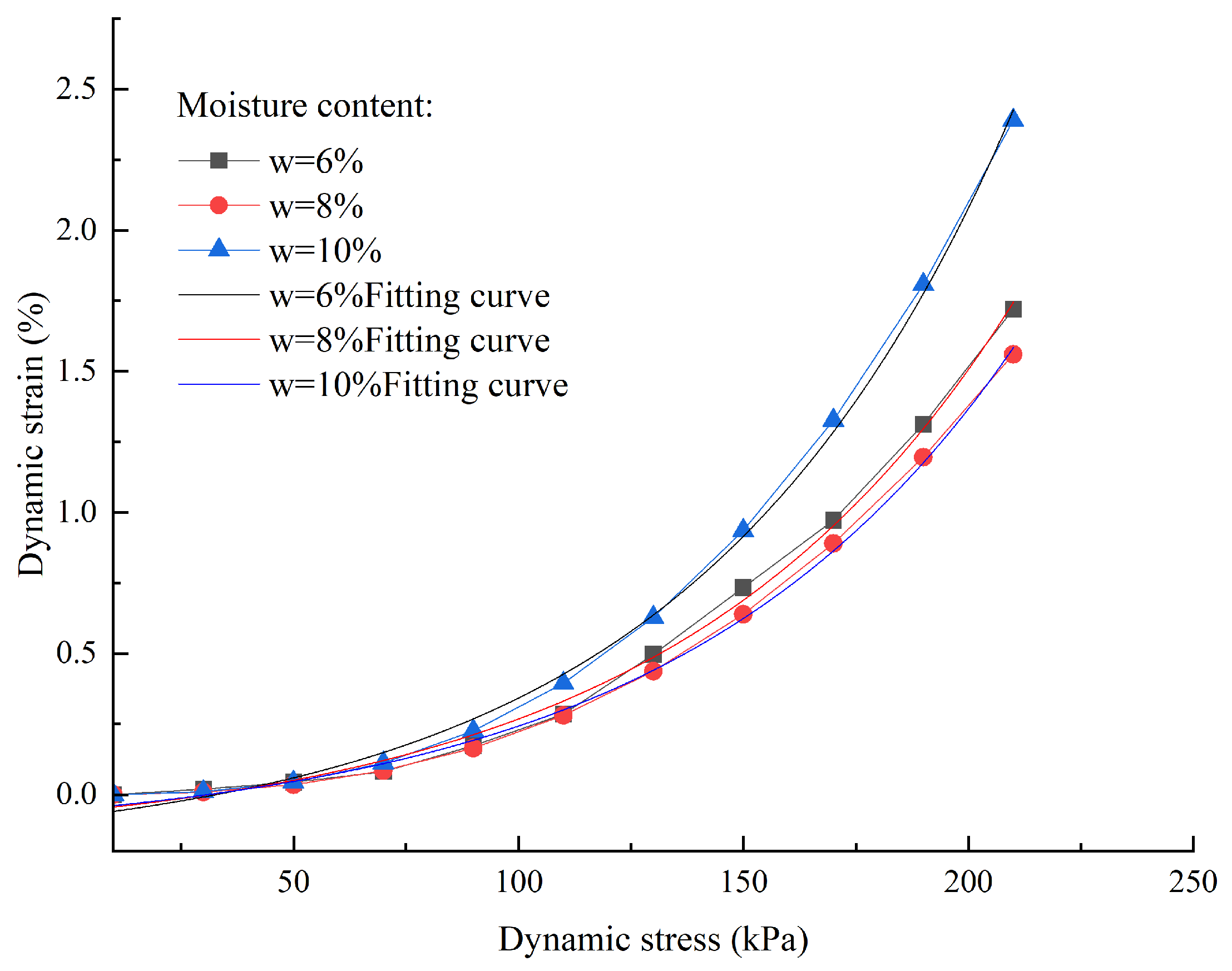
3.2. Stress–Strain Fitting of Soil Samples

The dynamic strain of the soil sample exhibits a curvilinear increase with stress, and this relationship can be described using the R.L. Kondner hyperbolic model [35]:

$${\sigma }_d={\displaystyle \frac{{\epsilon }_d}{a+b{\epsilon }_d}}$$

(3)

In the equation, ${\sigma }_d$ is the dynamic stress, ${\epsilon }_d$ is the dynamic strain, and a and b are fitted material constants. Similarly, Wang et al. [36] investigated the creep characteristics of coral sand and proposed a dynamic constitutive model suitable for granular materials, offering significant insights into the mechanical behavior of alluvial silty sand under dynamic loads.

Table 3. Parameters of dynamic stress–strain curves for alluvial silty sand under different conditions.

No.	Confining Pressure (kPa)	Moisture Content (%)	a	b	R2
1	30	8	8.47 × 10−6	4.31 × 10−3	0.9686
2	50	8	6.32 × 10−6	6.32 × 10−3	0.9535
3	80	8	5.19 × 10−6	7.12 × 10−3	0.969
4	50	6	6.89 × 10−6	6.73 × 10−3	0.9578
5	50	10	7.64 × 10−6	4.69 × 10−3	0.9610

shows the values of these parameters and $R^2$ under different test conditions. Taking moisture content as an example, under the condition of a constant confining pressure of 50 kPa, the fitting curve of the dynamic stress–strain curve is shown in Figure 5. The curves demonstrate the consistent accuracy of the hyperbolic model (R² > 0.95) across different saturation conditions.

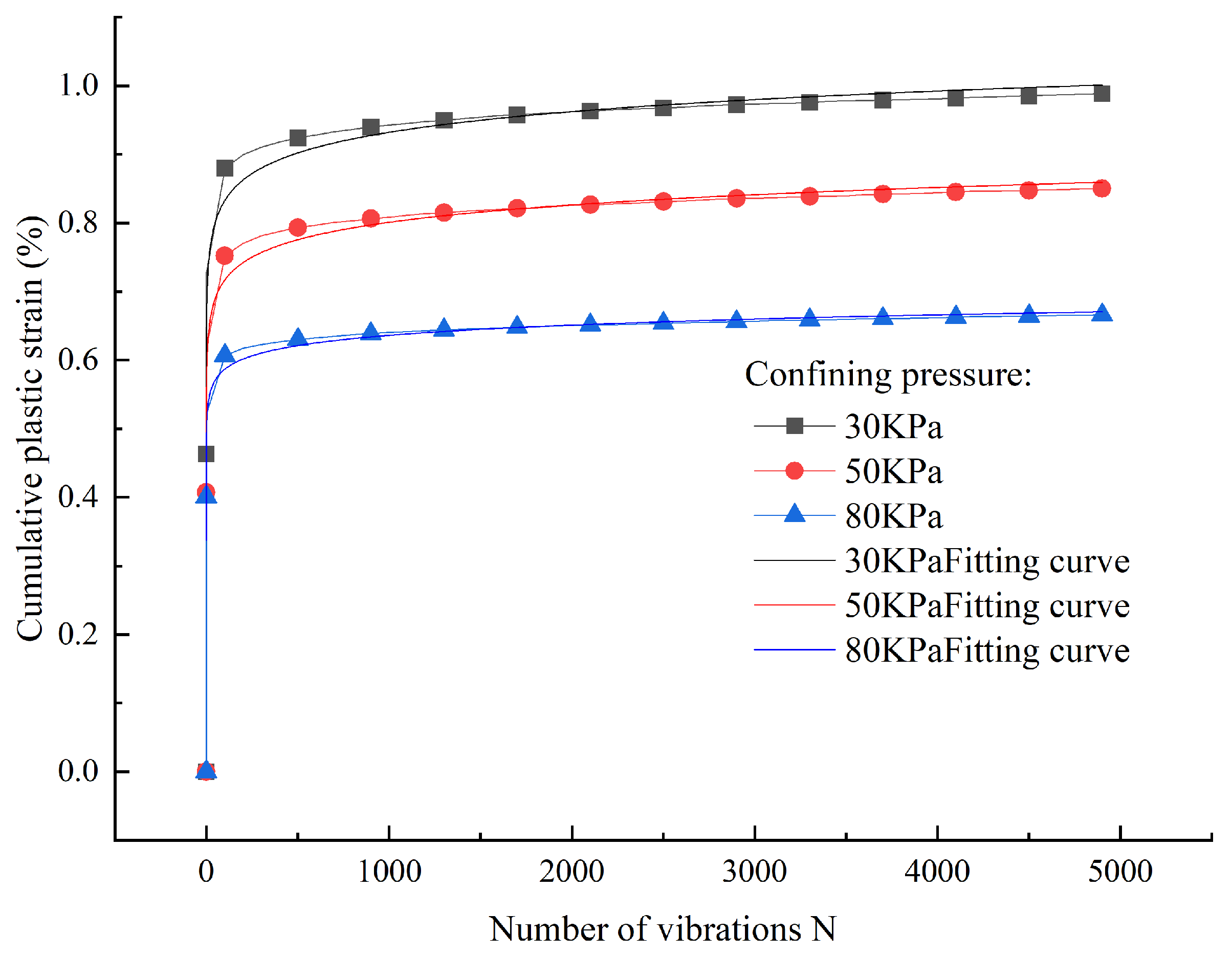
3.3. Fitting Relationship Between Dynamic Elastic Modulus and Dynamic Strain

Experimental data were obtained using a GDS dynamic triaxial apparatus (GDSLAB2.6.6), and the variation of dynamic elastic modulus with dynamic strain amplitude under different confining pressures, moisture contents, and frequencies was analyzed. It was found that the dynamic elastic modulus of alluvial silty sand under different conditions decreased with the increase in cumulative deformation under vibration until it tended to stabilize. At the beginning of dynamic load vibration, the dynamic elastic modulus decreased rapidly, and with the continuous accumulation of vibration times, the frequency of the dynamic elastic modulus decrease tended to 0. According to the image digital model, the non-linear least squares method is used to fit the dynamic elastic modulus strain curve as follows:

$$E_d=A{ \epsilon }^B d$$

(4)

In the formula, A and B are the material constitutive parameters obtained by fitting the experimental data, and the parameters and R² obtained under different experimental conditions are shown in

Table 4. Fitted parameters of dynamic elastic modulus for alluvial silty sand.

No.	Confining Pressure (kPa)	Moisture Content	Loading Frequency	A	B	R2
1	30	6%	1	71.975	−0.22487	0.98843
2	50	6%	1	104.486	−0.2296	0.97314
3	80	6%	1	134.70	−0.21617	0.98643
4	30	8%	1	105.3363	−0.22637	0.95928
5	30	10%	1	62.37651	−0.25859	0.97944
6	30	8%	3	105.678	−0.22638	0.95936
7	30	8%	5	101.10384	−0.23329	0.96086

. Keeping the moisture content and loading frequency constant, the curve fitting method of Formula (4) was used to obtain the dynamic elastic modulus–dynamic strain fitting curves under various confining pressures, as shown in Figure 6. The analysis shows that the R² values under different test conditions are all greater than 0.95, and the visual verification of the curve in Figure 6 confirms that the fit obtained is relatively reliable.

4. Finite Element Analysis

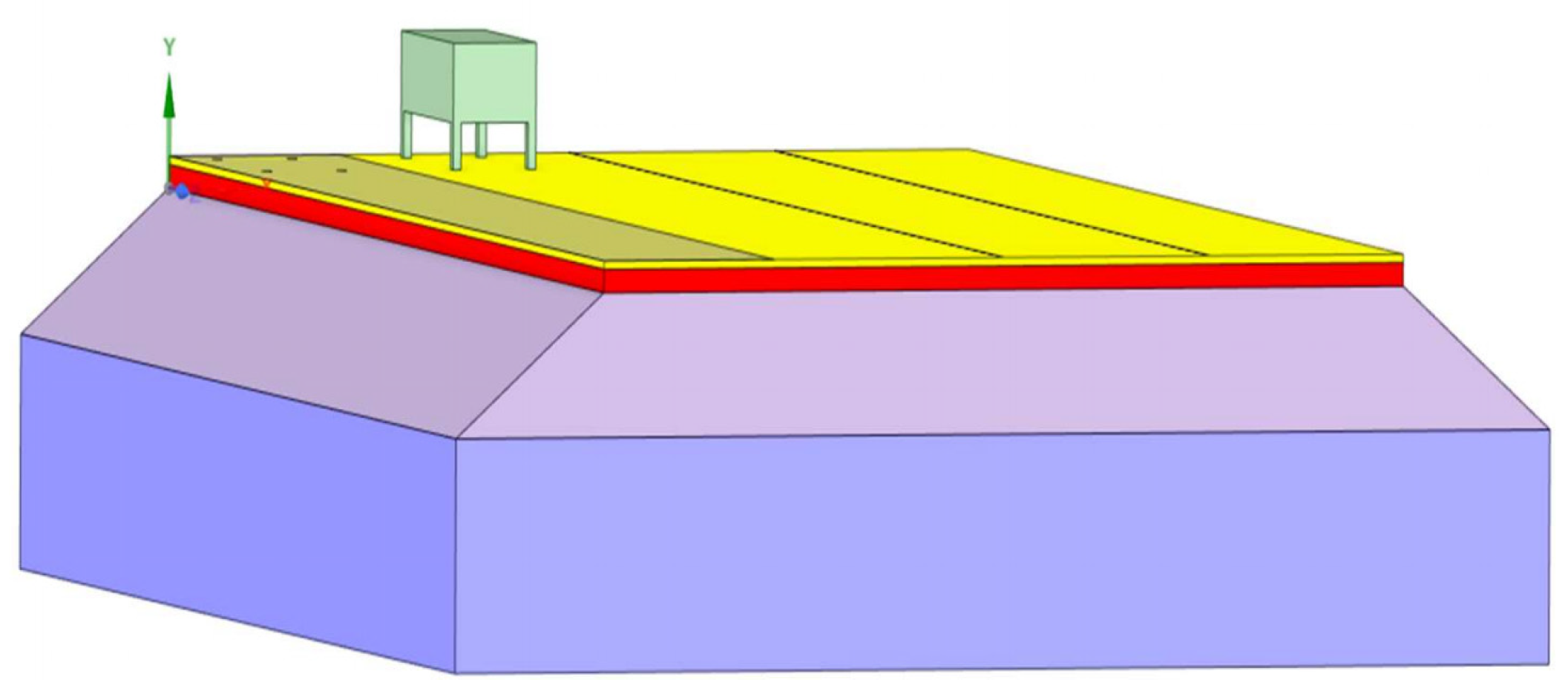
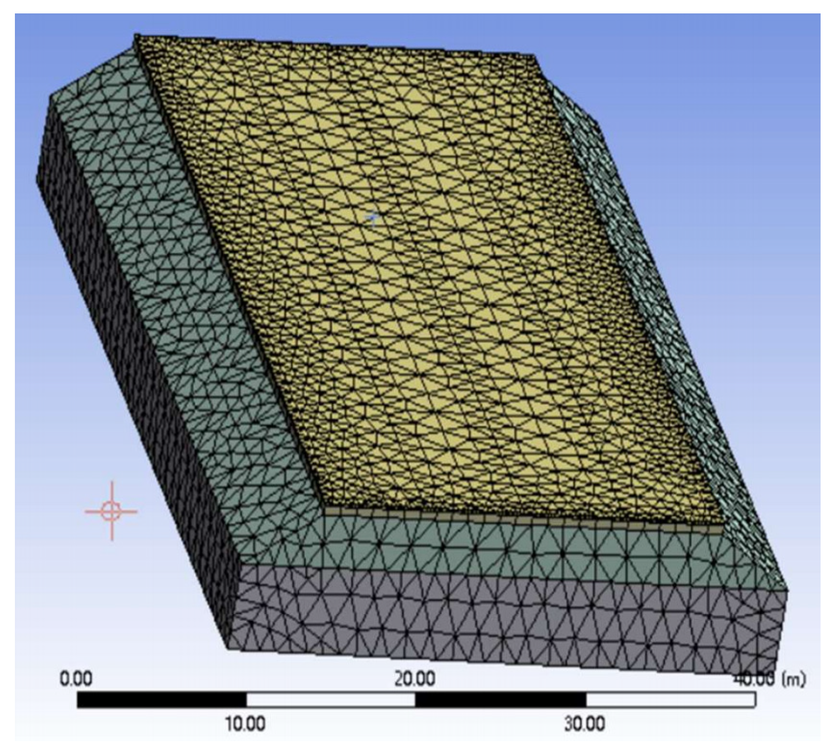
4.1. Model Determination

Based on the cross-section of the K49 + 534.7 section of the Chicao Expressway, a finite element model was constructed using ANSYS 2020R2 (Figure 7). In this model, the surface layer thickness is set to 0.18 m, the base layer thickness is 0.56 m, the roadbed soil layer thickness is 3 m, and the underlying foundation soil layer thickness is 5 m. In the xoy coordinate system, the road structure is 25.24 m wide and the upper and lower surface lengths of the roadbed are 25.24 m and 30 m, respectively, forming a slope ratio of 1:1.5. The model has spring damper boundaries on both sides, a completely fixed bottom boundary, and a top boundary representing a free surface with load pressure.

To simulate the dynamic load effect, a sinusoidal pressure is applied, and its expression is p(t) = k₁b₁ sin(ωt + θ) + p₀. This formula accurately describes the harmonic vibration of the vehicle suspension system, and after comprehensive consideration, the maximum value of dynamic stress amplitude of 40 kPa is selected. Due to the high strength of the pavement structure, it is modeled as an elastic body; the roadbed and foundation are considered elastic–plastic bodies. The elastic part is described using a linear elastic model, while the elastic–plastic part is characterized using a Mohr Coulomb model. In addition, for the convenience of calculation and to improve accuracy, equivalent viscoelastic boundary conditions were implemented in the boundary region: artificial boundaries containing viscous damping (energy dissipation) and elastic restoring force (stiffness simulation) were applied to the lateral and bottom boundaries of the finite element model to simulate unrestricted soil and suppress wave reflection.

In the computational model of this study, the pavement structure design considers the case of two lanes where vehicle loads are concentrated on the central lane. The interaction area between the wheels and the ground is idealized as a rectangle, with a size of 0.24 m × 0.3 m, which corresponds to the typical grounding imprint of a standard double wheel set with an axle load of 100 kN (tire pressure of 0.7 MPa). The pressure-sensitive membrane test in reference [27] has verified its effectiveness. This simplification optimizes grid density while preserving the true stress distribution. The finite element mesh division is shown in Figure 8, using hexagonal and quadrilateral elements to accurately capture the structural response characteristics.

Select hexagonal and quadrilateral elements to adapt to the geometric characteristics of embankment slopes while ensuring accuracy. Grid sensitivity analysis shows that the key output results (stress/displacement) differ by less than 2% compared to 8-node brick elements.

4.2. Simulation Conditions

When conducting model calculations, the basic parameters of the pavement base and surface layers are determined through methods such as unconfined compressive tests, standard specifications, the ring knife method, and direct reference to the literature, as shown in

Table 5. Structural layer parameters.

Layer	Parameter
	Elastic Modulus (MPa)	Poisson’s Ratio	Density (kg/m3)	Cohesion (kPa)	Internal Friction Angle	Damping Ratio
Surface Layer	1200	0.25	2300	-	-	0.12
Base Layer	1500	0.25	2200	-	-	0.1
Subgrade	120	0.32	2120	22.4	32.5	0.15
Foundation	38	0.35	1600	27.6	28.4	0.2

. For the cohesion and internal friction angle, indoor direct shear tests were used for measurement, and on-site cross-plate shear tests were used for verification. Consider the effects of vehicle speed, moisture content, and compaction degree and analyze various conditions. The selection of vehicle speed covers the typical operating range of heavy-duty trucks, the moisture content includes the optimal value (7.8%) and the measured extreme value on site, and the selection of compaction degree complies with the construction specifications (JTG D30-2015 [34]). In addition, the constant modulus assumption is only used for comparative analysis. Listed in

Table 6. Simulation conditions.

Driving Speed (km/h)	Moisture Content (%)	Base Layer Modulus (MPa)	Base Layer Thickness (cm)	Compaction Degree (%)
30, 60, 80, 90	8	1300	56	96
	8, 10	1500	56, 64, 72	96
	8	1700	56	96

.

4.3. Model Validation

By comparing the finite element simulation results with the on-site monitoring data of the H1 section (K49 + 347.5) of the Chicao Expressway, the results show that the model has high reliability. The maximum settlement calculated by simulation is 14.2 mm, with only a deviation of 1.25% compared to the measured maximum value of 14.38 mm. In terms of settlement patterns, both simulated and measured data exhibit a typical bowl-shaped distribution characteristic of “large in the middle and small on the shoulder”, with a settlement deviation of less than 5% in the shoulder area. In terms of stable time, the 24-day stable period predicted by simulation is highly consistent with the 22–26-day stable range observed on site. In addition, the coefficient of determination (R²) between simulated and measured dynamic stresses reached 0.91, showing a good correlation, with only a difference of less than 3% in shallow stresses, mainly due to the microscopic non-uniformity of on-site compaction. These comparative results fully validate the accuracy and applicability of the established finite element model.

5. Analysis of Engineering Characteristics Results

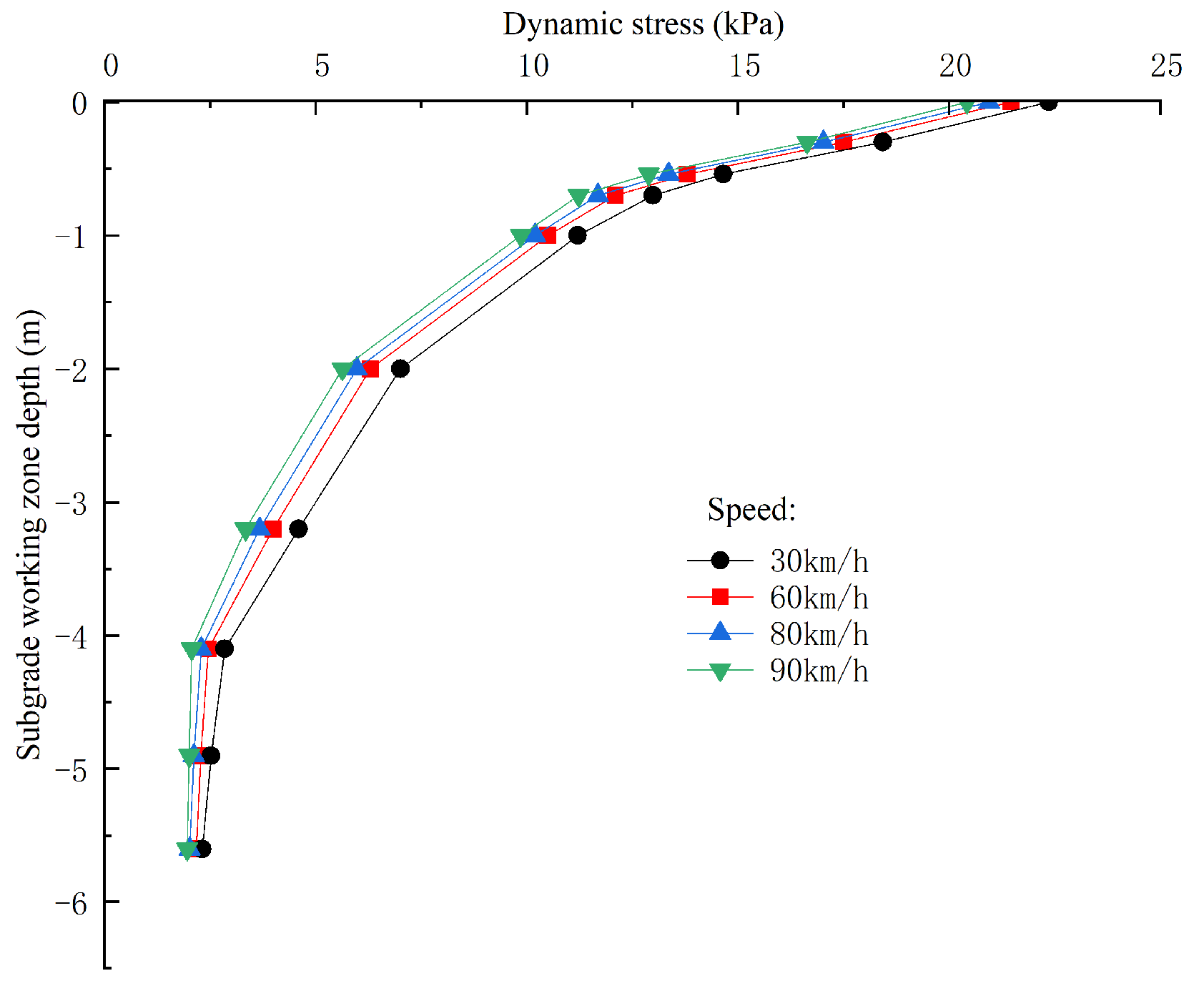
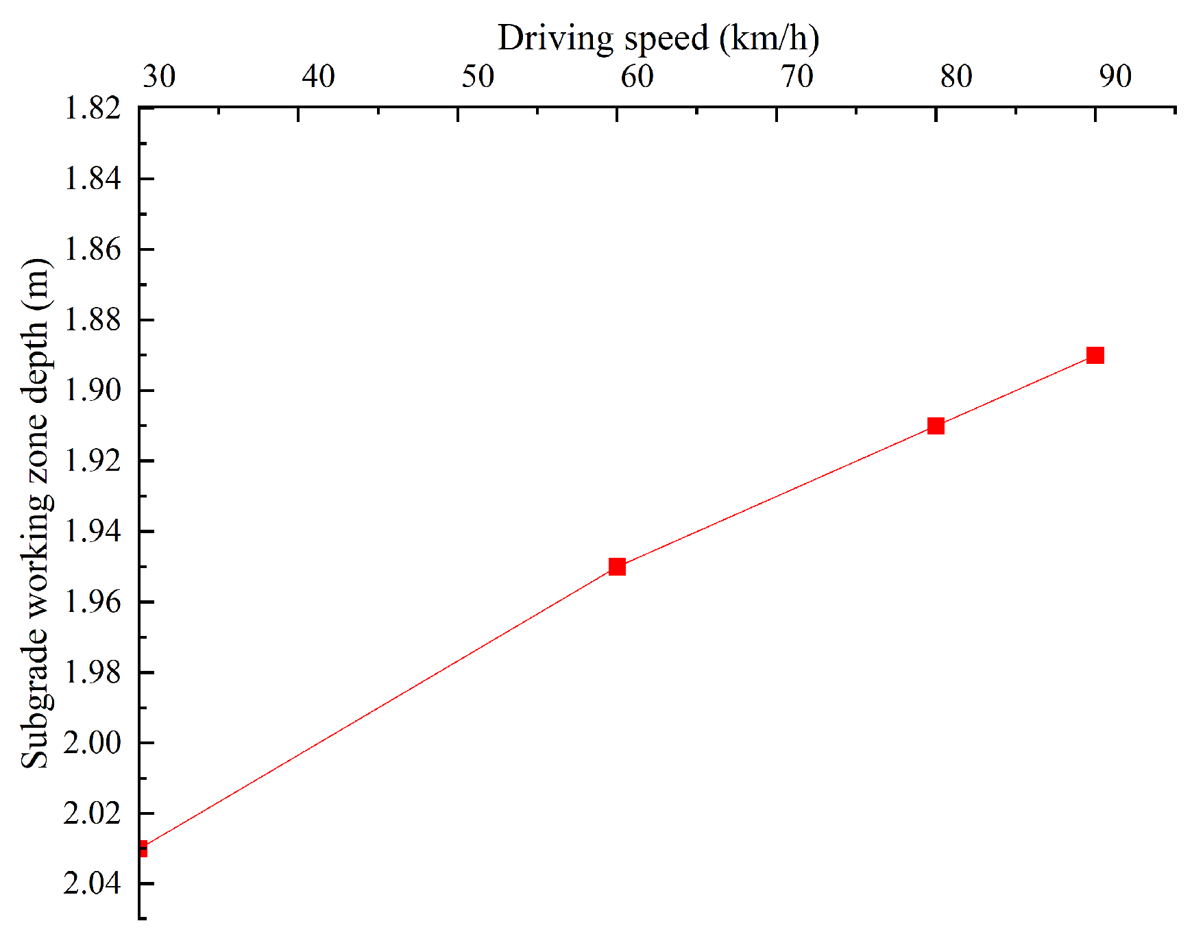
5.1. Influence of Speed

The speed of a vehicle affects its dynamic stress on the road surface, which is manifested in the duration of contact between the vehicle and the road surface. The shorter the contact time, the faster the vehicle speed. The test results are shown in

Table 7. Dynamic stress variation range corresponding to different driving speeds.

Driving Speed (km/h)	Dynamic Stress Variation Range (kPa)
30	2.32~22.64
60	2.13~21.38
80	2.02~20.95
90	1.96~20.42

, where the stress range is the 90% confidence interval of 100 simulated load cycles at each vehicle speed. By combining finite element analysis with on-site measured data, the relationship between dynamic stress and depth at different vehicle speeds was obtained, as shown in Figure 9. The finite element simulation average of 50 load cycles at each vehicle speed was obtained to determine the relationship between dynamic stress and driving speed at different depths, as shown in Figure 10. Simulate the dynamic stress distribution at different depths under four different vehicle speeds, and obtain the attenuation law of dynamic stress with roadbed depth under different vehicle speeds, as shown in Figure 11.

Based on Figure 9 and Figure 10 and Table 7, when the vehicle moves at a constant speed, the dynamic stress gradually decreases with increasing subgrade depth. As the driving speed increases, the dynamic stress decreases to varying degrees, with reductions of 6.2% and 5.2% observed at the surface and within 6 m below the surface, respectively. Figure 11 shows that as the driving speed increases, the depth of the affected subgrade region slightly decreases, but this change is not significant. Thus, under high-speed conditions (90 km/h), due to the shallow impact depth, the roadbed thickness can be reduced, and the drainage layer can be strengthened to guide actual engineering.

5.2. Influence of Moisture Content and Compaction Degree

5.2.1. Moisture Content

Control the moisture content parameters at 8% and 10%, representing the typical allowable range for roadbed compaction. In practical engineering, if the soil is too dry or too wet, it can be treated by watering and adding 3–5% quicklime. The corresponding shear strengths obtained from the triaxial tests were 22.4 kPa, 32.5° and 18.7 kPa, 33.4°, respectively. A standard driving speed of 60 km/h was applied, while the other parameters remained constant. Figure 12 and Figure 13 illustrate the variation of dynamic stress with depth and the displacement changes along the driving lane direction under different moisture content conditions under simulated vehicle loading.

Table 8. Dynamic stress range by moisture content.

Moisture Content (%)	Dynamic Stress Variation Range (kPa)
8	2.63~24.62
10	2.54~22.35

presents the dynamic stress within 6 m below the subgrade surface under different moisture content conditions.

According to Figure 12 and Table 8, the dynamic stress decreases with increasing subgrade depth. For moisture contents of 8% and 10%, the dynamic stress decreases by 92.3% and 96.9%, respectively, from the surface to the bottom. At the load application point, the maximum dynamic stress occurs, with a difference of 2.1% between the 8% and 10% moisture content conditions. Figure 13 shows that the maximum vertical displacement is located at the top of the roadbed. As the moisture content increases, the cohesive force of the alluvial silt decreases. When the moisture content increases from 8% to 10%, the maximum displacement at the top increases by 104.8%. This is because the dynamic load under wetter conditions will produce significantly higher pore water pressure, reduce effective confining pressure, and accelerate deformation. This indicates that a high moisture content has a significant impact on the mechanical behavior of shallow areas. Although the optimal moisture content (7.8%) is close to the plastic limit (8.4%), on-site data show that the roadbed is stable when the compaction degree is greater than 94%. After construction, it is necessary to monitor the moisture content to prevent it from exceeding the plastic limit in order to avoid a decrease in strength.

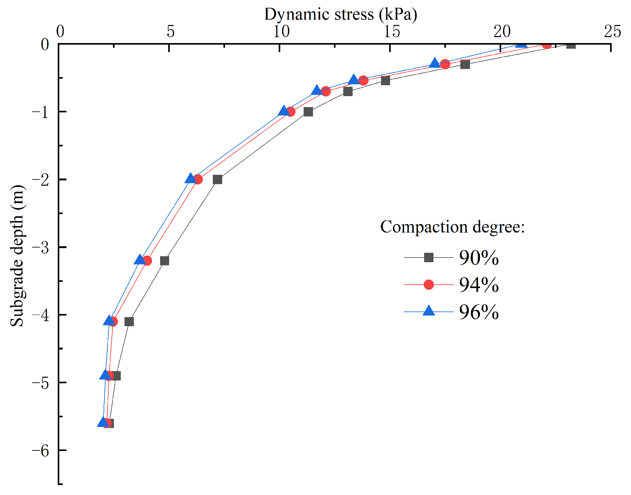
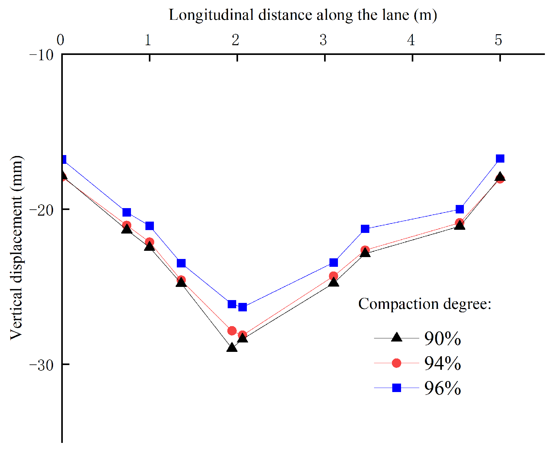
5.2.2. Compaction Degree

In the finite element analysis model, three different compaction degrees were set—90%, 94%, and 96%—while maintaining a load moving speed of 60 km/h and a fixed moisture content of 8%. The other parameters remained consistent. In practical engineering, three-stage control can be adopted, with detection frequencies of 50 m and 20 m, and continuous monitoring. Figure 14 and Figure 15 illustrate the variation of dynamic stress with depth and the displacement changes along the driving lane direction under different compaction degrees under simulated vehicle loading. The results were obtained through dynamic finite element simulation based on the loading conditions described in Section 3.1.

Table 9. Dynamic stress range by compaction degree.

Compaction Degree (%)	Dynamic Stress Variation Range (kPa)
90	2.33~23.62
94	2.18~22.13
96	2.02~20.95

presents the dynamic stress within 6 m below the subgrade surface under different compaction degrees.

According to the data in Figure 14, the dynamic stress gradually decreases with increasing vertical depth of the subgrade, and the rate of decrease slows down. Under different compaction degrees, the dynamic stress from the subgrade surface to the bottom decreases by 93.6% (90% compaction), 94.7% (94% compaction), and 94.3% (96% compaction), respectively. Figure 15 shows that the maximum vertical displacement occurs at the center of the load application point. When the compaction degree decreases from 96% to 90%, the maximum settlement at the subgrade surface increases from 20.95 mm to 23.62 mm, representing an increase of 10.4%. This indicates that increasing the compaction degree beyond 90% has a limited effect on reducing settlement.

6. Field Monitoring

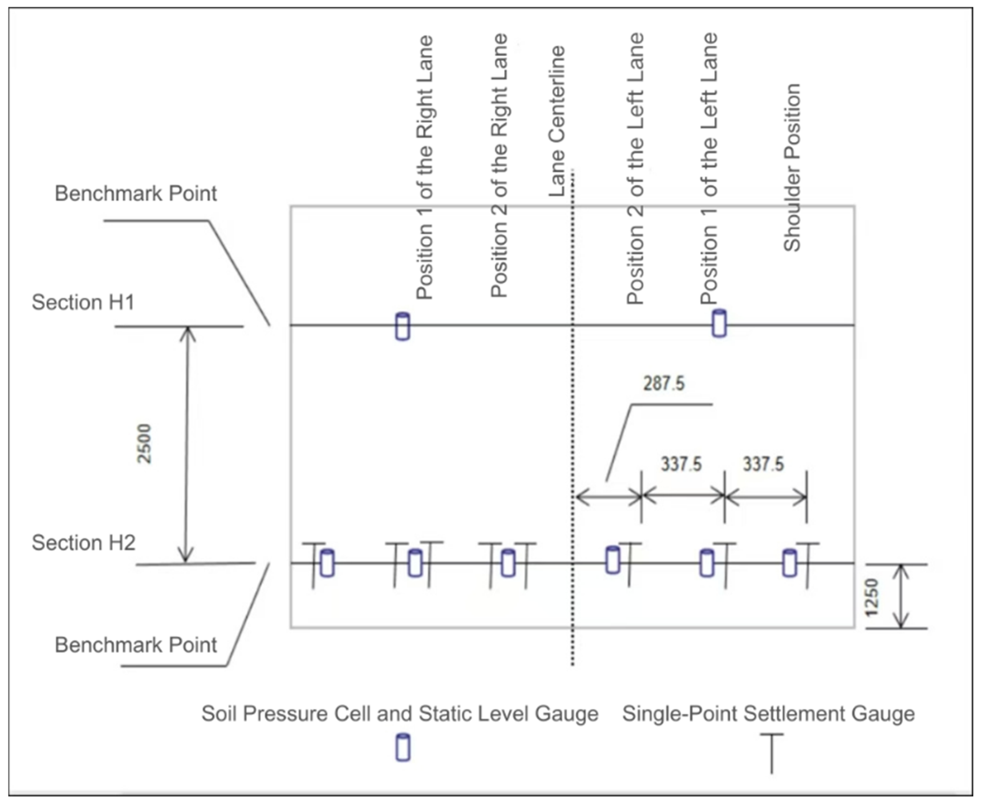
6.1. Instrument Selection and Principles

For the H1 section (at K49 + 347.5) and the H2 section (at K49 + 372.5) of the Chicao Expressway, settlement and pressure changes were observed and analyzed comparatively. Field monitoring was conducted using single-point settlement gauges to measure the absolute settlement at specific points within the subgrade, static level gauges to assess uneven settlement across the subgrade cross-section, and earth pressure cells to monitor the conditions at the bottom of the stabilized soil layer. The layout of the monitoring equipment is shown in Figure 16.

The static level is commercially available standard equipment with a range of ±50 mm and an accuracy of ±0.1 mm. It includes multiple storage tanks and sensors. The sensors are pre-embedded during roadbed construction according to the “Technical Specification for Highway Roadbed Monitoring” (JTG/T D31-02-2023 [37]) and connect to the storage tanks through a filling pipeline to measure liquid level changes caused by settlement. During burial, the storage tank and monitoring points remain in a horizontal position and stay relatively stable. Under automobile load, when the monitoring points in the roadbed sink, the liquid in the storage tank changes, and the sensors detect the roadbed settlement.

The single-point settlement gauge measures soil deformation and displacement. It consists of displacement meters, flange settlement plates, and other components. Its advantage is automatic monitoring and long-term use, making it suitable for measuring soil deformation between anchor heads and settlement plates. During use, the anchor end fixes to a relatively stable point, and the buried elevation of the settlement plate requires detection. A data line extends from the side. When the foundation sinks, the settlement plate drives the magnet in the sensor to displace, allowing the relative displacement to be read.

The earth pressure cell is a steel string sensor that measures internal soil stress. Its range is 0–500 kPa, accuracy is ±0.5% FS, and resolution is 0.1 kPa. It can be pre-embedded before roadbed construction or installed by drilling afterward. This sensor measures the pressure distribution in roadbeds and soil pressure changes under dynamic loads, and monitors the stability of road cut slopes.

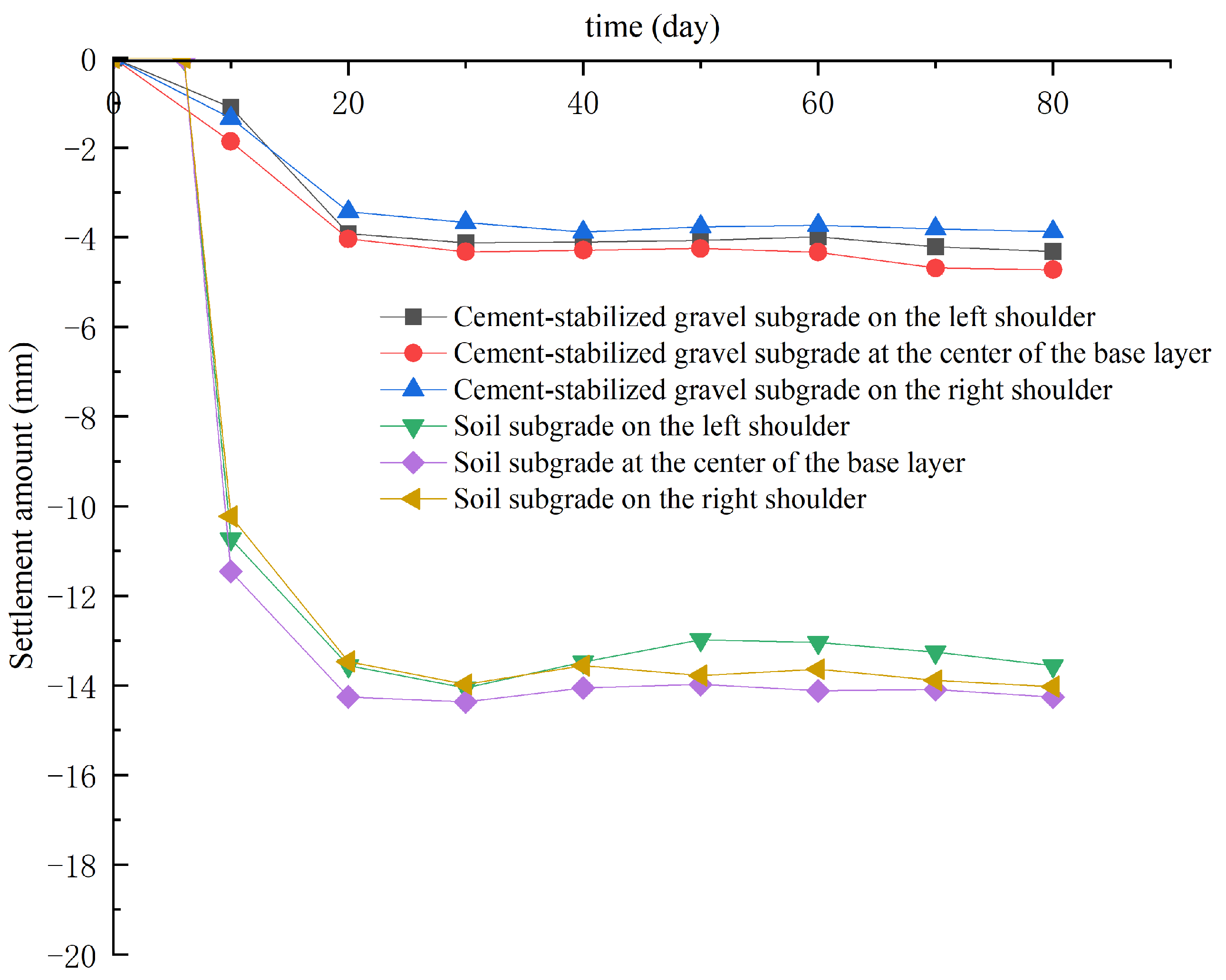
6.2. Results Analysis

A comparative observation was conducted using cement-stabilized gravel and alluvial silty sand as the upper materials of the subgrade cushion layer. The settlement of the embankment surface during construction was measured, as shown in Figure 17:

The results show that the maximum compression settlement of the alluvial silty sand filler occurs at the center, measuring 14.38 mm, with settlements of 13.84 mm and 14.20 mm at the left and right shoulders, respectively, indicating a larger settlement in the middle and smaller settlements on the sides. When cement-stabilized gravel is used as the filler, the settlement is significantly reduced, with the center settlement at 4.64 mm and the left and right shoulder settlements at 3.56 mm and 3.98 mm, respectively. These observations reflect the compression and consolidation process of the fill materials.

Excluding the influence of the foundation and cushion layers, when alluvial silty sand is used as the filler, the subgrade settlement stabilizes within approximately 24 days, with settlement values ranging between 12 and 14 mm. When cement-stabilized gravel is used as the filler, the settlement stabilizes within about 21 days, with settlement values controlled between 3 and 5 mm.

A comparison of subgrade settlement under these two fill conditions reveals that although the alluvial silty sand filler exhibits a larger settlement magnitude and rate, it does not significantly affect the overall stability of the subgrade. This indicates that despite its higher initial settlement characteristics, alluvial silty sand can still meet engineering requirements in terms of long-term performance. Therefore, alluvial silty sand can replace cement gravel for non-critical road sections to save material costs. Xu et al. [27], through their research on the life cycle carbon emissions of ecological slope protection, pointed out that selecting environmentally friendly materials during the construction and maintenance phases can significantly reduce carbon emissions. This finding aligns closely with the potential of alluvial silty sand as a sustainable filler material.

7. Conclusions

This article, for the first time, systematically studies the roadbed engineering characteristics of alluvial silty sand under traffic loads through the integration of theoretical analysis, finite element simulation, and on-site detection methods. The main conclusions are as follows:

(1)

The change in vehicle speed has a relatively small effect on the distribution and depth of dynamic stress. Under high-speed conditions (such as 90 km/h), dynamic stress attenuation is faster and the impact depth is shallower. Therefore, the design of roadbed thickness can be appropriately optimized and drainage measures can be strengthened to improve the economic efficiency of the project.

(2)

Moisture content and compaction degree are key factors affecting the performance of alluvial silty sand subgrade. Research has shown that an increase in soil moisture content can lead to a decrease in its shear strength, an increase in dynamic stress, and a significant increase in displacement at the top of the roadbed (for example, when it increases from 8% to 10%, the displacement at the top increases by 104.8%). Improving compaction can help reduce roadbed settlement and enhance the overall stability and safety of the roadbed.

(3)

The finite element simulation results are in good agreement with the on-site monitoring data, verifying the reliability of the model and providing an effective analysis tool for similar projects. However, the assumption of the homogeneous subgrade used in the model may to some extent underestimate the impact of actual soil layer stratification effects.

(4)

The initial settlement of alluvial silty sand filling is relatively large, but the settlement rate is fast and can stabilize within 24 days, and its long-term performance meets the engineering requirements. Compared with cement crushed stone filling, although its settlement is significantly increased, it has no significant impact on overall stability and can be used as an economic alternative material for non-critical road sections. Xu et al. [28], based on life cycle theory and the Sobol method, further analyzed the carbon emissions of ecological slope protection. Their results indicate that the rational selection of filler materials can significantly reduce the environmental impact of engineering projects. This provides theoretical support for the application of alluvial silty sand in the field of environmental protection.

(5)

The use of alluvial silty sand as roadbed filling material is feasible, but it is necessary to strictly control the moisture content and compaction degree during construction, and strengthen drainage design. Its environmental and economic benefits further support its potential application in sustainable engineering. It is suggested that future research be conducted to test the performance of alluvial silt under different geological conditions (such as coastal or mountainous areas), analyze the influence of factors such as salinity or geological structure, and make the results applicable to more engineering scenarios.

References

1. Jiang, L. Model Experimental Study on Mechanical Characteristics of Support Structures for Highway Tunnels in Granite Residual Soil. J. Hunan Univ. Arts Sci. (Nat. Sci. Ed.) 2023, 35, 76–80. [Google Scholar]
2. Sun, J. Some Advances in Rock Rheological Mechanics and Its Engineering Applications. Chin. J. Rock Mech. Eng. 2007, 26, 1081–1106. [Google Scholar]
3. Wang, X. Experimental Study on Engineering Mechanical Properties of Silty Soil Deposited by the Yellow River in the Yellow River Floodplain. Build. Technol. Dev. 2022, 49, 114–116. [Google Scholar]
4. Long, J. Application of Cement Mixing Piles in Soft Soil Foundation Construction of Municipal Roads. Sichuan Build. Mater. 2022, 48, 186–187, 224. [Google Scholar]
5. Min, J.; Zou, Y. Application of foam lightweight soil in rapid reconstruction of urban roads. Urban Roads Bridges Flood Control 2022, 12, 233–235+28. [Google Scholar] [CrossRef]
6. Deng, T.; Ma, B.; Zou, Y.; Wang, Q.; Song, C. Influence of sample preparation methods on road performance indicators of red clay. Subgrade Eng. 2022, 6, 90–95. [Google Scholar] [CrossRef]
7. Wang, X.; Yang, J. Physical and Mechanical Properties of Red Sandstone and Its Compaction Energy for Subgrade Construction. J. Zhejiang Univ. Sci. Technol. 2022, 34, 551–558. [Google Scholar]
8. Wang, C. Study on Mechanical Properties of Cement-Modified Sedimentary Silty Sand Roadbed. Highway 2023, 68, 75–79. [Google Scholar]
9. Xu, J.; Zhao, D.; Wang, S.; Chen, X.; Wu, X.; Han, Z.; Liu, Y. Quantitative analysis of pore structure’s impact on early mechanical properties and durability of foam concrete: Macroscopic and mesoscopic insights. Constr. Build. Mater. 2025, 459, 139775. [Google Scholar] [CrossRef]
10. Wang, X.; Zhang, J.; Yang, G.; Chen, X. Dynamic stress testing of highway subgrade and base layer under heavy loads. J. Vib. Shock 2007, 26, 169–173. [Google Scholar]
11. Wang, X. Study on Dynamic Response of Flexible Pavement Structure and Subgrade Under Random Loads. Ph.D. Thesis, Central South University, Changsha, China, 2006. [Google Scholar]
12. Jiang, Y.; Li, S.; Wang, T. Numerical method of dynamic triaxial test on graded crushed rock. J. Southeast Univ. (Nat. Sci. Ed.) 2013, 43, 604–609. [Google Scholar]
13. Ni, X.; Ye, B. Unit test and simulation of liquid-solid phase transition mechanism after sand liquefaction. J. Tongji Univ. (Nat. Sci. Ed.) 2023, 51, 16–22. [Google Scholar]
14. Lou, Q.; Tao, T.; Tian, X.; Xie, C. Numerical simulation method for impact failure patterns of limestone based on HJC constitutive model. Blasting 2022, 39, 71–79. [Google Scholar]
15. Weng, L.; Zhang, H.; Zhang, Y.; Chu, Z.; Xu, X. Dynamic mechanical properties and constitutive model of water-saturated siltstone under low temperature. Chin. J. Appl. Mech. 2022, 39, 1096–1107, 1134. [Google Scholar]
16. Sun, D.; Wu, B. Study on dynamic elastic modulus and damping ratio of unsaturated silt. J. Hydraul. Eng. 2012, 43, 1108–1113, 1120. [Google Scholar]
17. Chen, G.; Wang, B.; Liu, J. Experimental study on dynamic shear modulus and damping ratio of recently deposited soils. J. Undergr. Space Eng. 2008, 4, 539–543, 594. [Google Scholar]
18. Xie, Y.; Chen, T.; Wang, J.; Gu, S.; Zhu, F. Dynamic shear characteristics of frozen clay-concrete interface. J. Railw. Sci. Eng. 2022, 19, 2637–2646. [Google Scholar]
19. Tang, Y.; Wang, Y.; Huang, Y.; Zhou, Z. Dynamic strength and dynamic stress-strain relationship of soil under subway traffic loads. J. Tongji Univ. (Nat. Sci. Ed.) 2004, 32, 701–704. [Google Scholar]
20. Chen, Y.; Huang, B.; Chen, Y. Deformation and strength characteristics of structured soft clay under cyclic loading. Chin. J. Geotech. Eng. 2005, 27, 1065–1071. [Google Scholar]
21. Chen, S. Study on Engineering Characteristics and Treatment Techniques of Expansive Soil. Doctoral Dissertation, Huazhong University of Science and Technology, Wuhan, China, 2006. [Google Scholar]
22. Dai, S.; Van Deusen, D. Field study of in situ subgrade soil response under flexible pavements. Transp. Res. Rec. 1998, 1639, 23–35. [Google Scholar] [CrossRef]
23. Zhu, Z.; Wang, Y.; Gong, W.; Feng, Q. Dynamic Analysis Method for Vehicle-Track Vertical Coupling System Based on Transfer Matrix Method. J. Vib. Shock 2022, 41, 31–38. [Google Scholar]
24. Sun, J.; Li, M.; Tian, H. Dynamic Load Response Analysis of Heavy-Duty Vehicles on Uneven Road Surfaces. J. Chongqing Jiaotong Univ. (Nat. Sci. Ed.) 2019, 38, 48–53. [Google Scholar]
25. Xu, L.; Guo, W.; Wang, J.; Fang, C.; Zhang, Z. Performance of recycled aggregate concrete based on a new classification method. Constr. Build. Mater. 2016, 101, 469–477. [Google Scholar]
26. Dai, G.; Huang, M.; Xu, Q.; Qiu, Y. Dynamic response of saturated porous media under cyclic loading. Soil Dyn. Earthq. Eng. 2018, 113, 1–11. [Google Scholar]
27. Xu, J.; Wu, X.; Qiao, W.; Wang, S.; Shu, S.; Zhao, D.; Chen, X. Life cycle carbon emission assessment for ecological protection slopes: Focus on construction and maintenance phases. J. Clean. Prod. 2025, 497, 145174. [Google Scholar] [CrossRef]
28. Xu, J.B.; Wu, X.; Qiao, W.; Wang, S.; Chen, X.; Zhao, D.; Zeng, X.; Shu, S. Carbon emission analysis of ecological slope protection based on lifecycle theory and sobol method. Ecol. Eng. 2025, 215, 107584. [Google Scholar] [CrossRef]
29. ASTM D2487-17; Standard Practice for Classification of Soils for Engineering Purposes (Unified Soil Classification System). ASTM International: West Conshohocken, PA, USA, 2017.
30. GB/T 50145-2007; Standard for Engineering Classification of Soils. Ministry of Housing and Urban-Rural Development of the People’s Republic of China: Beijing, China, 2007.
31. ASTM D6913/D6913M-17; Standard Test Methods for Particle-Size Distribution (Gradation) of Soils Using Sieve Analysis. ASTM International: West Conshohocken, PA, USA, 2017.
32. ASTM D4318-17; Standard Test Methods for Liquid Limit, Plastic Limit, and Plasticity Index of Soils. ASTM International: West Conshohocken, PA, USA, 2017.
33. ASTM D698-12; Standard Test Methods for Laboratory Compaction Characteristics of Soil Using Standard Effort (12,400 ft-lbf/ft3 (600 kN-m/m3)). ASTM International: West Conshohocken, PA, USA, 2012.
34. JTG D30-2015; Specifications for Design of Highway Subgrades. Ministry of Transport of the People’s Republic of China: Beijing, China, 2015.
35. Guo, G.; Ding, W.; Zhang, C. Analysis of stochastic dynamic load acting on rough road by heavy-duty traffic. In Proceedings of the 12th International Conference of Chinese Transportation Professionals (CICTP 2012): Multimodal Transportation Systems—Convenient, Safe, Cost-Effective, Efficient; American Society of Civil Engineers (ASCE): Reston, VA, USA, 2012; pp. 3194–3205. [Google Scholar] [CrossRef]
36. Wang, S.W.; Xu, J.B.; Wu, X.; Qi, Y.; Chen, X.; Zeng, X.; Qiao, W.; Dong, T. Creep constitutive model of coral sand. Bull. Eng. Geol. Environ. 2025, 84, 85. [Google Scholar] [CrossRef]
37. JTG/T D31-02-2023; Technical Specifications for Highway Subgrade Monitoring. Ministry of Transport of the People’s Republic of China: Beijing, China, 2023.
Figure 1. Quarter-vehicle vibration model.
Buildings 15 01375 g001
Figure 2. Particle size distribution curve.
Buildings 15 01375 g002
Figure 3. Compaction curve.
Buildings 15 01375 g003
Figure 4. GDS dynamic triaxial testing apparatus.
Buildings 15 01375 g004
Figure 5. Fitted dynamic stress–strain curve under cyclic loading.
Buildings 15 01375 g005
Figure 6. Fitted dynamic elastic modulus–strain curve.
Buildings 15 01375 g006
Figure 7. Finite element model.
Buildings 15 01375 g007
Figure 8. Mesh division.
Buildings 15 01375 g008
Figure 9. Relationship between dynamic stress and depth.
Buildings 15 01375 g009
Figure 10. Relationship between dynamic stress and moving load speed.
Buildings 15 01375 g010
Figure 11. Relationship between subgrade depth and driving speed.
Buildings 15 01375 g011
Figure 12. Dynamic stress variation curves with different moisture contents.
Buildings 15 01375 g012
Figure 13. Displacement accompanying lane direction change curve.
Buildings 15 01375 g013
Figure 14. Dynamic stress vs. depth curve.
Buildings 15 01375 g014
Figure 15. Displacement vs. lane distance curve.
Buildings 15 01375 g015
Figure 16. Equipment layout.
Buildings 15 01375 g016
Figure 17. Settlement comparison for subgrade with different fill materials.
Buildings 15 01375 g017