1. Introduction
Buildings account for over 40% of primary energy use worldwide and 24% of greenhouse gas emissions [
1]. The world’s population is growing, as is the need for buildings. Hence, the reduction of energy use and increased use of energy from renewable sources are important measures for climate change mitigation. The energy-saving potential in the building sector is massive and could yield global annual energy savings equivalent to the total energy use of buildings in the USA, UK, Russia, Germany, France, and China [
2].
With increasing demand for energy-efficient buildings, the construction industry faces the challenge of ensuring that predicted energy performance is achieved once a building is in use. There are many studies that identify a performance gap between calculated/simulated energy use and actual measured energy use once buildings are in the user phase [
3,
4,
5,
6,
7,
8,
9,
10,
11,
12,
13,
14,
15,
16,
17,
18,
19,
20]. While some studies show a very large performance gap [
5,
6,
7,
13,
19], others show a lower performance gap [
8,
10,
20]. Some studies investigate the effect of deviating boundary conditions, such as internal loads and outdoor climate [
3,
4,
11,
16,
18] and some normalise the measured energy use for some of the deviating boundary conditions with respect to outdoor climate [
8,
10]. It should be noted that studies showing a low performance gap have, to some extent, normalised measured energy use. However, none of the studies attempt to normalise measured energy use for both internal and external deviating boundary conditions [
3,
4,
5,
6,
7,
8,
9,
10,
11,
12,
13,
14,
15,
16,
17].
Root causes of performance gaps have drawn the interest of researchers [
3,
5,
6,
15,
18,
19]. These causes may be sorted and attributed differently. However, root causes may be found in all stages in the building process, including the design stage and the procurement/construction stages, as well as the operational stage.
Examples of causes in the design stage may be related to inaccurate or uncertain input data [
3,
19]. Another cause could be the incorrect use of methods or tools for calculations and simulation [
6,
15]. During the construction stage, misunderstandings and incorrect execution may cause performance failure, e.g., insufficient air tightness and insulation [
3,
15]. Finally, the conditions during the actual use of a building play an important role, where occupant behaviour is often considered as the main cause of performance gaps [
3,
11,
18,
19].
Instead of normalising measured energy use, the initial simulation model, created during the design phase, may be calibrated to reflect the as-built status and the actual operating conditions during the user phase [
19,
20,
21]. After calibration, the model may be rerun with initial operating conditions with respect to indoor temperature, operating hours, exterior climate, and occupant behaviour, etc., showing as-built verified energy performance, but with the initial operating conditions. Calibrated models may match, quite closely, with measured results [
19,
21]. In other words, it is possible to overcome a performance gap due to incorrect modelling methods or tools. However, the use of calibrated models is still under development and further work is required in order to develop a good approach [
15,
21]. Furthermore, the calibration of models requires extensive measurement, which sometimes may not be possible [
15,
21].
A normalisation method of measured energy, considering both internal and external deviating boundary conditions during the actual use of a building, may allow for a meaningful comparison and verification of energy use in buildings.
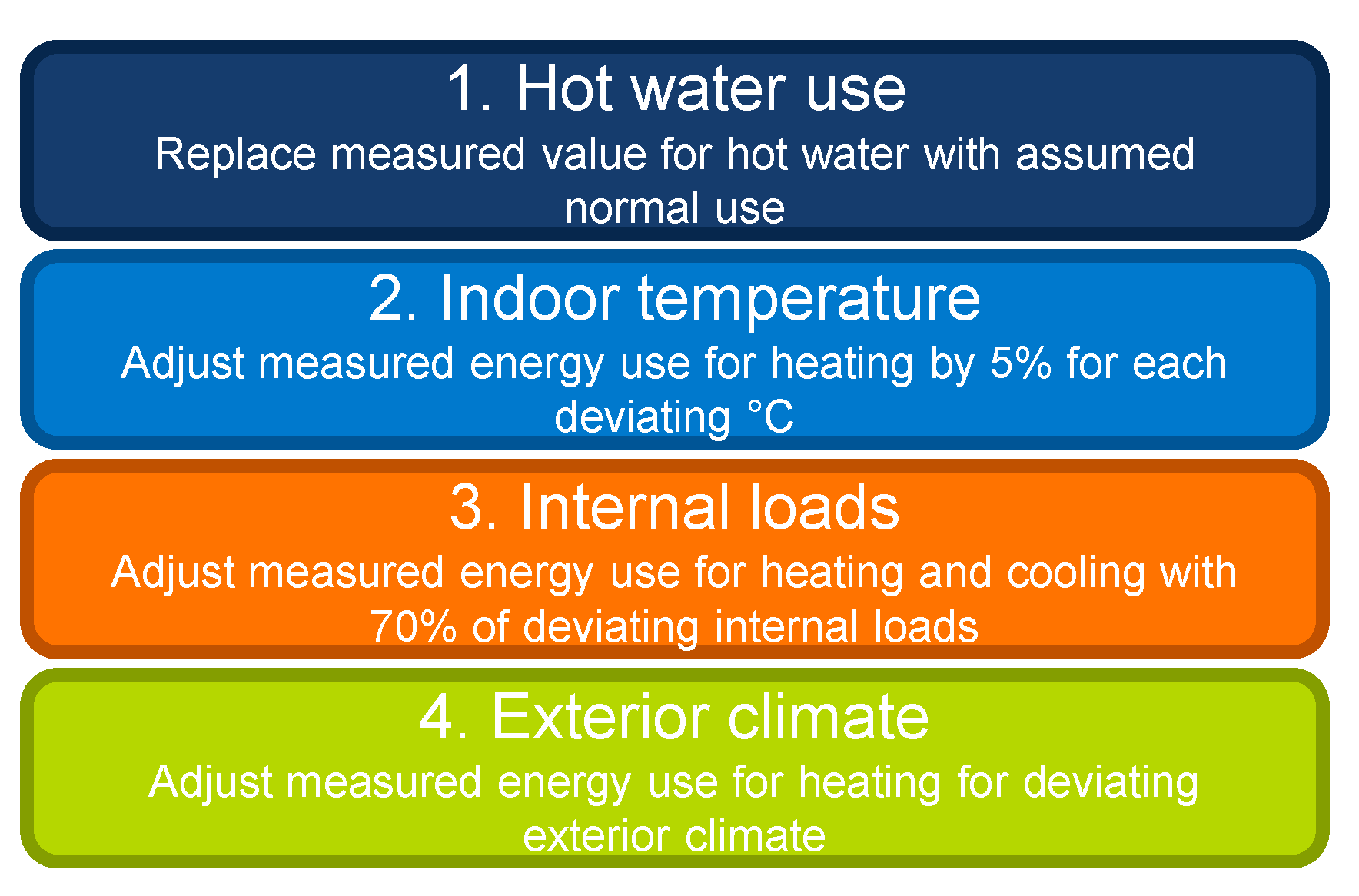
In Sweden, the National Board of Housing, Building, and Planning (Boverket) recently published a static method for normalising measured energy use, accounting for the deviation of hot water use, indoor temperature, exterior climate (outdoor temperature, solar radiation, and wind), plug loads, and lighting [
22]. In addition to this static approach, the normalisation of measured energy use is permitted, based on the relationship between the simulated energy use for normal use and for a normal year, and the simulated energy use in the case of actual use and outdoor climate during the measurement year. The second option requires dynamic simulation.
The two different methods will, in this study, be referred to as static normalisation and dynamic normalisation, respectively. Boverket stated that the methods, while simplified and shortened, are the best available methods they have been able to define. Thus, the methods are not validated.
This study presents a Net-zero energy building (Net ZEB) built in Sweden, and investigates different methods for normalising the energy use in the user phase by testing the two methods for normalising measured energy use. In this study, the Net ZEB balance is based on the Swedish regulations on energy performance [
23], which exclude energy use for plug loads and lighting. The chosen definition of a Net ZEB, used in this case, is summarised in
Table 1, and is based on the framework [
24] developed within the International Energy Agency (IEA) research project Towards Net-Zero Energy Solar Buildings [
1].
The purpose of this study is twofold; firstly, it aims to share and test the two methods for the normalisation of measured energy use in buildings, in order to enable other researchers to use, evaluate, and develop these methods. Secondly, it aims to share knowledge of building technique for a Swedish Net ZEB.
The static model from Boverket has the objective of being a simple and straightforward normalisation method, closing the performance gap due to deviating conditions during the actual use of a building, which are often considered the main cause of performance gaps [
3,
11,
18,
19].
3. Description of the Case Study
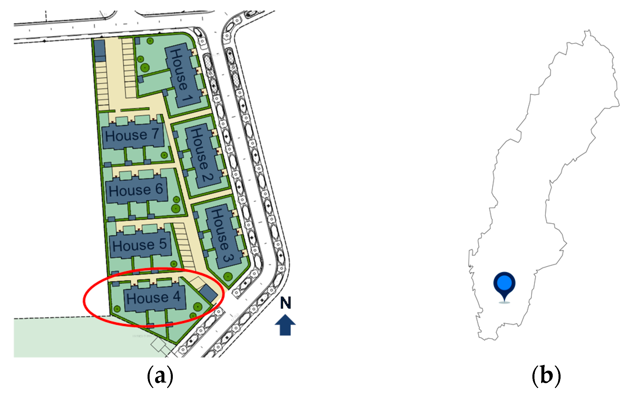
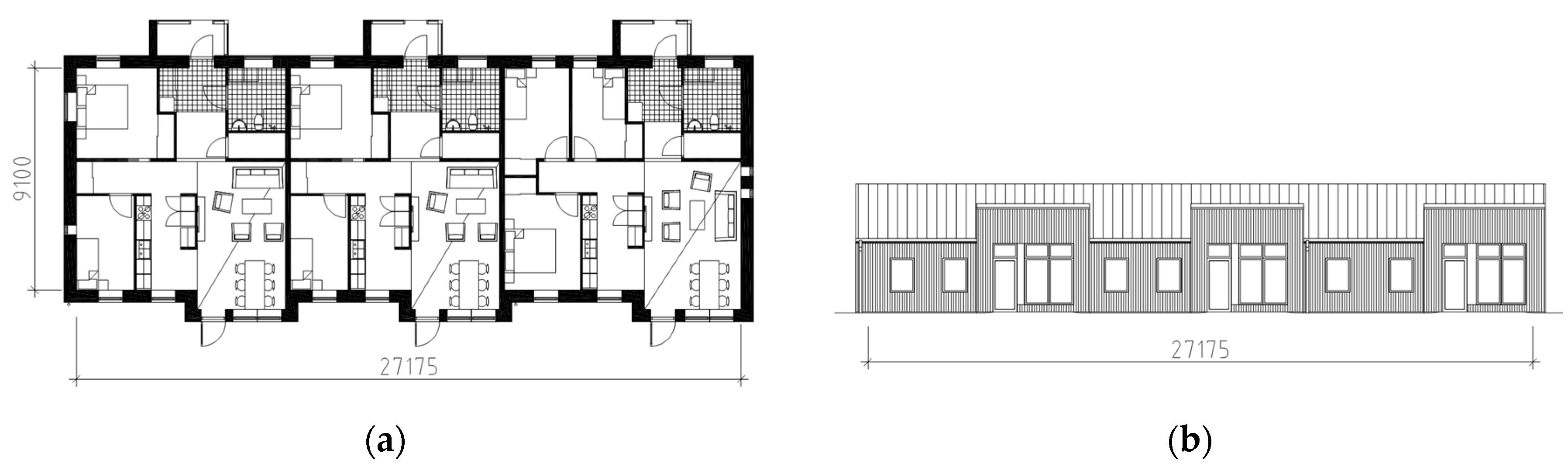
Solallén consists of 21 dwellings in seven one-storey terraced houses, each house with three dwellings. The buildings were built in the southern part of Sweden in the outer parts of the city of Växjö (see
Figure 4). The location’s typical metrological year (TMY) has an average yearly temperature of 6.3 °C, global solar radiation of 912 kWh/m
2a, and 3787 heating degree days (HDDs). Each building has a conditioned area of 258 m
2 (see
Figure 5). The construction of the buildings started in June 2014, and residents began moving in during February 2015. Detailed measurements were carried out on house number four.
Technical Description
The strategy for reaching a Net ZEB balance for the case study comprises a three-step approach. Firstly, the thermal losses were reduced in order to have a low heating demand. Secondly, a GSHP was chosen in order to lower the need for imported energy. Lastly, the building was equipped with photovoltaic (PV) panels on the roof facing south, to generate sufficient renewable energy in order to reach the Net ZEB balance.
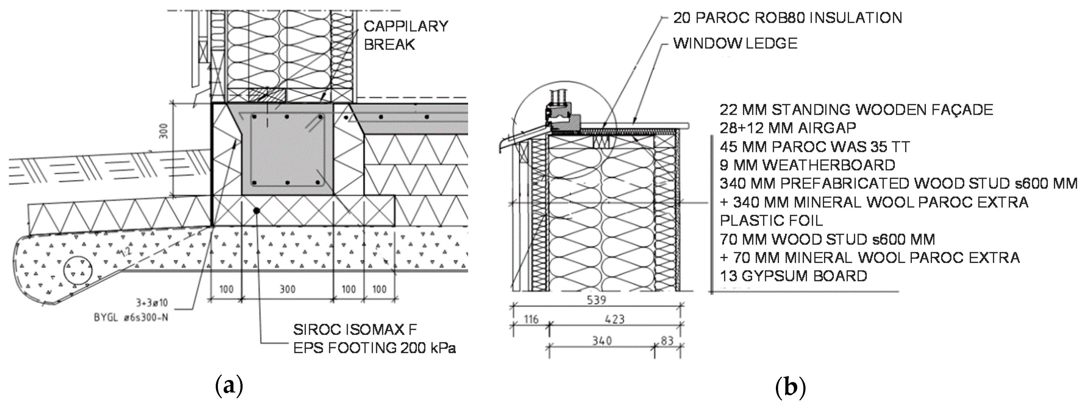
The slab on ground foundation has 300 mm of underlying expanded polystyrene (EPS), giving a U-value of 0.11 W/m
2K. The edge footing was designed with a prefabricated F-element in EPS (see
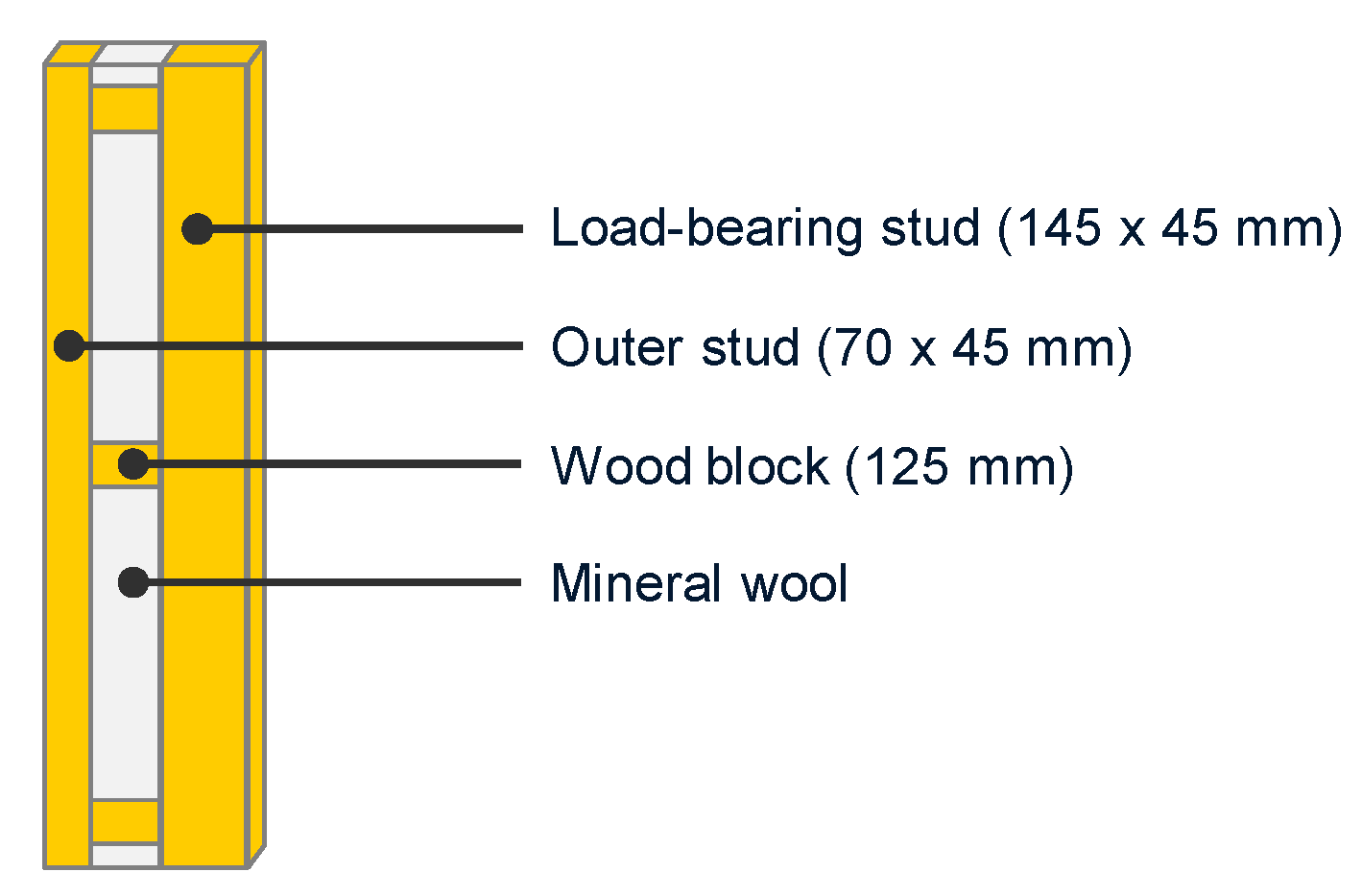
Figure 4). The external walls were constructed as prefabricated insulated wooden frameworks. In this project, a special stud was developed. It was constructed by assembling a 145 × 45 mm load-bearing wooden stud and a 70 × 45 mm outer wooden stud with 125-mm wood block distances, giving the assembled wall stud a width of 45 mm and a depth of 340 mm (see
Figure 6). This construction was chosen in order to minimize transmission heat transfer and keep the construction at a low weight.
The 340 mm × 45 mm wall stud was insulated with mineral wool. In addition, 45-mm insulation was added to the exterior side and 70 mm of insulated wooden framework was added to the interior side. This gives the construction a total insulation thickness of 455 mm and a thermal transmittance (U-value) of 0.09 W/m
2K. In order to minimize thermal bridges related to window-wall junctions, 20 mm of insulation was mounted prior to the window casings and window ledge (see
Figure 7). All insulation used for exterior walls was composed of rock wool. The roof construction was insulated with 500–600 mm of blowing wool (also rock wool) giving the construction a U-value of 0.07 W/m
2K. Windows and doors were mounted with a U-value of 0.90 W/m
2K and a solar energy transmittance of glass (g-value) of 0.50. The windows in the living rooms were given an external sun screen. The combination of window and external screen resulted in a g-value of 0.09. The external screen reduces the daylight transmission. Hence, the screen is primarily intended to be used on warm sunny days when the residents are not present.
The ventilation was designed with a mechanical balanced ventilation system with a heat recovery of 90%. The ventilation system has nominal ventilation, which gives the dwelling an air exchange rate of 0.5 air changes per hour (h−1). The ventilation system has the capacity to increase the air flow to 1.0 h−1, which may be done manually or programmed based on a chosen level of relative humidity or temperature.
A ground source heat pump was chosen to produce space heating and hot water. Heat for hot water is produced and supplied to a hot water storage tank. The SCOP of the heat pump used in the simulations was 3.0. The space heat is distributed via a floor heating system and supply air via heating coil in the ventilation unit.
During the summer, the boreholes are used as a natural heat sink. The working fluid for the heat pump is circulated in the boreholes cooling the working fluid, which then is used to supply cooling via a cooling coil in the ventilation system. A circulation pump is used, but no compressors are used for cooling.
Each building was designed with 40 PV panels measuring roughly 66 m2, giving each building an installed capacity of 10 kWp.
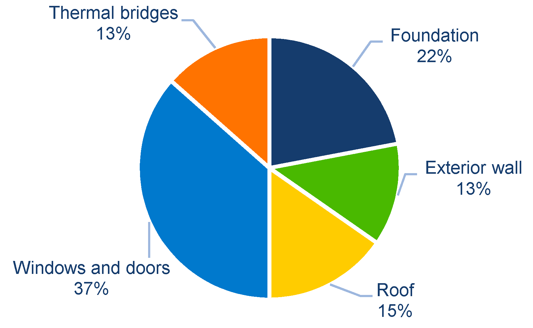
A summary of the technical description is given in
Table 3. The care for reducing thermal bridges resulted in low transmission heat losses via thermal bridges—13% based on the overall internal measurement (see
Figure 8).
4. Results
4.1. Results from Simulations
The simulations were based on the final design of the buildings and were presented previously [
36,
37]. The distribution of the energy use based on simulations is presented in
Table 4. The results from the simulations predicted an energy demand, excluding plug loads and lighting, of 29.8 kWh/m
2a. The PV panels were expected to generate almost 7900 kWh annually, which corresponds to 30.6 kWh/m
2a for the investigated building. It should be noted that the Net ZEB balance excludes energy use for plug loads and lighting (see
Table 1).
In the case study, the expected energy use for domestic hot water amounted to 6.7 kWh/m
2a, based on the normal energy demand for hot water use set to 20 kWh/m
2a and
SCOPDHW set to 3.0 (see
Table 3 and
Table 4). The hot water demand of 20 kWh/m
2a is not consistent with the Swedish regulations. This is due to the fact that that the design phase and simulations for the project were ongoing in the beginning of 2014, roughly two years before the regulations and values for normalisation were published.
It should be noted that electricity should be weighted with a factor of 2.5 according to the chosen Net ZEB definition, summarised in
Table 1. However, in this analysis no weighting factors are applied. The reason for this is twofold. Firstly, the building only demands and generates electricity; no other energy carriers are used. Secondly, the focus is to normalise and analyse energy performance. The authors believe that the results will be more transparent when showing the result without weighting factors.
4.2. Measured Results—Not Normalised
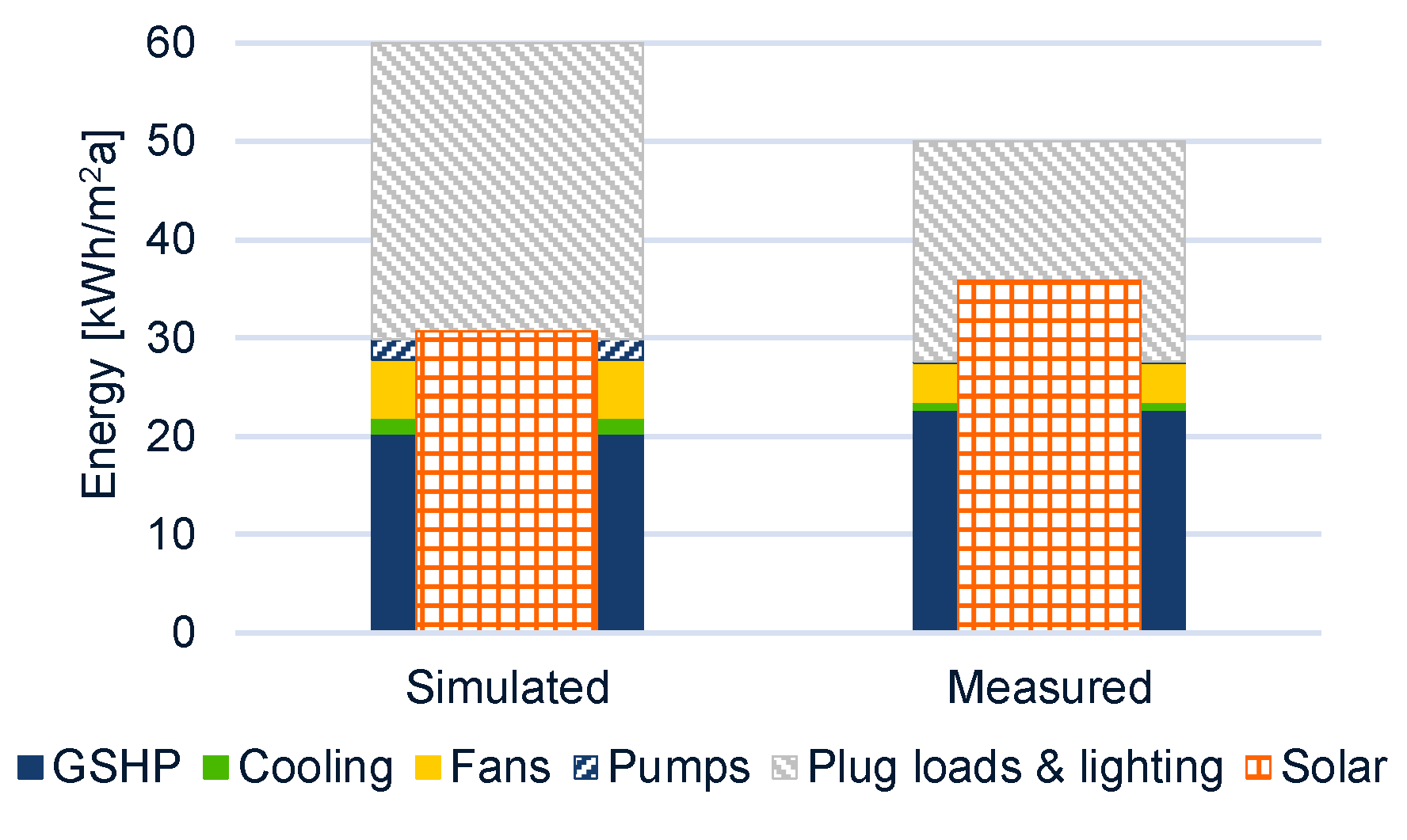
A comparison of simulated and measured results, not normalised, is presented in
Figure 9. The Net ZEB balance is reached and outperformed. The generated electricity from PV panels, normalised by the conditioned floor area, amounts to 35.7 kWh/m
2a, compared to a total energy demand of 27.6 kWh/m
2a (excluding plug loads and appliances). The measured energy use values for GSHP and generated energy from PV panels were both higher than predicted in the simulations. Energy use for fans, cooling, pumps, plug loads, and lighting were lower than predicted.
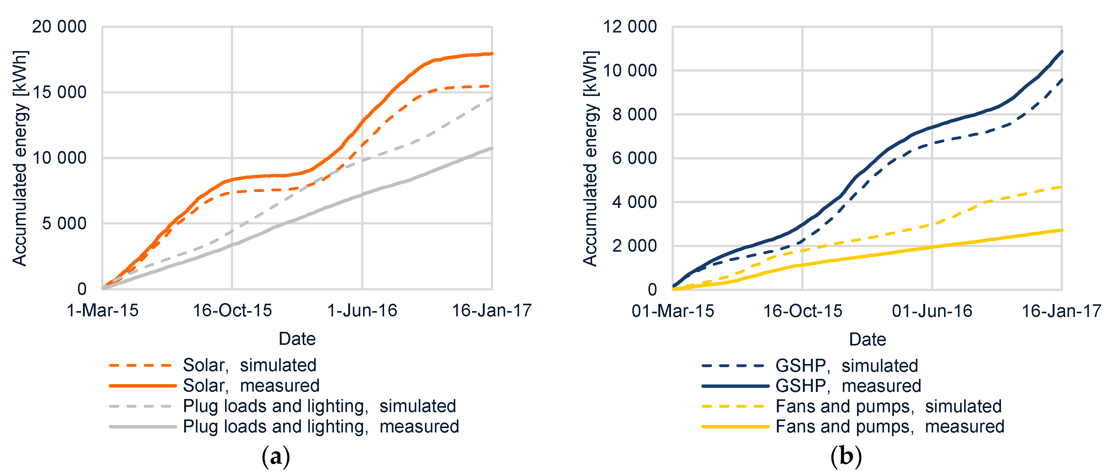
In
Figure 10, the accumulated energy demand and generation, both simulated and measured, are presented. The expected seasonal variation of generated energy from PV panels corresponds rather well with the results from the simulation. The clearest deviation of energy generated from PV panels is seen in autumn and winter, both for 2015 and 2016, where the generated energy outperforms the expectations from the simulation. Based on the year of 2016, the electricity values generated from the PV panels were 16.5% higher, as compared to those of the simulations.
The measured energy use due to plug loads and lighting is constantly lower than expected from the simulations. A slightly seasonal variation can be seen, but it is not as significant as assumed within the simulations. Based on the year 2016, the electricity use values for plug loads and lighting were 26.0% lower, as compared to the simulations.
With respect to the GSHP, the accumulated energy also follows a seasonal variation, which corresponds rather well with the results from the simulation. The clearest deviation is seen during summer, where the energy use is greater compared to the results from the simulation. Based on the year 2016, the electricity use for GSHP was 12.5% higher, as compared to the simulation.
Energy use for fans and pumps, including the pump that supplies free cooling during summer, is constantly lower as compared to results from the simulation. The expected increased energy use during summer due to increased ventilation and the use of free cooling is seen slightly during the first summer (2015), but not the second summer (2016). Based on the year 2016, the electricity use for fans, cooling, and pumps was 49.3% lower, as compared to the simulations.
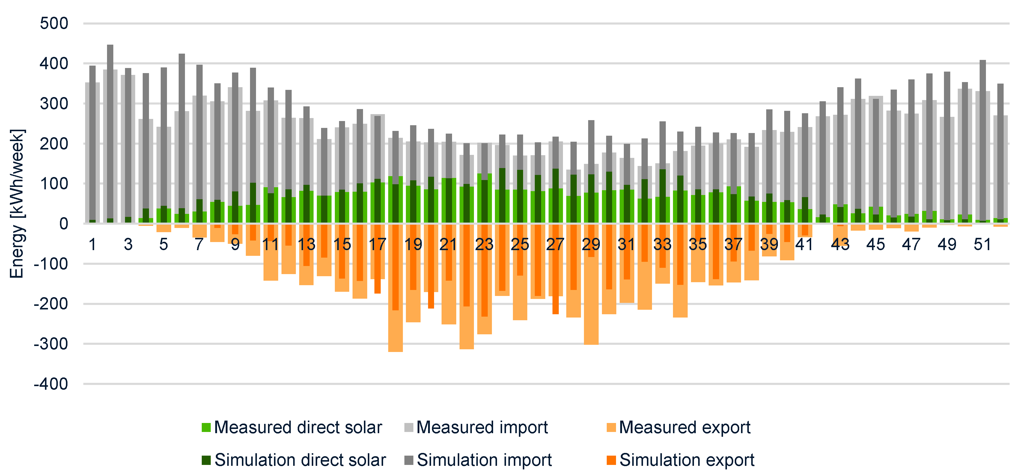
In
Figure 11, weekly results are shown regarding imported and exported energy, together with the direct use of solar energy. All values include energy use for plug loads and lighting. In the comparison, the slightly thicker and lighter bars represent measured data. The darker and narrower bars represent results from simulations. The time resolution is in hourly data, summarised for each week.
In general, the sums of direct solar energy use and imported energy were lower than predicted. However, the direct solar energy use values were usually below the values in the results from simulations. Over the year, the direct solar energy use was 12.0 kWh/m2a, as compared to the predicted 14.9 kWh/m2a. The measured values of import and export of energy were 38.1 kWh/m2a and 22.8 kWh/m2a, respectively, as compared to the values of 44.6 kWh/m2a and 15.7 kWh/m2a predicted using simulations. Thus, even though the energy demand was lower and the energy generation was higher, the direct use of solar energy was lower than predicted in the simulations.
4.3. Static Normalisation
To enable static normalisation, according to Boverket, values with respect to hot water use, indoor temperature (during heating season), plug loads, and lighting, as well as the energy index, were gathered.
Table 5 shows these results together with data to enable the normalisation of energy generation from PV panels. Monthly values are presented together with a summarised value for the whole year. Regarding indoor temperature, the value for 2016 is the average value, not a summarised value. Since the data are used for the normalisation of energy use for heating, data from May–August (in brackets), are not used.
The effect from the normalisation is presented in
Table 6. For each step, the total effect, including previous steps, are presented.
The first step, normalising energy use for domestic hot water, adjusts the measured result upwards. The measured result for domestic hot water shows an increase of 5.9%. However, the total increase in energy use for GSHP is less at 1.6%, since almost 70% of the energy use for the GSHP relates to space heating. The increase of the total energy demand is 1.3% after the first step. Since the normalisation is performed using absolute values, there is no difference between yearly or monthly normalisation.
The second step, normalisation due to deviating indoor temperature, results in the measured results being adjusted downwards due to higher indoor temperatures during the heating season as compared to the normal temperature. If adjustment for the total energy use for space heating is based on the average indoor temperature during the heating season, the measured energy use for space heating will be reduced by 5%. This is due to the fact that the average indoor temperature was 22 °C during the heating season. This results in a reduction of 3.6% for the GSHP. However, since the first step resulted in an increase of 1.6%, the result after the second step is a decrease of 2.0% for the GSHP.
If the normalisation is performed for each month separately, the decrease will only be 1.9%, resulting in a total decrease of 0.3% after the first two steps. The main reason for the differences in the normalisation is that the yearly normalisation is applied to all energy use for space heating (including the summer), whereas the monthly normalisation is only applied to energy use for space heating during the heating season.
The third step, normalisation due to deviating internal loads, is performed in absolute values (similar to the first step) and adjusts the measured results downwards since internal loads were lower when compared to normal use. The energy use values for plug loads and lighting were 7.7 kWh/m2a lower compared to normal use. Based on and of 70% and 3.0, respectively, measured results for space heating are reduced by 1.8 kWh/m2a, for both the monthly and yearly adjustment. The relative changes differ between yearly and monthly values due to different results from previous steps.
The fourth step, normalisation due to exterior climate, adjusts the measured results upwards due to lower energy index during measurements compared to the TMY. If the normalisation is based on the total energy index for 2016, it results in an increase of the energy use for space heating of 5.6%. Monthly normalisation results in an increase of the energy use for space heating of 5.9%. Since the GSHP also is used for domestic hot water, the adjustment is lower. Considering the first four steps, adjusting measured energy use for heating, yearly adjustment results in a reduction of measured energy use for GSHP by 6.5%, and the corresponding value for monthly adjustment is 4.6%.
In the fifth (and last) step, correction for energy generated from PV panels, there is an adjustment of measured energy downwards due to higher solar radiation during measurements compared to the TMY. The global radiation during 2016 was roughly 10% higher compared to a normal year. Hence, the measured generated energy from PV panels is reduced by roughly 9%. If normalisation is done separately for each month, the reduction is slightly lower.
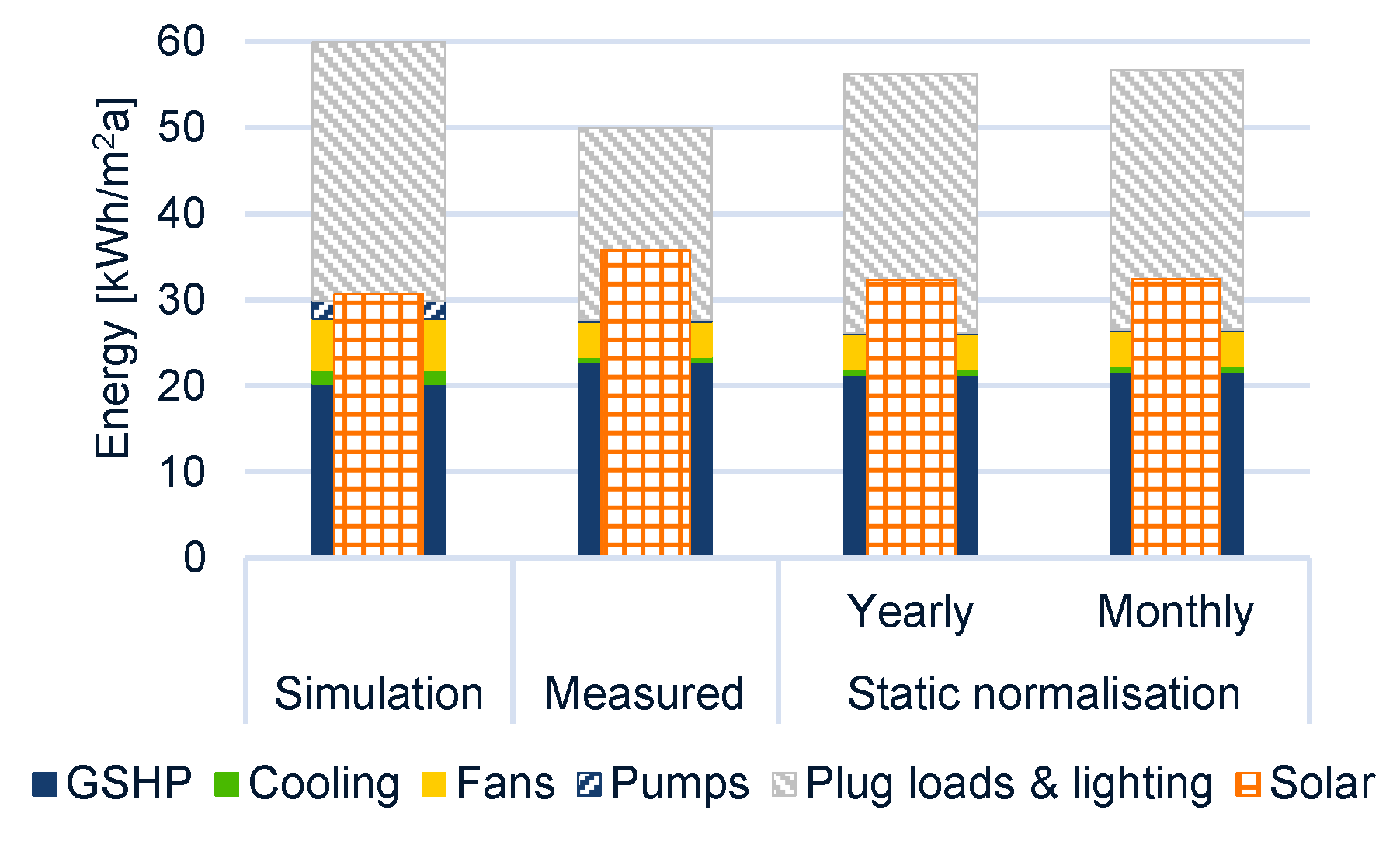
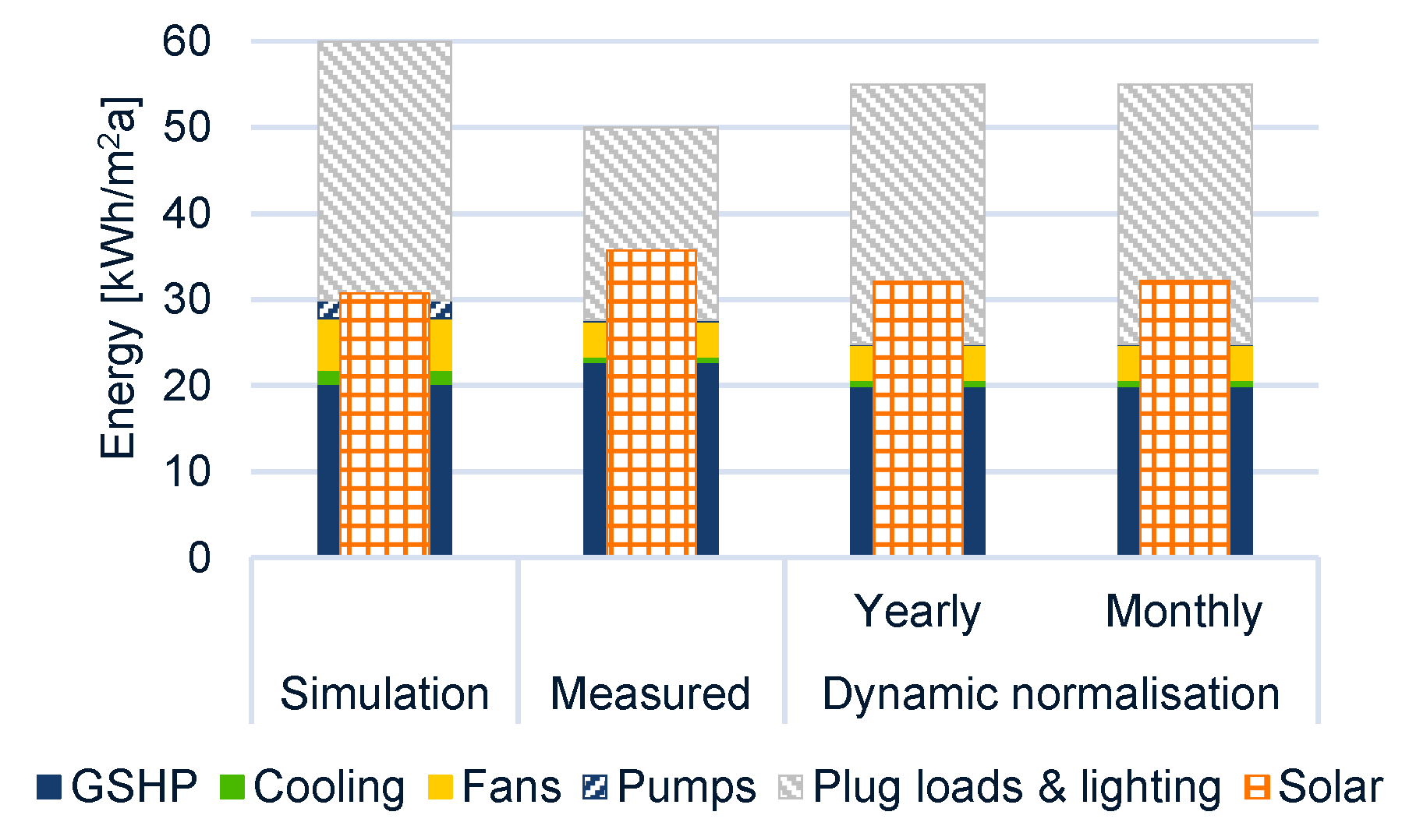
The results from the five steps are presented in
Figure 12. As can be seen, the difference between the final normalised results, comparing yearly and monthly normalisation, is low. Before normalisation, the measured energy use for GSHP was 12% higher as compared to the simulation. After normalisation, the corresponding values are 5.2% and 7.3% for yearly and monthly normalised values, respectively. The measured generated energy from PV panels was 16.5% higher compared to the simulation. After normalisation, the corresponding values are 5.5% and 5.8% for yearly and monthly normalised values, respectively. The largest relative deviation is with respect to energy use for cooling, fans, and pumps, which is not normalised.
4.4. Dynamic Normalisation
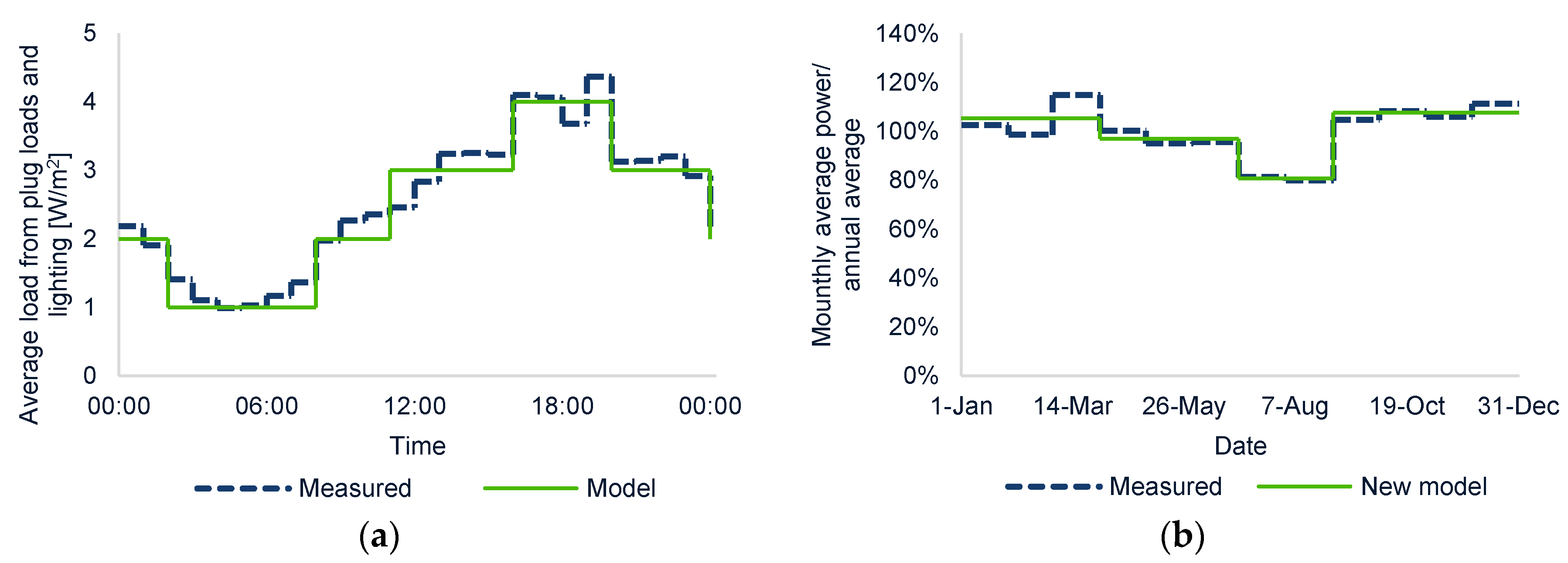
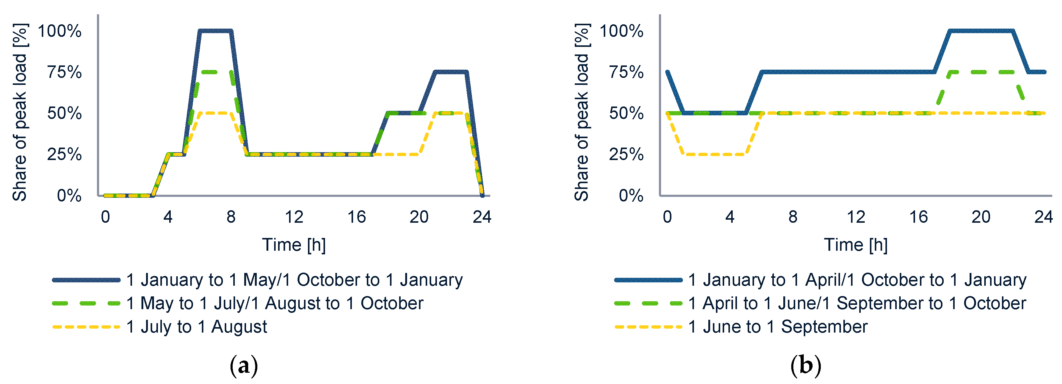
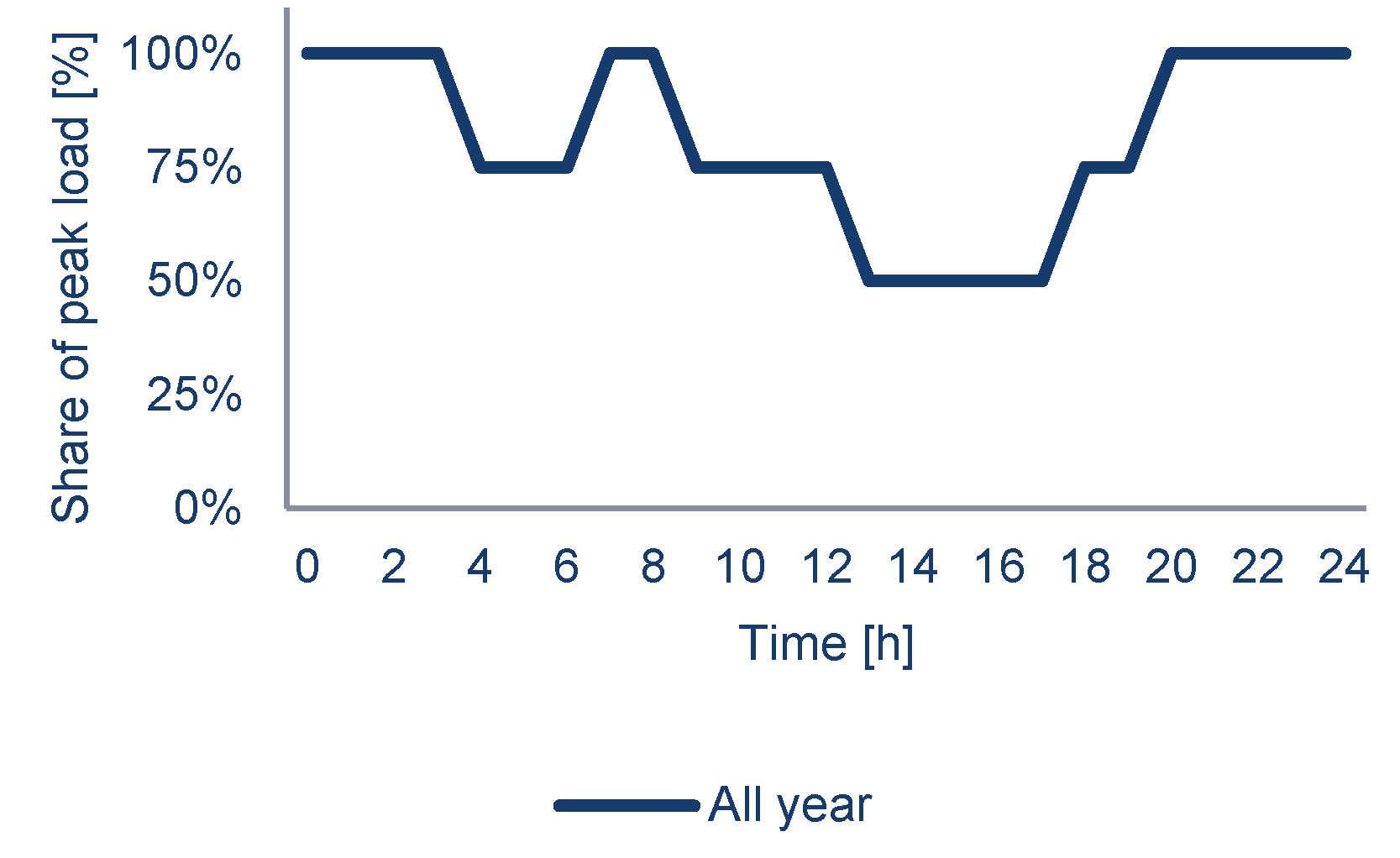
To enable dynamic normalisation, a new load profile for plug loads and lighting was needed. This profile was created based on the measured results. In
Figure 13, the daily and monthly variation is shown. The new load profile is a slightly simplified profile compared to the measurements. The new load profile results in the same annual energy demand as measured.
The dynamic normalisation, through repeated simulation, is carried out stepwise in the same steps as the static normalisation in the previous section. The results are presented in
Table 7.
The first step, normalisation of energy use for domestic hot water, gives the same result as that for static normalisation. The total energy use for GSHP is adjusted upwards by 1.6% and the total energy demand increases by 1.3% after the first step. There is no difference between yearly or monthly normalisation.
The adjustment for deviating indoor temperature (the second step) shows a rather high impact. When adjusting on a yearly basis, the reduction of the energy use for space heating is 16.0%. This reduces energy for GSHP by 11.4%, to a total reduction of 9.9% considering the first two steps. If adjustment is made on a monthly basis, the adjustment is slightly larger. The reduction for space heating is then 17.8%, resulting in a reduction of energy for GSHP of 12.6%, and thus a total reduction of 11.2% when considering the first two steps.
When applying the new load profile for plug loads and lighting in the third step, this results in a further reduction of the measured energy for space heating. The energy use for plug loads and lighting was reduced by 7.7 kWh/m
2a in the simulation, following the load profiles presented in
Figure 13 and
Figure 14. This resulted in an increased demand for space heating, disregarding the SCOP from the GSHP of 5.5 kWh/m
2a, which corresponds to an increase in space heating demand of 11.4% for a whole year. Applying the annual adjustment further reduces energy use for GSHP by 6.9%, leading to a total reduction of 16.1%. Monthly adjustment reduces the energy use for GSHP by 5.0%, leading to a total reduction of 15.6%.
The fourth step, normalisation due to exterior climate, adjusts the measured results for space heating upwards. The increase is higher if yearly adjustment is applied compared to monthly adjustment. The total adjustment of GSHP, considering all four steps and comparing yearly and monthly adjustment, is almost the same, with a reduction of roughly 12%.
The fifth (and last) step, when the energy generation from PV panels is adjusted, results in a reduction of measured generation of roughly 10%.
The results from the five steps are presented in
Figure 14. As can be seen, there is almost no difference between the final normalised results, comparing yearly and monthly normalisation. Before normalisation, the measured energy use for GSHP was 12.5% higher as compared to the simulation. After normalisation, the corresponding values are −1.1% and −1.3% for yearly and monthly normalisation, respectively. The measured generated energy from PV panels was 16.5% higher compared to the simulation. After normalisation, the corresponding values are 4.6% and 4.8% for yearly and monthly normalisation, respectively. In the same way as for the static normalisation, energy use for cooling, fans, and pumps has not been normalised.
5. Discussion
Within this study, the quantity and/or presence of residents was not documented. This causes some uncertainty in the results, as the effect from predicted versus actual heat gains from occupancy are not included in the normalisation. Furthermore, since the equipment for measurements was calibrated and installed by sub-contractors, the authors did not control the calibration. However, the tests of the normalisation methods bring up interesting aspects for discussion.
Regarding the normalisation of energy use for hot water, this adjustment had the lowest effect as compared to the other adjustments. There are no differences in the results when comparing the static and dynamic normalisation. This is due to the fact that that the simulation software considers the domestic hot water demand and the assumed SCOP for the heating production for hot water to calculate energy use for domestic hot water production. As such, the effect of the hot water storage tank was not included in the simulation. Furthermore, the production of heat for hot water was not measured (only the quantity of hot water use was measured). Therefore, it was not possible to evaluate and analyse the SCOP for hot water production. Hence, the energy use for hot water was based on quantities of hot water use and not measured energy use. This is a weakness which gives the results from the study some uncertainty. Upcoming studies of similar projects should widen their measurements in order to give more certainty to their results.
Normalisation due to indoor temperature showed the largest difference when comparing static and dynamic normalisation. The dynamic normalisation resulted in a reduction of 16.0% and 17.8% for the space heating demand, where the lower value was based on yearly adjustment. These results correspond rather well to previous studies [
10,
16,
18], which showed increased energy use for heating of around 12.2% to 20.0% when indoor temperatures were increased by 1 °C within the indoor temperature interval of 20–25 °C. Other studies showed a lower impact, from 8.0% to 10.0% per °C [
7,
38]. Regardless, no study showed an impact of 5% per °C, which indicates that the recommended adjustment of 5% per °C given in the Swedish regulations is low. It should be noted that the studies included above are passive-/low-energy houses. This means that the absolute deviation may be considered to be low, between 1.5 and 3.0 kWh/m
2a.
The effect of deviating the use of plug loads and lighting showed a rather high impact, both for static and dynamic normalisation. The dynamic normalisation showed that a reduction of heat gains from plug loads and lighting by 7.7 kWh/m
2a resulted in an increased heating demand of 5.5 kWh/m
2a. This corresponds well to the share of internal loads assumed to affect heating or cooling, given by Boverket, of 70% [
22]. In this case, the static normalisation resulted in an adjustment of energy demand by 5.4 kWh/m
2a (70% of 7.7 kWh/m
2a). Based on a SCOP of 3, the adjustment for energy use for GSHP was 1.8 kWh/m
2a. The result did not differ between yearly or monthly adjustments since the adjustment was in absolute values. The dynamic normalisation, which used the ratio between simulations for step 2 and step 3 as an adjustment factor, resulted in a lower adjustment compared to the static normalisation. The adjustment of energy use for GSHP was 1.4 kWh/m
2a and 1.0 kWh/m
2a, for yearly and monthly normalisation, respectively. This indicates that an adjustment of energy use due to deviating internal loads may give a more accurate result conducted in absolute values.
Regarding normalisation due to deviating exterior climate, these adjustments were the second-lowest of the adjustments. The adjustments were also relatively equal, regardless if they were normalised by the static or dynamic method, with yearly or monthly adjustment. Except for the normalisation of hot water, normalisation due to deviating exterior climate showed the smallest difference between static and dynamic normalisation. This indicates that normalisation by energy index is a static normalisation which gives realistic results.
Differences regarding the two methods for normalisation of energy generation from PV panels were low. This is most likely due to the fact that both methods were based on monthly deviations based on data from SMHI. Upcoming studies of similar projects should widen their measurements in order to provide greater certainty of their results.
Comparing the static and dynamic normalisation, dynamic normalisation resulted in a normalised value for GSHP closer to the predicted energy demand than did static normalisation. The measured and dynamically normalised energy demand values for GSHP were roughly 1% lower than those found in the results of the simulation, as compared to static normalisation where the measured and normalised energy demand was approximately 5–7% higher. The measured and dynamically normalised energy generation values from PV panels were roughly 4% higher than those found in results from simulations, as compared to static normalisation where the measured and normalised energy generation was roughly 5% higher.
The deviation of energy use for fans and pumps was rather high, almost 50% lower compared to the results from the simulation in the design phase. The deviation was mainly due to the better performance of fans and pumps, not deviating boundary conditions such as a greater use of increased/forced ventilation, etc.
6. Conclusions
Monitoring energy use is important to ensure that predicted energy use is achieved in the actual use of buildings. This study shows that it is important to normalise the measured energy use in order to determine an accurate energy performance. The normalisation of measured energy use may, to a large extent, close performance gaps and explain deviations between simulations and measurements, and thus between predictions and reality.
It is important that the normalisation not only considers deviation in exterior climate. Therefore, the monitoring of energy use should always be done in a way that enables normalisation for important parameters. Such parameters, highlighted in this study, are the use of domestic hot water, indoor temperature, internal loads, and outdoor climate. Measurements of outdoor climate should include at least outdoor air temperature, relative humidity, wind speed, and solar radiation.
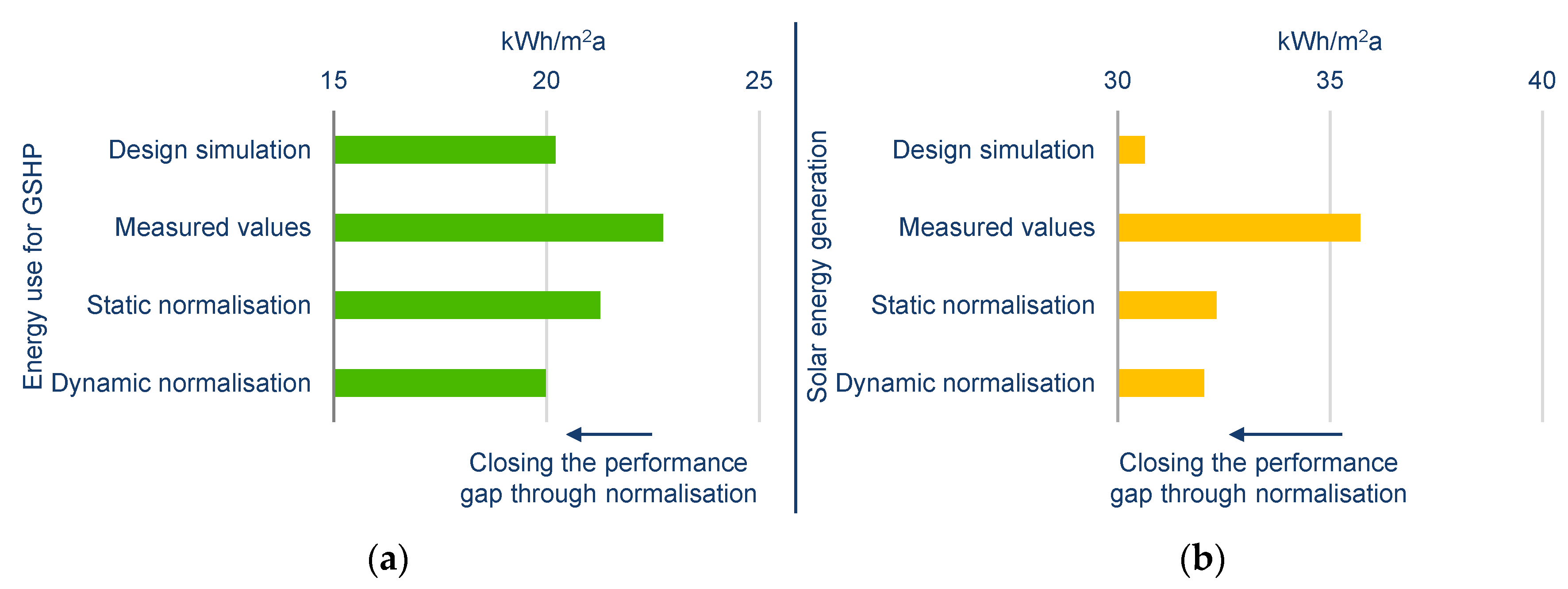
This study normalises the energy use for heating, hot water, and solar energy generation. This includes the energy use for the GSHP (used for both heating and hot water) and the generated energy from the PV panels. Before normalisation, the performance gap between the design simulation and measured energy use for the GSHP was 2.5 kWh/m
2a, which corresponds to 12%. The static and dynamic normalisation reduced the performance gap (based on yearly adjustment) to 1.5 kWh/m
2a and −0.2 kWh/m
2a, respectively, which corresponds to 5% and −1%. The normalisation of energy generation from PV panels reduced the performance gap from 5.1 kWh/m
2a to 1.7 kWh/m
2a and 1.4 kWh/m
2a, for static and dynamic normalisation, respectively (based on yearly adjustments), which corresponds to a reduction of the performance gap from 17% to 5%, for both static and dynamic normalisation (see
Figure 15).
This study shows that the dynamic normalisation of heating gives normalised values closer to those predicted in the simulation, as compared to static normalisation. However, this study is only indicative since it is based on a single case. More studies are needed to investigate which normalisation method will give more accurate results.
The static method for normalisation is simple and straightforward. Hence, it is also feasible for use in other countries with similar boundary conditions. The static method should be easier to use compared to more complex methods such as dynamic normalisation and calibration of energy models. However, more research should be done to verify and improve the method. Normalisation due to indoor temperature showed the largest difference, comparing static and dynamic normalisation. Further verifications and improvements could start there. Further research and development should also investigate how to include the normalisation of more parameters. Examples include heat gains from occupants and cooling energy use due to internal heat gains and solar radiation.
Finally, this study shows that it is possible to build a Net ZEB in a Swedish climate with technologies existing on the market today. However, the import-export electricity balance is hard to predict, even if dynamic simulations are conducted with detailed load profiles.


