1. Introduction
In the European Union, the energy consumption of buildings accounts for around 40% of the final energy consumption, and about 75% of existing buildings are considered to be energy inefficient.
The energy performance of buildings in the European Union is regulated by Directive 2010/31 [
1]. Both new buildings and rehabilitated buildings must meet the minimum energy performance requirements, which are set according to climatic and local conditions. There are also recommendations for the reduction of carbon dioxide emissions and for increasing the share of the energy provided by renewable energy sources [
2,
3]. In line with the requirements for new buildings, support policies are recommended to shift the refurbishment of existing buildings towards nearly zero-energy buildings (nZEBs) [
4]. The nearly zero—or very low amount of—energy that is required should be covered to a significant extent by renewable energy sources that are produced on-site or nearby. Authors in [
5] analyse the construction features of a set of nZEBs that were collected from 17 European countries. An increasing amount of papers that have been published in recent years consider the nZEB concept [
6,
7,
8].
Reducing the energy consumption—and hence the carbon dioxide emissions—of buildings is an important way to minimize the environmental impact. Thus, the need to refurbish existing buildings provides an opportunity to improve the energy performance of buildings.
An energy audit—with the aim of identifying optimal solutions in order to increase the energy performance—is required for the refurbishment of a building. The audit is necessary in order to identify optimal energy efficiency solutions. The refurbishment project must take into account both the envelope and the building’s services [
9,
10,
11]. The cost–benefit analysis is generally used for the evaluation of the rehabilitation measures [
12,
13]. However, it is also recommended to consider the carbon dioxide emissions [
14].
In most cases, a building’s energy sources are considered and analysed individually. A joint examination (as opposed to an individual examination) can lead to numerous benefits, such as continuity in energy supply, supply flexibility, and optimization potential.
Given that several sources of energy can be used to meet the energy demand of the building’s utilities, the availability of energy for the required loads (electricity, heat, and cooling) is no longer dependent on a single infrastructure. The increased flexibility in energy supply is because of the redundant ways of covering the load curve, in which some degree of freedom is provided.
The optimization potential stems from the fact that several sources of energy, and various combinations thereof, can be used to meet the requirements of consumers at a lower cost.
Typically, the optimization methods are used on systems with a single form of energy, such as electricity, natural gas, or district heating. The energy hub concept allows for the determination of an optimal interface between certain energy infrastructures and loads. An integrated system of the energy sources can make use of multiple paths to deliver different forms of energy. Recently, there has been an increased interest in concerns surrounding the modelling and combined analysis of multi-carrier energy systems [
15,
16,
17,
18]. The energy sources that are used can be characterized by the different costs, related emissions, availability, and other criteria [
19,
20,
21,
22]. Nižetić et al. [
23] present different hybrid energy scenarios for application in small or medium-sized residential building facilities in typical Mediterranean climate conditions. The concept of levelized cost of electricity (LCOE) is used to compare the cost of energy that is provided by different sources.
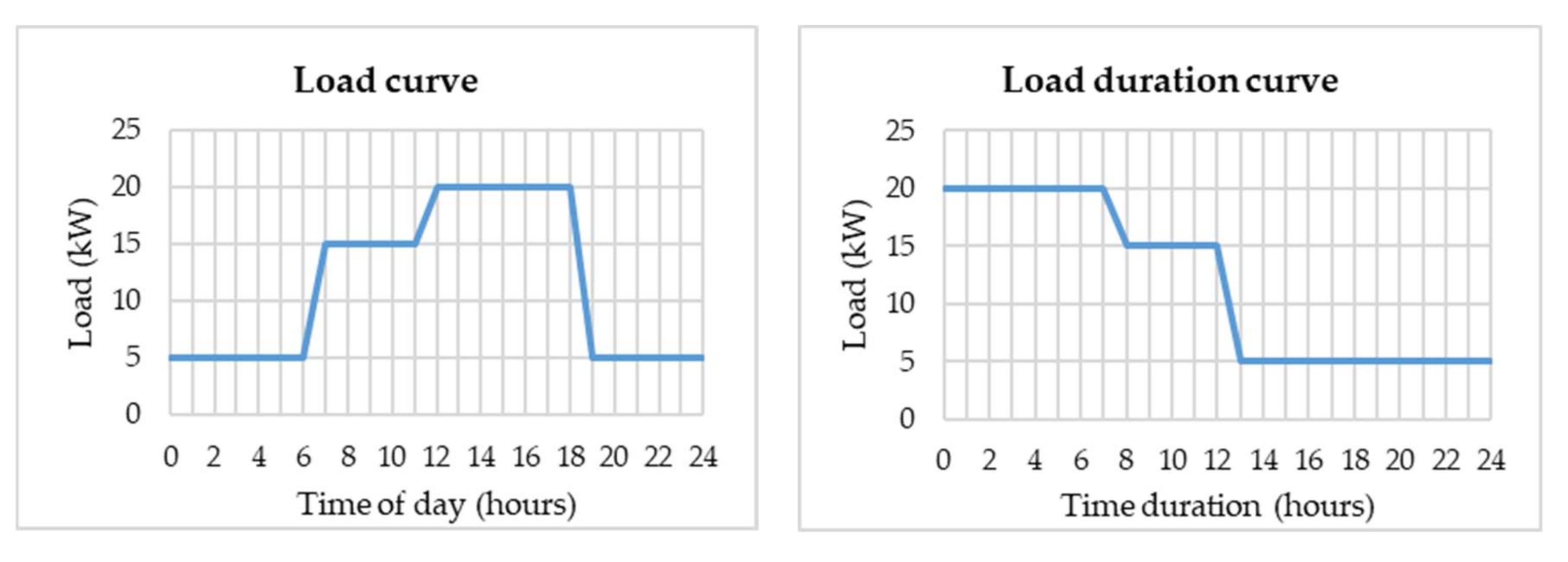
The correct determination of the consumption curves of the building is of great importance for the choice of energy sources [
24,
25,
26]. The consumption curve, or load profile, is a chart that illustrates the variation in the demand for energy over a specific period of time. The load duration curve is derived from the chronological load curve. An example of deriving the load duration curve for one day is presented in
Figure 1. The analysis period may be extended to either one week, one month, or one year. The information is the same in each case, but it is presented in different forms. These curves are useful in the selection of generation technologies, in order to plan how much power they will need to generate at any given time.
In this paper, a method of choosing the energy sources that are required for the building’s utilities (electricity, heat, and cooling) is developed. In
Section 2, the mathematical model that was used—based on the concept of the energy hub—is presented. The details of the proposed optimization framework are described in
Section 3. The case study is then introduced and described, along with the assumptions and input data for a non-residential building (office building). The evaluation of energy use and the economic analysis for each of the scenarios for the target building are then carried out. Finally, in
Section 4, the conclusions are presented.
The main objective of this paper is to select the energy sources (electricity, heat, and cooling) that are required for the following building utilities: lighting, appliances, domestic hot water, heating, ventilation, and air conditioning.
2. The Mathematical Model that Was Used
The energy that is required for a building's utilities (lighting, domestic hot water, heating, ventilation, and air conditioning) is provided by energy carriers from various sources—either directly or through conversion systems that convert energy from one form into another. An energy carrier is an energy form that can be converted to other forms at a later stage, such as mechanical work, electricity, heat, or cold. An energy carrier corresponds only to an energy form (and not to an energy system) of energy input that is required by the building’s utilities. The economic analysis of the application of the various power supply solutions of a building involves the determination of the net present value of the overall costs that are involved in making investments and operating the building’s services over the life of the investment, as well as the quantification of the carbon dioxide emissions.
The objective function is described as the overall cost of all of the forms of energy that are consumed in the building at the net present value as follows:
where:
C0 represents the initial investment costs (EUR);
CE is the annual cost of energy that is consumed at the reference year level (EUR/year);
CM is the annual operating and maintenance (O&M) cost (EUR/year);
CCO2 is the annual cost of carbon dioxide emissions (EUR/year);
f is the annual rate of increase in the cost of energy;
i is the discount rate;
k is index corresponding to the energy source that is used;
N is the calculation period.
To estimate the overall costs, it is necessary to know the power that is installed and provided by the energy production technologies that are inside the building, as well as the required capacity from outside energy sources. The interactions between these energy systems were considered based on the concept of the energy hub [
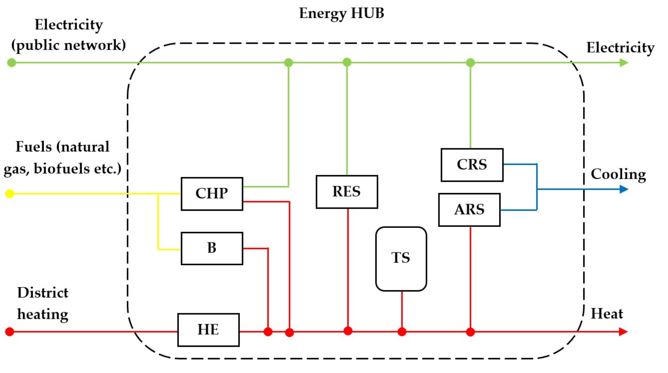
27]. Mathematically, this is a mixed-integer linear problem (MILP), which can be easily solved using classic mathematical techniques. An energy hub is the interface between the transport infrastructure (networks), local sources, and energy consumption (loads) in the building.
For example, the electricity that is required by consumers in the building can either be provided by the public electricity grid, produced locally in a cogeneration plant, or produced using renewable energy sources (solar, wind). Similarly, different feed solutions can be considered for the other utilities that are used in the building (heating, cooling) (
Figure 2). Thus, the energy requirement in the building can either be secured directly from the appropriate entrance or may be generated partially or totally within the energy hub. By using such an approach, an unattractive energy carrier (for example, one with a high cost or high carbon dioxide emissions) can be substituted or even eliminated.
The multi-carrier energy system can be described by the following matrix equation [
27,
28]:
where:
α, β, …, ω are the different energy carriers;
L is the load matrix (the energy consumption of the building);
P is the power matrix of the energy carriers that enter the hub;
C is the converter coupling matrix.
Thus, after applying Equation (2), the power balance equation can be reformulated as follows:
The coupling coefficients characterize the energy efficiency of conversion as follows:
where
is the dispatch factor that represents the percentage of input power
Pi and
is the conversion efficiency of energy carrier
i.
The constraints for the dispatch factors are as follows:
The coupling matrix between the energy carriers reflects the degrees of freedom that can be used to optimize the energy requirement in the building.
The input power of the converter is given as follows:
The energy storage can be modeled similarly to that of a converter device. The energy that is stored after a certain operating period
T equals the initial storage content plus the time integral of the power:
The factor
is considered to be the charge/discharge efficiency and depends on the direction of the power flow:
Different mathematical constraints can be identified in the proposed model: the conversion capacity; the storage capacity; the minimum production from renewable energy sources; and the energy content at the initial time period (
t = 0) must be equal to the energy content at the last time period (
T):
Therefore, the objective function (1) is associated with two types of constraints, namely, equality constraints corresponding to energy balance equations and inequality constraints corresponding to the limits of the conversion systems and the energy carriers that are entering the hub.
3. Example Application
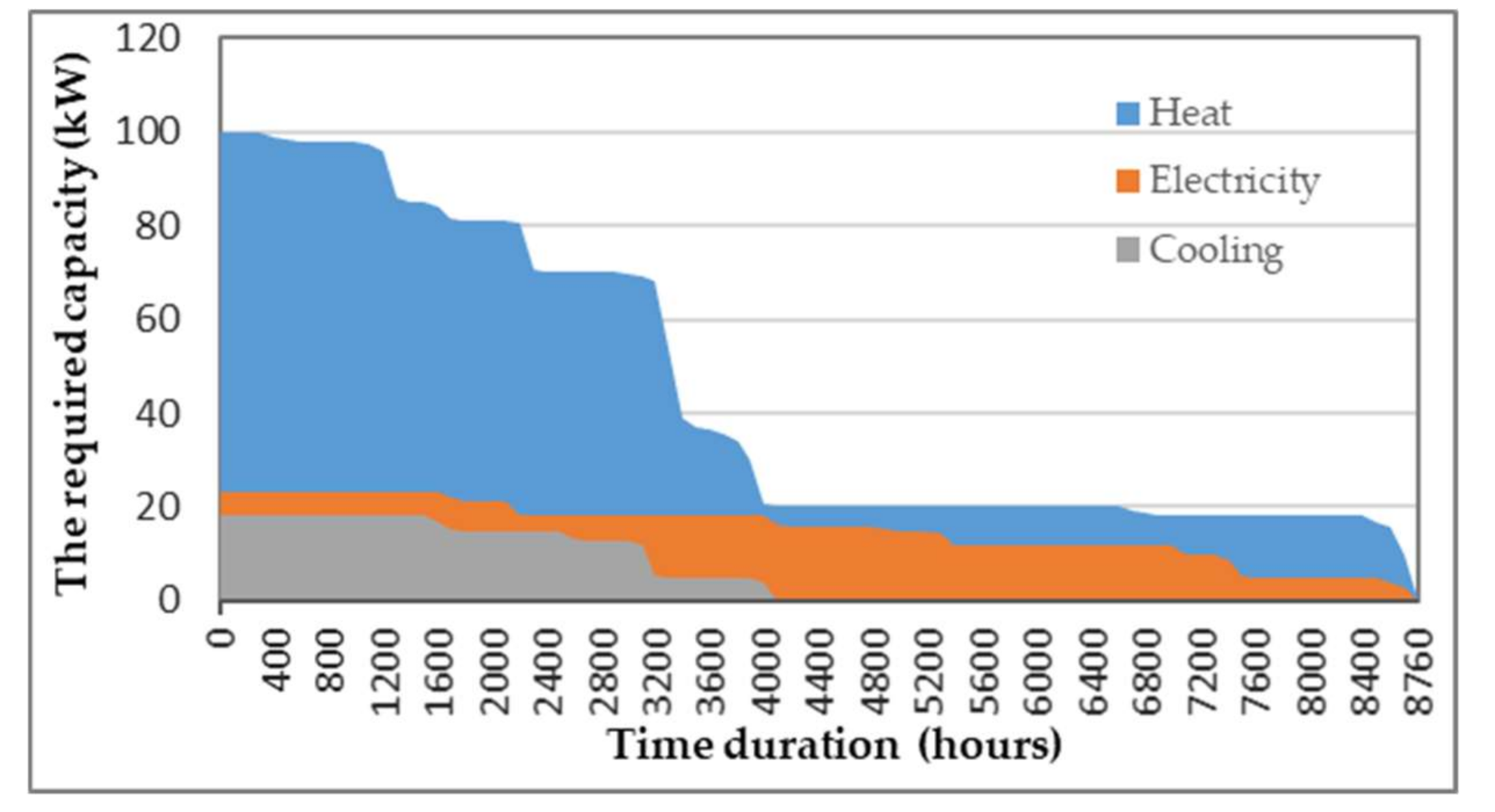
A non-residential building (office building) that was proposed for refurbishment—with four floors (each 3 m in height) with an S/V ratio of 0.31 and a total useful floor area of 4680 m
2—was investigated. The building is located in the northeastern part of Romania. The annual energy demands (heat, electricity, and cooling) resulting from interventions to the building envelope (external wall thermal insulation, thermal insulation of the upper and lower floors, and the replacement of existing windows and doors) is shown in
Figure 3. The mean U value of the envelope is 0.39 W/m
2K (the U-value of the wall is 0.41 W/m
2K; the U-value of the roof is 0.20 W/m
2K; the U-value of the basement is 0.24 W/m
2K; and the U-value of the glass is 1.30 W/m
2K).
The energy loads that are presented in
Figure 3 (electricity, heat, and cooling) include all of the energy requirements of the building, namely lighting, domestic hot water, heating, ventilation, and air conditioning.
The following scenarios were considered in order to ensure that the energy demands (heat, electricity, and cooling) are met in the case of the analysed building:
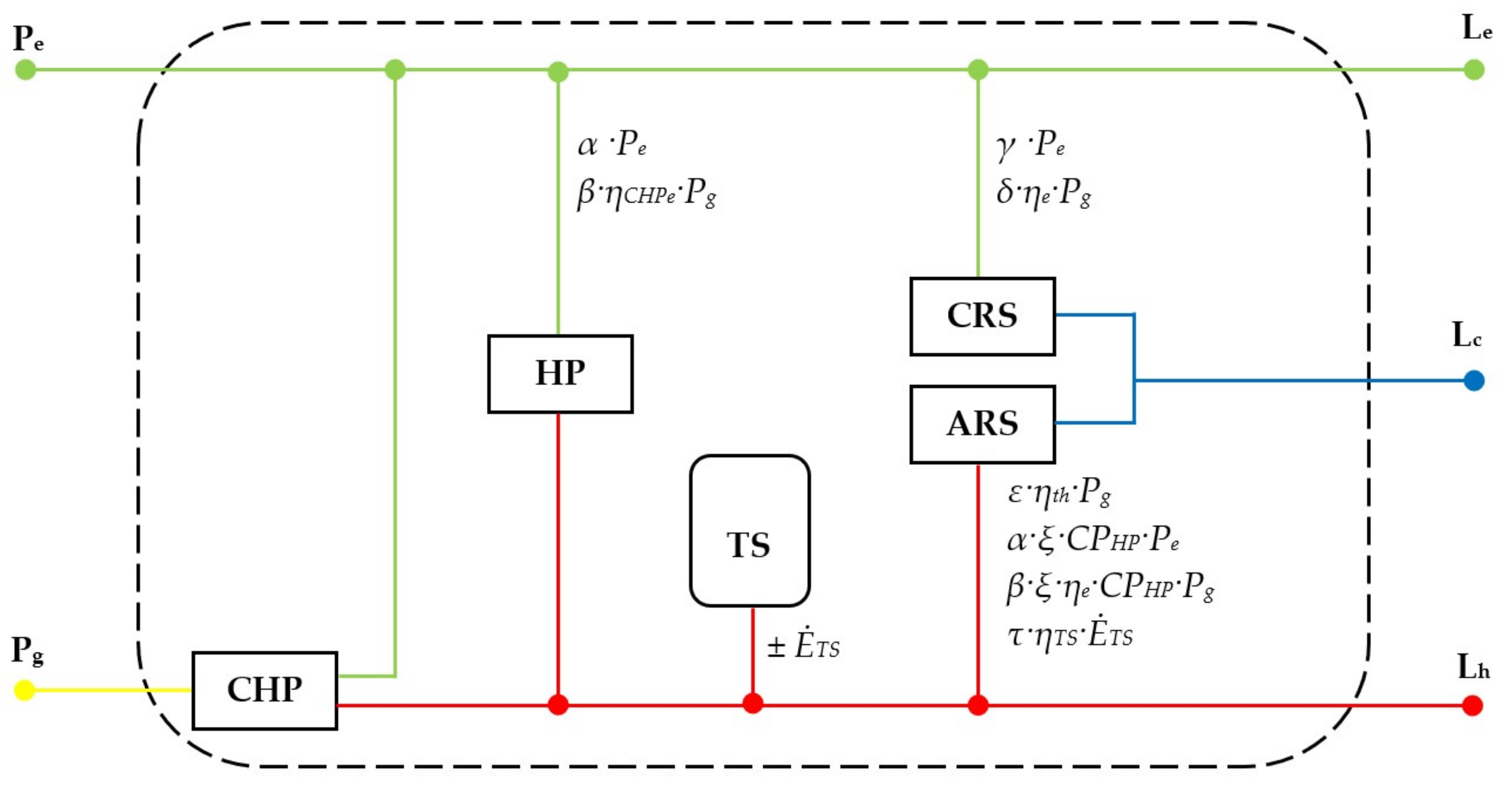
Scenario 1 (
Figure 4) includes the following energy sources: the electricity supply from the public network; two combined heat and power plants (CHPs) on natural gas fuel; a heat pump; a heat storage system; a compression refrigeration system; and an absorption refrigeration system.
Scenario 2 (
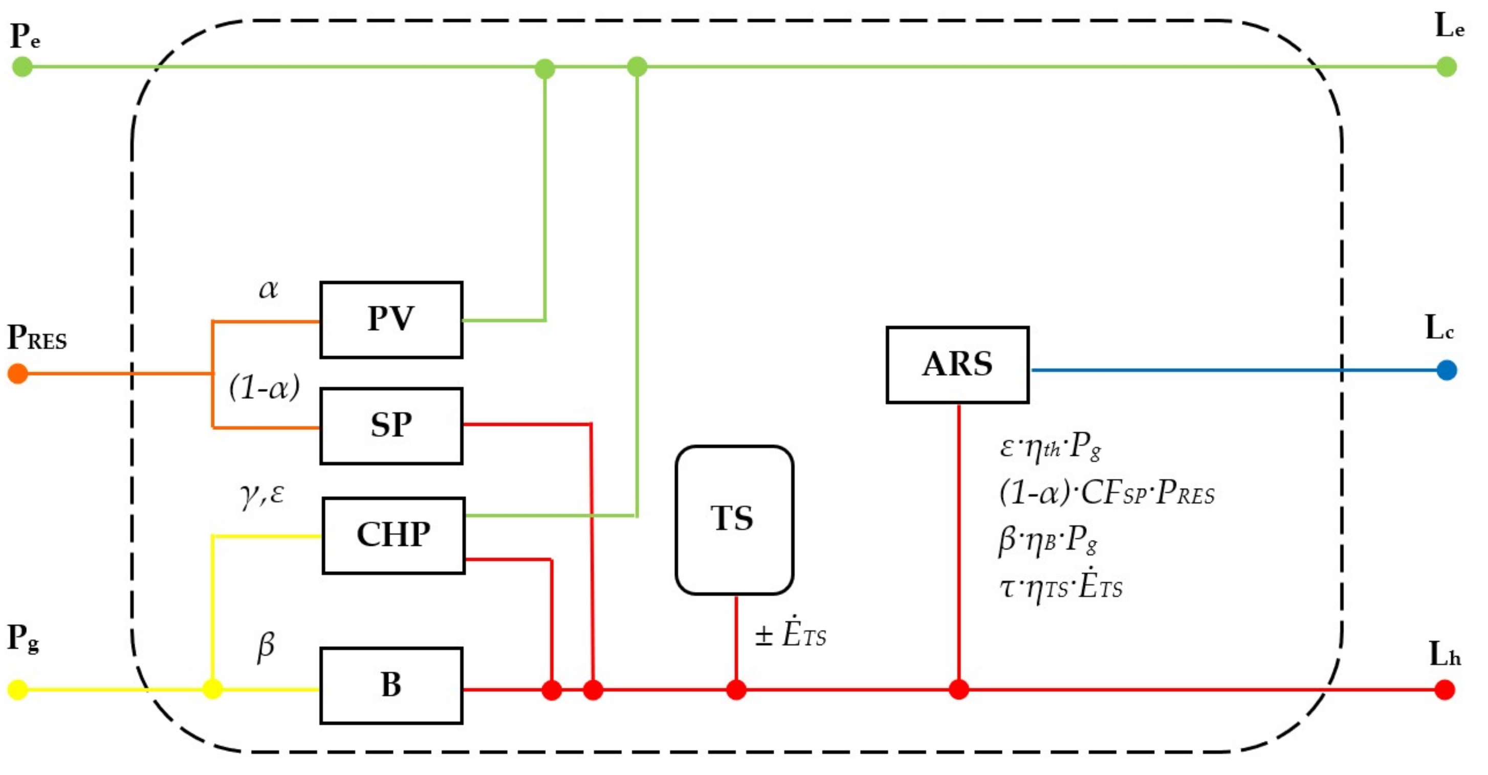
Figure 5) includes the following energy sources: the electricity supply from the public network; a combined heat and power plant (CHP) on natural gas fuel; a natural gas boiler (as a peak source); a system of photovoltaic panels; a system of solar thermal panels; a heat storage system; and an absorption refrigeration system.
Scenario 3 (
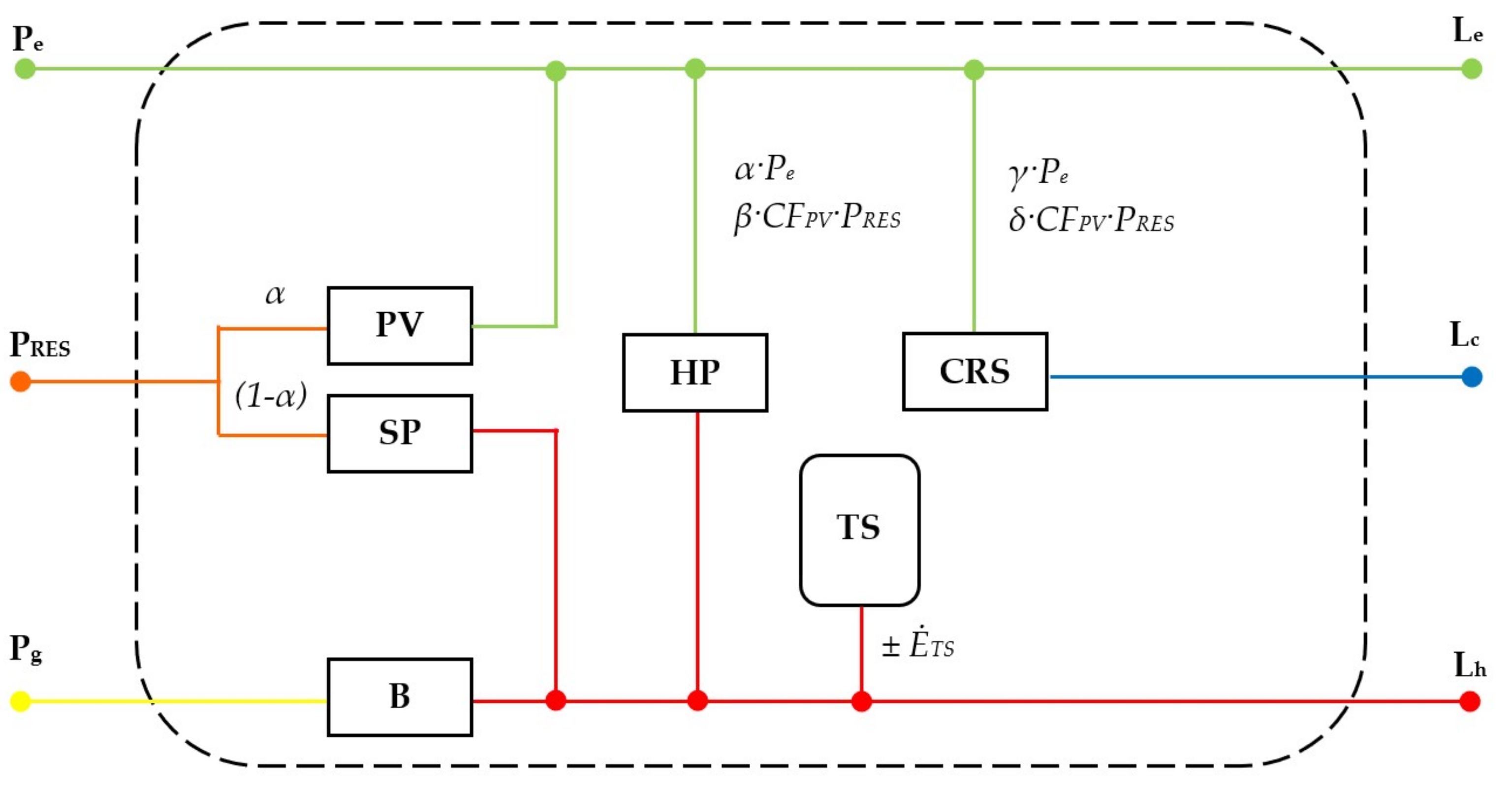
Figure 6) includes the following energy sources: the electricity supply from the public network; a heat pump; a natural gas boiler (as a peak source); a system of photovoltaic panels; a system of solar thermal panels; a heat storage system; and a compression refrigeration system.
Scenario 4 (
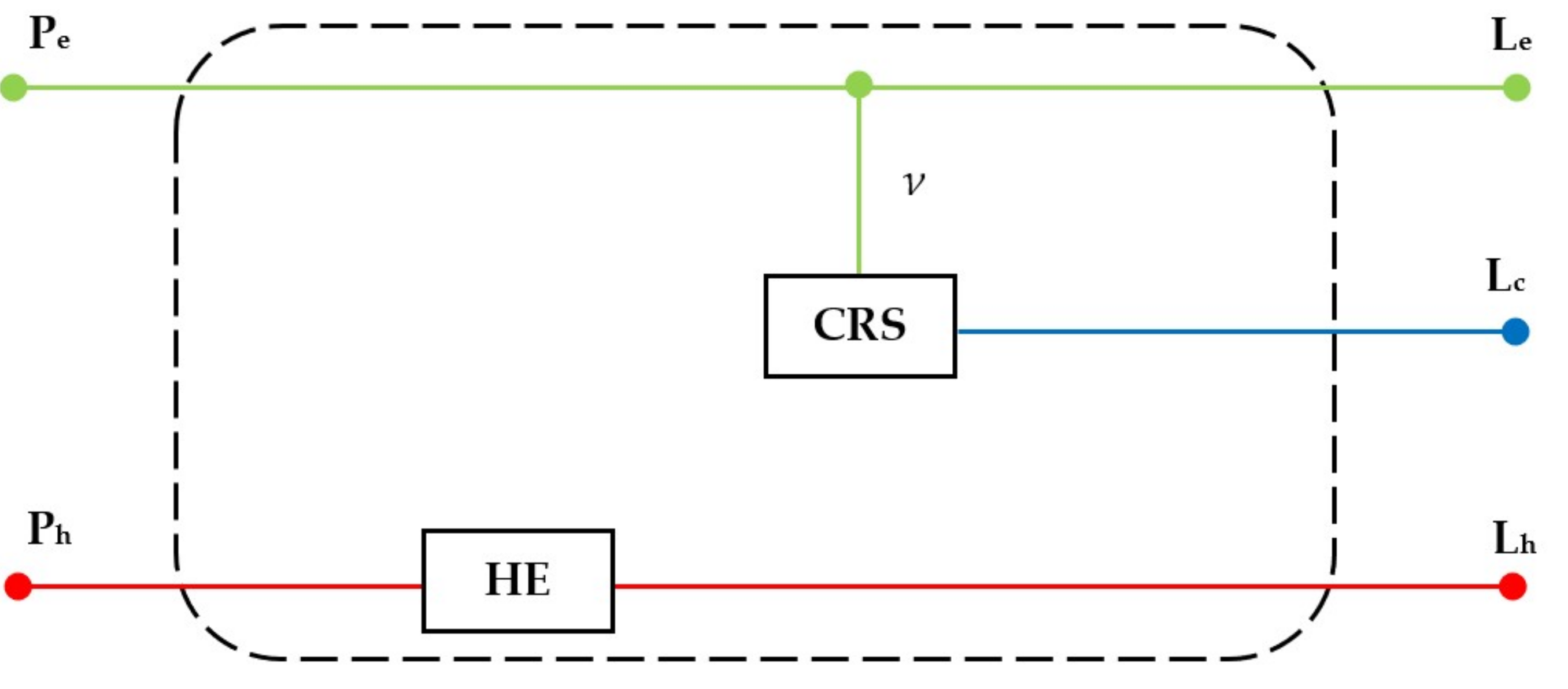
Figure 7) includes the following energy sources: the electricity supply from the public network; the heat supply from the district heating system and a compression refrigeration system.
In Scenario 1 (
Figure 4), the demand for electricity will be fulfilled by the cogeneration plants and the public electricity network. The cold demand will be fulfilled by the absorption refrigeration system or the compression refrigeration system (depending on the heat that is available from the cogeneration plants). The demand for heat in the building is fulfilled by the heat pump and the cogeneration plants. The type and size of the cogeneration plants is chosen according to the level of heat consumption. The electricity differences between local consumption and production are compensated for—without technical difficulty—by the public electricity network. The absorption refrigeration system can consume the available heat that is produced in the cogeneration plants, and consequently increases the efficiency of the cogeneration solution. The heat storage system will be used to compensate for the load variations and to increase the flexibility of the cogeneration plants.
Equation (2) customized for Scenario 1:
where
α, β, γ, δ, ε, ξ, and
τ are the dispatch factors:
α is the share of electricity to supply the heat pump;
β is the share of natural gas that is converted into electricity to supply the heat pump;
γ is the share of electricity to supply the compression refrigeration system;
δ is the share of natural gas that is converted into electricity for the compression refrigeration system;
system;
ε is the share of natural gas that is converted into heat for the absorption refrigeration system;
ξ is the share of heat from the heat pump for the absorption refrigeration system;
τ is the share of heat that is stored to supply the absorption refrigeration system.
and the efficiencies of the converters are as follows:
ηe is the efficiency of electricity generation in cogeneration;
ηthis the efficiency of heat generation in cogeneration;
CPHP is the coefficient of the performance of the heat pump;
CPCR is the coefficient of the performance of the compression refrigeration system;
CPAR is the coefficient of the performance of the absorption refrigeration system;
eTS is the storage efficiency of thermal energy—Equation (8).
The performances of the different energy sources that were considered in Scenario 1 are presented in
Table 1 [
29,
30,
31].
In Scenario 2 (
Figure 5), the demand for electricity will be fulfilled by the system of photovoltaic panels, the cogeneration plant, and the public electricity network. Given the available heat in this configuration, the cold demand will be fulfilled by the absorption refrigeration system.
The demand for heat in the building will be fulfilled—with priority—by the system of solar thermal panels and the cogeneration plant. The boiler is used as a backup and peak source. The heat storage system will be used to compensate for the load variations and to increase the flexibility of the cogeneration plant. The size of the storage capacity is determined according to the maximum usage load. The production of energy from renewable energy sources—namely, photovoltaic panels (PV) and solar thermal panels (SP)—was considered in relation to the conditions in the northern area of Romania (the nominal capacity utilization factor was 0.16).
Equation (2) customized for Scenario 2:
where
α, β, γ, ε, ν, and
τ are the dispatch factors:
α is the share of electricity from renewable energy sources;
β is the share of heat from the boiler to supply the absorption refrigeration system;
γ is the share of gas that is converted into electricity in CHP;
ε is the share of gas that is converted into heat in CHP for the absorption refrigeration system;
τ is the share of heat that is stored.
and the efficiencies of the converters are as follows:
ηe is the efficiency of electricity generation in cogeneration;
ηth is the efficiency of heat generation in cogeneration;
CFPV is the nominal capacity utilization factor for the photovoltaic panels;
CFSP is the nominal capacity utilization factor for the solar thermal panels;
CPAR is the coefficient of the performance of the absorption refrigeration system;
ηB is the boiler efficiency;
eTS is the storage efficiency of thermal energy—Equation (8).
The performances of the different energy sources that were considered in Scenario 2 are presented in
Table 2 [
29,
30,
31].
In Scenario 3 (
Figure 6), the demand for electricity will be fulfilled by the system of photovoltaic panels, the cogeneration plant, and the public electricity network. Electricity is used to supply the heat pump and the compression refrigeration system. The cold demand will be fulfilled by the compression refrigeration system.
The demand for heat will be fulfilled—with priority—by the system of solar thermal panels and the heat pump. The natural gas boiler is used as a backup and peak source.
The heat storage system is also used in this scenario, taking into account the intermittent heat that is generated by the solar thermal panels. The size of the storage capacity is determined according to the maximum usage load.
The performances of the different energy sources that were considered in Scenario 3 are presented in
Table 3 [
29,
30,
31].
Equation (2) customized for Scenario 3:
where
α, β, γ, δ, ν, and
τ are the dispatch factors:
α is the share of electricity from renewable energy sources;
β is the share of electricity from the photovoltaic panels to supply the heat pump;
γ is the share of electricity from the public network for the compression refrigeration system;
δ is the share of electricity from the photovoltaic panels for the compression refrigeration system;
τ is the share of heat that is stored to supply the absorption refrigeration system.
and the efficiencies of the converters are as follows:
CPHP is the coefficient of the performance of the heat pump;
CPCR is the coefficient of the performance of the compression refrigeration system;
CFPV is the nominal capacity utilization factor for the photovoltaic panels;
CFSP is the nominal capacity utilization factor for the solar thermal panels;
ηB is the boiler efficiency;
eTS is the storage efficiency of thermal energy—Equation (8).
In Scenario 4 (
Figure 7), the energy demand for the building is fulfilled by public utilities networks (electricity and heat) without other local energy sources. A compression refrigeration system is used to produce the cold demand.
Equation (2) customized for Scenario 4:
where ν is the dispatch factor (the share of electricity that is used to supply the compression refrigeration system) and the efficiencies of the converters are as follows:
The performances of the different energy sources that were considered in Scenario 4 are presented in
Table 4 [
29,
30,
31].
The tariffs for the energy that is consumed from the public networks are indicated in
Table 5 [
32]. The prices that are taken into account exclude all of the applicable taxes (value-added tax—VAT, charges, and subsidies). Additionally, in Equation (1), the value of the annual rate of increase in the cost of energy is 0.1% and the value of the discount rate is 3%. The calculation period is 20 years.
Regarding the carbon dioxide emissions, for macroeconomic calculations, the European Commission recommends using a price per tonne of carbon dioxide (CO
2) of EUR 20 until 2025, of EUR 35 until 2030, and of EUR 50 beyond 2030. The cost of the carbon dioxide emissions refers to the monetary value of the environmental damage caused by the carbon dioxide emissions that are related to the energy consumption in buildings [
33].
The comparison and combination of various energy efficient and renewable energy technologies were carried out within the four scenarios. In each scenario, the efficiency measures that are cost-effective may allow for the inclusion of other measures that are not yet cost-effective, but which could substantially add to the primary energy usage and carbon dioxide emissions.
The mandatory condition is that the overall package needs to offer more benefits than costs over the lifetime of the building.
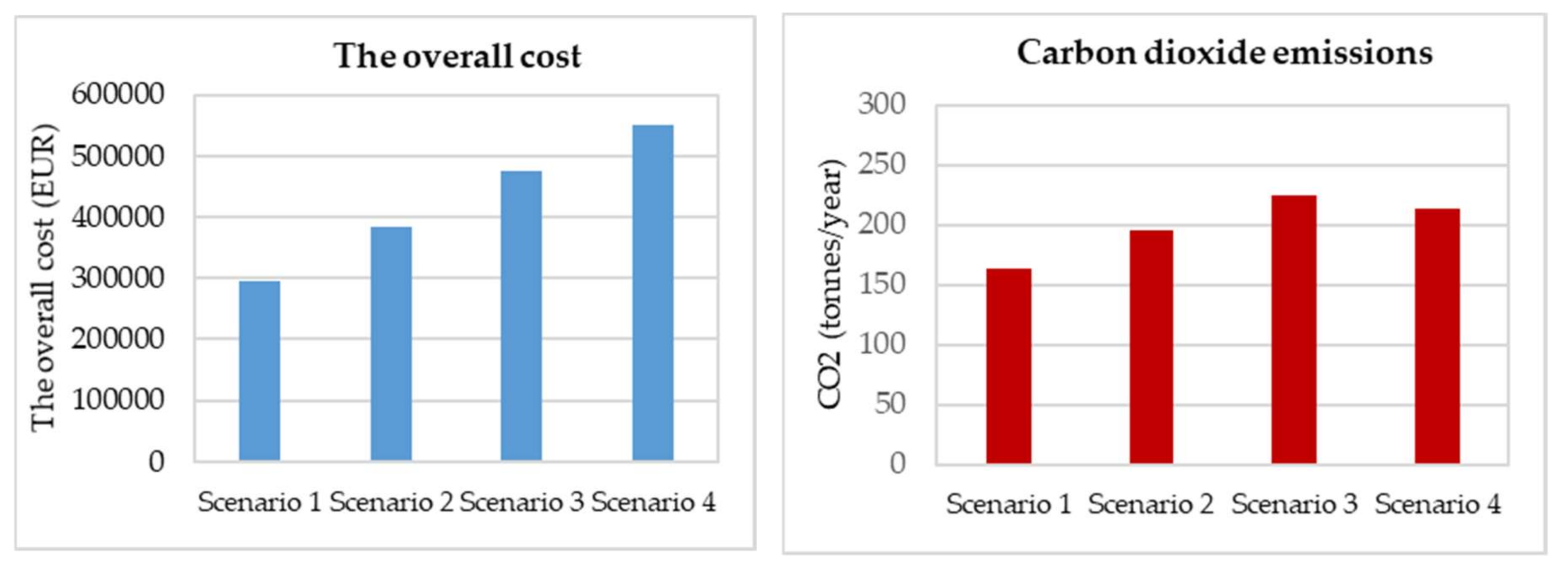
The overall costs (represented by the net present value) for each of the analysed scenarios are presented in
Table 6 and
Figure 8. Additionally, the carbon dioxide emissions are presented in
Figure 8. In terms of the load profiles of the analysed building, the minimum overall costs are observed in Scenario 1 and the maximum overall costs are observed in Scenario 4.
Out of the three forms of energy that are consumed in the building (electricity, heat, and cooling), the heat demand occupies the largest share of the total energy consumption of the building (see
Figure 3). Heat is required in both the HVAC system (heating, ventilation, and air conditioning) and the domestic hot water. Therefore, the energy sources that provide heat will have a major influence on the carbon dioxide emissions. Scenario 4 is considered to be the reference (traditional) scenario, in which heat and electricity are provided by public utility networks (the district heating system and the public electricity network). In Scenarios 1, 2, and 3, part of the energy that is required for the building is produced locally (including the energy that is produced by renewable energy sources). The carbon dioxide emissions are lower in Scenario 1 because of the heat pump, which provides a significant portion of the annual heat requirement. The carbon dioxide emissions are higher in Scenario 2 and Scenario 3 because of the heat that is generated by the boiler, even with the production of energy from renewable sources. It is clear that a larger production from renewable energy sources will lead to the reduction of the carbon dioxide emissions. However, such investments must be backed by support schemes.
One can notice that a new category of costs—namely the cost of carbon dioxide emissions—was included in the determination of the overall cost. These costs shall reflect the quantified, monetised, and discounted operational costs of CO2 that result from the carbon dioxide emissions—in tonnes of CO2 equivalent—over the calculation period.
The calculations that are required for selecting the energy sources according to the global costs have shown that there is significant potential for the achievement of cost-effective energy savings.
4. Conclusions
The energy audit of a building identifies refurbishment and upgrading solutions for the building to meet the minimum energy performance requirements. In the energy audit, both the envelope and the building's services are analysed. In the audit, the energy auditor recommends additional possible scenarios. Together with the building owner, the designer will choose the optimal solution package depending on the financial resources that are available, the legislative restrictions on the minimum energy performance requirements, and the environmental impact.
The refurbishment of existing buildings offers the possibility of an intervention to the building’s services in order to efficiently make use of the energy in the building. The energy sources for utilities and building services can be analysed in order to increase the energy performance of the building. The energy demand of the building is satisfied by means of specific energy carriers (heat, electricity, and cooling) for the building’s utilities, namely: heating, cooling, ventilation, domestic hot water, lighting, appliances, etc.
The selection of energy sources for the building’s utilities (heating, electricity, and cooling) was based on the concept of the energy hub. Through the use of this approach, various optimization issues with the use of energy in buildings can be identified.
In this paper, we analysed four scenarios. Scenario 4 is considered to be the reference (traditional) scenario. In this case, heat and electricity are provided by public utility networks (the district heating system and the public electricity network). Scenarios 1, 2, and 3 resulted from the selection of various energy sources that are available in the location of the building. The consideration of the carbon dioxide emissions penalties (the cost of carbon dioxide emissions) or the support schemes may lead to more favourable alternative solutions as opposed to the traditional scenario (heat and electricity provided by public utility networks). Thus, the renewable energy sources can occupy a growing share of the total energy consumption of the building.
When there are numerous ways to produce the same form of energy, various optimization issues can be identified in the operation of the building's services—considering that energy demands are not constant throughout the year.
The results that were obtained characterize the load profiles of the building under consideration. It is evident that the energy demands can be fulfilled by the selection of various energy sources that are available in the building’s location. These energy sources can be renewable energy sources (e.g., biomass, biogas, solar energy, geothermal energy, and wind energy) or public utility networks (natural gas, the district heating system, and the public electricity network). A higher share of renewable energy sources—while keeping the overall costs as low as possible—should be the target in the selection of energy sources.
When selecting energy sources, restrictions on the production of energy from renewable sources and the carbon dioxide emissions penalties should be considered.
The overall costs associated with meeting the minimum energy performance requirements (investment costs, maintenance and operating costs, costs of carbon dioxide emissions, and legislative restrictions on the production of energy from renewable sources) must be minimized over the estimated lifetime of the building. The proposed algorithm can also be used for new buildings. A joint examination of the energy sources and various technologies for the building’s services will demonstrate the effectiveness of the method that is used.


