
Research on Optimal Oil Filling Control Strategy of Wet Clutch in Agricultural Machinery

1
College of Engineering, Nanjing Agricultural University, Nanjing 210031, China
2
State Key Laboratory of Power System of Tractor, Luoyang 470139, China
3
Department of Vehicle Engineering, Nanjing Forestry University, Nanjing 210037, China
*
Author to whom correspondence should be addressed.
Actuators 2022, 11(11), 315; https://doi.org/10.3390/act11110315
Submission received: 19 September 2022
/
Revised: 21 October 2022
/
Accepted: 27 October 2022
/
Published: 30 October 2022
(This article belongs to the Section Actuators for Land Transport)
Abstract
:To improve the wet clutch engagement quality, which is widely used in agricultural machinery, the oil filling control strategy of a wet clutch is studied based on the method of simulation and experiment in detail in this paper. Firstly, this paper carries out the dynamic analysis of the wet clutch engagement process, establishes the mathematical model of the mechanical domain and the hydraulic domain of the hydraulic execution system, and designs the backstepping oil pressure controller. The controllability of the output oil pressure of the clutch hydraulic actuator is verified on the joint simulation platform of Matlab/Simulink (Version R2017b, MathWorks, Natick, MA, USA) and AMESim (Version 2019.1, Simcenter Amesim, Siemens Digital Industries Softwares, Berlin&Munuch, Germany). Then, this paper analyzes the clutch engagement process, extracts five factors affecting the oil filling process, and selects four clutch engagement quality evaluation indexes. An amount of 50 groups of experiments are carried out on the wet clutch oil filling test simulation platform built by SimulationX (Version 3.8, ESI ITI GmbH, Dresden, Germany). The response surface method (RSM) and stepwise regression analysis method are used to explore the mathematical models of the quality evaluation index and influencing factors of the oil filling process. Through 15 groups of random tests, the prediction accuracy of the stepwise regression model and the RSM model of each index is compared, and the models with high accuracy are selected to establish the comprehensive prediction mathematical model of clutch engagement quality, combined with the variance weight method. Finally, according to the working condition of the 3 MPa oil filling pressure studied in this paper, the optimal oil filling control strategy is obtained by the proposed clutch engagement quality prediction model. Under the target condition, when the oil filling rate of stage 1 is the highest and the proportion of phase 1’s duration to the total oil filling time is 69.65%, the oil filling rate of stage 2 is the lowest and the proportion of phase 2’s duration to the total oil filling time is 21.85%, and the proportion of phase 3’s duration to the total oil filling time is 8.51%, the engagement quality of wet clutch is the best. The research method of wet clutch optimal oil filling control strategy proposed in this paper provides a reliable method for the ride comfort research of agricultural machinery and clutch control.
1. Introduction
The wet clutch consists of friction disks (driving parts) and separate disks (driven parts). During the engagement process, the wet clutch transmits the torque by the friction between disks [1,2,3]. The wet clutch is widely used in agricultural equipment because of its smooth engagement and large torque transmission. The PST (power shift gearbox) relies on the sliding friction of a wet clutch to achieve the shift process without interruption, effectively improving the efficiency of agricultural machinery operations [4,5]. To realize tractor commutation without power interruption by switching forward and backward wet clutch, reducing the complexity of the drivers’ operation is required [6]. In HMCVT (hydraulic mechanical continuously variable transmission), the impact is reduced and the shift quality is improved by reasonably controlling multiple wet clutches [7]. As a key component, the dynamic engagement characteristics of the wet clutch will directly affect the performance of agricultural equipment. The wet clutch relies on hydraulic oil to combine. It is of great significance to study the oil-filling characteristics of the wet clutch to improve the clutch engagement quality.
The engagement pressure and engagement speed of the wet clutch are controlled by the hydraulic system of the clutch, so the oil pressure characteristics of the clutch have an important influence on the engagement quality. Li et al. [8] studied the relationship between clutch oil filling flow and clutch boost characteristics and proposed a clutch pre-oil filling control method. Wu et al. [9] established the mathematical model of a wet clutch hydraulic system, analyzed the influence of the control signal on the oil filling characteristics, and obtained that the selection of time area with a slowly rising duty ratio directly determined the action time and effect of buffer. Meng et al. [10] established a clutch electro-hydraulic control model and proposed a feedforward–feedback control strategy, and the control parameters were optimized according to the oil temperature and engine load. Kong et al. [11] designed an adaptive sliding mode controller to control the piston position of the wet clutch. Compared with the boundary layer sliding mode controller, the adaptive sliding mode controller had smaller fluctuation and faster convergence speed. Xue et al. [12] obtained the optimal curve of clutch engagement pressure by establishing a quadratic comprehensive performance index function in the wet clutch engagement process. Zeng et al. [13] built a simulation model of wet clutch hydraulic execution system, proposed a feedforward and PID feedback control algorithm based on the model, and verified that its control effect was better than the PID control algorithm. Fu et al. [14] constructed a complete nonlinear dynamic model of a wet clutch actuator and designed a wet clutch pressure controller based on MFAPC with the aim of investigating clutch cylinder pressure. In summary, the current research mostly focuses on the design of the wet clutch hydraulic control system to achieve accurate control of the clutch piston oil pressure, but there are few studies on the oil filling process, and there is a lack of research on the oil filling control strategy of the wet clutch from the perspective of improving the clutch engagement quality.
Because of the above problems, this paper mainly studies the following four points: (1) the hydraulic control system of the wet clutch is established based on AMESim and Simulink software; (2) the controllability of wet clutch piston pressure is verified by PID and backstepping controllers; (3) five factors influencing the oil-filling control process of the wet clutch are extracted, and the mathematical model between clutch engagement quality evaluation index and control factors is established by the RSM test; (4) the optimal oil-filling control strategy is obtained with stepwise regression analysis. This paper’s research provides a reliable method for improving the smoothness of agricultural machinery and the control of the wet clutch.
2. Materials and Methods
2.1. Modeling of Wet Clutch Engagement Process
With the increase in oil pressure, the wet clutch will exist in three states:
- (1)
- When the wet clutch is sliding, the dynamic equation of the clutch is:
In the formula, is the input torque of the wet clutch; is the friction torque of the wet clutch; is the resistance torque of the clutch driven shaft; is the rotational inertia of the clutch input shaft; is the rotational inertia of the clutch driven shaft; is the rotational speed of the clutch input shaft; is the rotational speed of the clutch driven shaft.
The calculation formula of wet clutch transmission torque is:
In the formula, is sliding friction coefficient, and its value is related to the rotational speed difference; is the number of friction plates; is the outer diameter of the friction plates; is the inner diameter of the friction plates; is the outer diameter of the piston; is the inner diameter of the piston, is the effective force area of the piston, is the stiffness of the return spring, is the displacement of the piston, and is the initial compression of return spring.
- (2)
- When the wet clutch is fully engaged, the speed of the input end and the output end is equal, and the dynamic equation is:
- (3)
- When the wet clutch is completely separated (assuming that the friction force can be neglected in this state), the dynamic equation is:
2.2. Establishment of Wet Clutch Hydraulic Control Platform
The hydraulic control system of the wet clutch consists of three parts: the power source, the oil pressure regulator, and the clutch hydraulic chamber. Figure 1 is the structure diagram of the pressure proportional solenoid valve and the clutch hydraulic chamber. Its main components are the proportional solenoid, valve spool, valve body, return spring, channel, oil drain hole, oil inlet, and oil outlet. The valve spool divides the valve body into four hydraulic chambers. Chambers 1 and 4 are decompressing cavities, which are connected with pressure-regulating chamber 2 through channels 1 and 2. Chamber 3 is the pressure supply chamber connected with a constant pressure source. When the solenoid valve coil is not powered, the valve spool is in the leftmost position because of the return spring. The oil inlet is closed, and chamber 2 is connected to the oil drain hole. The oil outlet’s pressure is 0 MPa, and the wet clutch is not combined. When the solenoid valve coil is powered, the valve spool compresses the return spring and moves to the right, and the oil inlet is gradually opened. The oil flows into chamber 2 through an oil outlet, which makes the pressure of chamber 2 and the output pressure of the solenoid valve increase gradually. Therefore, the oil pressure in the wet clutch’s piston chamber increases, and the engagement of the wet clutch is promoted. As the solenoid valve’s output pressure increases gradually, the pressure in chamber 1 and chamber 4 also increases gradually. Due to the different areas of the two decompressing cavities, the forces acting on the pressure feedback cavities are also different. Finally, the electromagnetic force, the return spring force, and the force of the pressure feedback chamber on both sides are balanced, and the solenoid valve’s output pressure is stable.
For the pressure-proportional solenoid valve that has strong nonlinear properties, in order to simplify the system modeling, this paper makes three simplifications: ① to ignore the influence of oil leakage during valve movement; ② the pressure of chamber 1 and chamber 4 is approximately equal to the output pressure proportional solenoid valve; and ③ to ignore the volume of chamber 1 and chamber 4 and the flow of hydraulic oil [15,16].
The kinematic equations of pressure proportional solenoid valve spool are shown in Formula (5).
In which is the electromagnetic force caused by the powered solenoid valve coil (N), is the excitation current flowing through the solenoid valve coil (N/A), is the resultant force acting on chamber 1 and chamber 4 (N), is the proportion coefficient of electromagnetic force and the current of the solenoid valve coil (N/A), is the output pressure of the solenoid valve (pa), and are the force areas of the solenoid valve’s left and right sides (m2), is the mass of the valve spool (kg), is the displacement of the valve spool (m), is the damping coefficient of the valve spool (Ns/m), and is the stiffness of the return spring (N/m).
The flow balance equations of the pressure-proportional solenoid valve are:
In which is the flow rate of the solenoid valve’s oil inlet (L/min), is the flow rate of the solenoid valve’s oil drain hole (L/min), is the flow rate flowing from the solenoid valve into the wet clutch’s piston chamber (L/min), is the volume of the solenoid valve chamber (m3), is the bulk modulus of oil (indicating the ability of oil to resist compression), is the flow coefficient of the solenoid valve, is the diameter of the valve spool (m), is the density of the hydraulic oil (kg/m3), is the oil pressure of the solenoid valve’s stabilized supply source (pa), is the oil pressure of the tank which is connected to the oil drain hole (pa), is the length of the solenoid valve’s oil drain hole (m), and is the output pressure of the solenoid valve (pa).
The mathematical model of the pressure-proportional solenoid valve, obtained from formula (5) and (6), is as formula (7):
When a certain amount of hydraulic oil flows into the clutch piston chamber, the volume flow and dynamic oil pressure in the piston chamber can be expressed as:
is the effective force area of the piston, is the displacement of the piston, is the bulk modulus of oil (indicating the ability of oil to resist compression), is the output pressure of the solenoid valve (pa), and is the initial volume of the clutch piston chamber (m3).
Additionally, the dynamic model of the piston during clutch engagement is:
In the formula, is the reaction force of the piston under contact pressure, is the damping coefficient of the piston, and is the mass of the piston.
According to formulas (5) to (9), the hydraulic control simulation platform of the wet clutch is established based on AMESim software (Version 2019.1, Simcenter Amesim, Siemens Digital Industries Softwares, Berlin&Munuch, Germany), as shown in Figure 2.
2.3. Design of Wet Clutch Oil Filling Controller Based on Backstepping Algorithm
Based on the mathematical model of the pressure-proportional solenoid valve, this paper adopts the backstepping algorithm [17,18,19] to design the oil pressure following the controller of the wet clutch. The principle of backstepping is to split the research system into multiple subsystems with lower orders, and to design virtual controllers for each subsystem from the subsystem where the control variable is located to the end of the input subsystem, so that the subsystem is stable in the Lyapunov sense [20]. The obtained system control input is obtained by backstepping and recursion.
By dividing formula (8) into three subsystems, and by selecting three state variables, (, , ), let the state variable =, where is the velocity of the valve spool. The system control input is , and the state equation of the wet clutch hydraulic control system is as follows:
The design of the backstepping controller is divided into three steps. First, to realize oil pressure following control, which is to make the solenoid valve’s output pressure follow the ideal control curve, then , is the excepted value of . Let error1 be . At this time, the control target is converted into . When taking the Lyapunov function , then
According to Lyapunov stability theory, the system is stable when takes the virtual control value , , , and then .
To make , let error2 be , and take the Lyapunov function as . Thus:
According to the Lyapunov stability theory, the system is stable when takes the virtual control value , and , (then ).
To make , let error3 be , and take the Lyapunov function as . Thus:
According to the Lyapunov stability theory, the system is stable when the system control input satisfies formula (12): and , , (then ). Formula (14) is the control law of the system control input.
The co-simulation of Matlab/Simulink and AMESim is used to verify the control effect of the system input control law of formula (14) on the piston oil pressure. The controller in Figure 3 is the oil pressure controller obtained by formula (15).
2.4. Wet Clutch Oil Filling Characteristics Influence Factor Divisions and Smoothness Evaluation Indexes
- Phase 1: after the solenoid valve coil of the wet clutch is electrified, the pressure in the piston cavity begins to build, and the gap between the friction plate and the steel plate is eliminated.
- Phase 2: with the increase in piston oil pressure, the friction plates and steel plates are further pressed. At this time, the clutch relies on rough friction torque and viscous torque to transmit torque.
- Phase 3: the piston oil pressure rises to the set value to ensure that the wet clutch has a certain reserve torque. At this time, there is no relative speed between friction plates and steel plates.
- Phase 4: the piston oil pressure remains constant until the controller issues new instructions.
Through analysis, this study selected five factors that affect the oil-filling characteristics curve—the oil-filling rate of phase 1, the proportion of phase 1’s duration to the total oil filling time, the oil-filling rate of phase 2, the proportion of phase 2’s duration to the total oil filling time, and the proportion of phase 3’s duration to the total oil filling time—to explore the influence of different oil-filling control strategies on the engagement quality of the wet clutch. In this paper, dynamic load, sliding friction work, impact degree, and engagement time are selected to evaluate the engagement quality of the wet clutch, and the comprehensive evaluation index of engagement quality of the wet clutch is established [24,25,26].
Dynamic load refers to the ratio of the maximum transmission torque to the stable transmission torque, indicating the fluctuation degree of the torque transmitted by the wet clutch.
In the formula, is dynamic load, is the maximum transmission torque during the wet clutch engagement process (Nm), and is the stable transmission torque during the wet clutch engagement process (Nm).
Sliding friction work is the work generated by the friction torque of the wet clutch when sliding, and sliding means there is a relative speed between friction plates and steel plates of the wet clutch. The friction work will accelerate the wear of clutch friction plates and reduce the service life of the clutch.
In the formula, is the sliding friction work (J), is the friction torque of the wet clutch (Nm), is the rotation speed of the friction plates (rad/s), is the rotation speed of the steel plates (rad/s), is the sliding start time (s), and is the sliding end time (s).
Impact degree refers to the change rate of the tractor’s longitudinal acceleration; the greater the impact, the lower the smoothness and the driving comfort of the tractor.
In the formula, is the impact degree (m/s3) and is the speed of tractor (m/s).
The engagement time refers to the time when the wet clutch receives the engagement instruction until there is no rotational speed difference between the friction plates and the steel plates.
In the formula, is the full engagement time (s), is the time when the wet clutch actuator receives the combined instruction (s), and is the time when there does not exist a speed difference(s) between the friction plate and the steel plate.
2.5. Simulation Test Platform for Oil Filling Control Strategy of Wet Clutch
Due to the noise interference in a bench test, this paper studies the oil filling control strategy of the wet clutch based on SimulationX software (Version 3.8, ESI ITI GmbH, Dresden, Germany), taking one stage of a stepped gearbox as an example. The specific parameters of the wet clutch in the oil-filled test platform are shown in Table 1, and the simulation test platform is shown in Figure 4. The working condition of the test is that a certain type of tractor (8.5 t) runs on flat ground without hanging agricultural machinery, and the engine speed is 1070 r/min. To validate the simulation model, this paper conducts simulation tests and bench tests of eight operating conditions (clutch oil pressure is 0.5, 1, 1.7, 2.4, 3.1, 3.8, 4.3, and 4.8 MPa, respectively) and compares the results (Table 2). One should adjust the simulation platform to match the engine speed (1070 r/min) and load (85.17 Nm) of the bench (Figure 5) and record the speed fluctuation of the gearbox output shaft. The comparison results are shown in Table 1.
For these 8 conditions, the relative error between the simulation results and the test results of the maximum output speed of the gearbox is 5.3%, which verifies the correctness of the simulation model.
2.6. Experimental Design Based on RSM
In this paper, the central composite design (CCD) in response surface methodology (RSM) is selected to design the simulation test of clutch engagement quality [27,28], and the number of the test groups is 50 in total (Table 3 and Table 4). CCD has the advantages of flexible design and fewer test times, which are widely used in scientific experiments.
The RSM is based on the least squares regression method to fit the statistical model, to approximate the real functional relationship, and to describe the relationship between input and response scientifically. The model can optimize and predict the response.
The code value and the actual value of each factor can be selected when modeling. The items in the model established by the two methods are the same, but each parameter is different. The relationship between the factors (, , , , and ) and the response values (, , , , and ) is shown in formula (19) [29,30].
In the formula, is the oil filling rate of phase 1, is the proportion of phase 1’s duration to the total oil filling time, is the oil filling rate of phase 2, is the proportion of phase 2’s duration to the total oil filling time, is the proportion of phase 3’s duration to the total oil filling time, and is the variation from other sources that the model cannot explain.
The first-order or second-order Taylor expansion is used to approximate the function form of the model in a relatively small region. The second-order model is:
3. Results and Discussion
3.1. Verification of Wet Clutch Piston Oil Pressure Control Effect
To verify the control effect of the controller designed in Chapter 2.3 on the clutch piston oil pressure under different system inputs, this paper studies the square wave signal and sine signal as the oil pressure control target for verification. As shown in Figure 6 and Figure 7, the oil pressure on the clutch piston can be effectively tracked according to the target curve.
When the target value changes with a square wave signal (Figure 6a), the total simulation test time is 3 s. In the first stage, the target oil pressure is 2.165 MPa, and the time required for the controller to stabilize to the target value is 0.05 s. The maximum oil pressure overshoot in this process is 0.923 MPa. In the second stage, the target oil pressure is 1.627 MPa, and the time required for the controller to stabilize to the target value is 0.106 s. In this process, the maximum oil pressure overshoot is 0.091 MPa. In the third stage, the target oil pressure is 1.075 MPa, and the time required for the controller to stabilize to the target value is 0.144 s. In this process, the maximum oil pressure overshoot is 0.102 MPa. Figure 6b is the error between the actual oil pressure and the target value in the process of oil pressure following control. The maximum following error of the first stage is 2.165 MPa, the maximum following error of the second stage is 0.538 MPa, and the maximum following error of the third stage is 0.552 MPa. When the target value of the wet clutch’s oil filling pressure changes with the sine signal (Figure 7), the total simulation test time is 3 s, the controller response time is 0.1 s, the following error is less than 0.01 MPa, and the maximum overshoot oil pressure is 0.026 MPa in the process of oil pressure following.
The simulation results show that the piston oil pressure controller, based on the backstepping algorithm, can achieve a better tracking effect to control the wet clutch with different oil filling characteristics curves.
At the same time, in order to further verify the control effect of the oil pressure controller designed in this paper, taking the square as an example, the backstepping controller is compared with the PID controller, which is commonly used in engineering. As shown in Figure 8, the final stable value of the square wave signal is 1.165 MPa. The PID controller oscillates violently within 0–0.099 s, and the overshoot of the backstepping controller is reduced by 78% compared with that of the PID controller. The backstepping controller is slower to stabilize to the expected value, but both controllers can quickly change to the expected value, and the required times are 0.099 s and 0.189 s, respectively.
The overshoot of the backstepping controller is relatively small, and the fluctuation of oil filling pressure is small. In the process of the wet clutch engagement, the fluctuation degree of oil filling pressure will directly affect the value of the wet clutch’s sliding friction work, which will aggravate the wear of the wet clutch in the long term and affect the service life and engagement quality.
3.2. Analysis of RSM Test Results
3.2.1. Analysis of Dynamic Load RSM Modeling Results
According to simulation test results of wet clutch engagement quality in Table 4, a quadratic regression polynomial model with dynamic load as a response value is established:
In the formula, is the oil filling rate of phase 1, is the proportion of phase 1’s duration to the total oil filling time, is the oil filling rate of phase 2, is the proportion of phase 2’s duration to the total oil filling time, is the proportion of phase 3’s duration to the total oil filling time, and is the dynamic load. Variance analysis of each model’s item is carried out to test the significance, and the results are shown in Table 5.
It can be seen from Table 5 that the p-value of the dynamic load regression model is less than 0.0001, indicating that the regression model is highly significant. Therefore, the model fitting accuracy is high and can be used to describe the sample. The fitting coefficient of the dynamic load regression model is 0.8792, the coefficient of adjustment is 0.7959, and the coefficient of variation is 6.29%. In summary, the regression model has high fitting accuracy, which can reflect the relationship between the five influencing factors and the dynamic load and can analyze and predict the dynamic load accurately.
In the variance analysis of the model, the influence of one-degree items A and B are significant (p < 0.05), and the significant degree of the five factors from high to low is A > B > D > C > E. B2 is the signature item in the second-order items (p < 0.05), indicating that the influence of factor B on dynamic load is nonlinear. In the cross items, AC and AD are significant (p < 0.05), indicating that there is a significant interaction between factor A and factor C, as well as factor A and factor D.
Figure 9 shows a curved surface, indicating that the influence of the interaction between factors A and C on the dynamic load is nonlinear. With the increase of the oil filling rate of phase 1 and the oil filling rate of phase 2, the dynamic load value increases gradually.
3.2.2. Analysis of Sliding Friction Work RSM Modeling Results
According to simulation test results of wet clutch engagement quality in Table 4, a quadratic regression polynomial model with sliding friction work as a response value is established:
It can be found from Table 6 that the p-value of the sliding friction work regression model is less than 0.0001, indicating that the regression model is highly significant. Therefore, the model fitting accuracy is high, and can be used to describe the sample. The fitting coefficient of the model is 0.9656, the coefficient of adjustment is 0.9504, and the coefficient of variation is 3.95%. In summary, the model has high fitting accuracy, which can reflect the relationship between the five influencing factors and the sliding friction work and can analyze and predict the sliding friction work accurately.
In the variance analysis of the sliding friction work regression model, the influence of the cross items AB, AC, and BC are significant (p < 0.05), indicating that there is a significant interaction between factor A and factor B, factor A and factor C, and factor B and factor C.
Figure 10 is almost a plane, indicating that the interaction between factors A and B has a linear effect on the sliding friction work. When the oil filling rate of phase 1 is constant, the value of the sliding friction work decreases with the increase in the proportion of phase 1’s duration to the total oil filling time.
3.2.3. Analysis of Impact Degree RSM Modeling Results
According to simulation test results of wet clutch engagement quality in Table 4, a quadratic regression polynomial model with impact degree as a response value is established. Variance analysis of each model’s item is carried out to test the significance. The results are shown in Table 7.
It can be seen from Table 7 that the p-value of the impact degree regression model is less than 0.0001, indicating that the regression model is highly significant. Therefore, the model fitting accuracy is high, and can be used to describe the sample. The fitting coefficient of the dynamic load regression model is 0.9047, the coefficient of adjustment is 0.8390, and the coefficient of variation is 9.89%. In summary, the regression model has high fitting accuracy, which can reflect the relationship between the five influencing factors and the impact degree and can analyze and predict the impact degree accurately.
In the variance analysis of the model, the influence of one-degree item A is significant (p < 0.05). In the second order items, A2, B2, and C2 are significant, indicating that the influence of factors A, B, and C on dynamic load is nonlinear. In the cross items, AB and AC are significant (p < 0.05), indicating that there is a significant interaction between factor A and factor B, as well as factor A and factor C.
The response surface in Figure 11 has a certain degree of bending. It indicates that the interaction between the oil filling rate of phase 1 and the proportion of phase 1’s duration to the total oil filling time has a linear effect on impact degree. When the oil filling rate of phase 1 is small and the proportion of phase 1’s duration to the total oil filling time is large, the impact degree is small.
3.2.4. Analysis of Engagement Time RSM Modeling Results
According to simulation test results of wet clutch engagement quality in Table 4, a quadratic regression polynomial model with full engagement time
as a response value is established. Variance analysis of each model’s item is carried out to test the significance. The results are shown in Table 8.
It can be found from Table 8 that the p-value of the impact degree regression model is less than 0.05, indicating that the regression model is highly significant. Therefore, the model fitting accuracy is high, and can be used to describe the sample. The fitting coefficient of the dynamic load regression model is 0.9832, the coefficient of adjustment is 0.9758, and the coefficient of variation is 4.50%. In summary, the regression model has high fitting accuracy, which can reflect the relationship between the five influencing factors and the full engagement time and can analyze and predict the full engagement time accurately.
In the variance analysis of the model, the influence of one degree item E is significant (p < 0.05). In the cross items, AB, AE, and DE are significant (p < 0.05), indicating that there is a significant interaction between factor A and factor B, factor A and factor E, and factor D and factor E.
Figure 12 is almost a plane. It indicates that the interaction between the oil filling rate of phase 1 and the proportion of phase 1’s duration to the total oil filling time has a linear effect on full engagement time. When the proportion of phase 1’s duration to the total oil filling time is constant, the value of full engagement time gradually decreases with the increase of the oil filling rate of phase 1.
3.3. Comparison of Two Modelling Method
To improve the model accuracy and simplify the model, this paper uses the stepwise regression method [31,32] to model the simulation test data in Table 4 and compares the prediction accuracy of the two methods. The regression models of the four evaluation indexes established by the stepwise regression method are shown in formulas 26–29:
The fitting coefficient of the dynamic load’s stepwise regression model is 0.847, and the coefficient of adjustment is 0.826. The fitting coefficient of the sliding friction work’s stepwise regression model is 0.960, and the coefficient of adjustment is 0.955. The fitting coefficient of the impact degree’s stepwise regression model is 0.877, and the coefficient of adjustment is 0.859. The fitting coefficient of the full engagement time’s stepwise regression model is 0.978, and the coefficient of adjustment is 0.975.
At the same time, 15 trials are randomly carried out to compare the prediction accuracy of RSM and stepwise regression model. The results are shown in Table 9.
By comparing the prediction accuracy of the stepwise regression model, it is shown that dynamic load, sliding friction work, impact degree, and full engagement time are higher than that of the RSM model. The prediction accuracy of the RSM model for impact degree is higher than the stepwise regression model. Therefore, the stepwise regression model is used to predict the dynamic load, sliding friction work, and full engagement time of the wet clutch during oil filling. The RSM model is used to predict the impact degree.
3.4. Optimal Oil Filling Control Strategy
To obtain the optimal oil-filling control strategy, this paper selects the variance weight method [33] to establish the comprehensive evaluation index of the wet clutch (Table 1) oil-filling process. After calculation, the weight of the dynamic load (w1) is 0.1516, the weight of the sliding friction work (w2) is 0.3146, the weight of the impact degree (w3) is 0.2997, and the weight of the full engagement time (w4) is 0.2341. By combining (26), (27), (28), and (29), the mathematical model of the comprehensive evaluation index of the wet clutch oil filling process is shown to be:
For the wet clutch in Table 1, when the oil filling pressure is 3 MPa, the optimal oil filling control strategy is determined according to the mathematical model of the comprehensive evaluation index of the oil filling process, as shown in Figure 13 (A = 75°, B = 69.65%, C = 15°, D = 21.85%, and E = 8.51%). Compared with the 50 groups of control strategies in Table 4, the clutch engagement quality of the oil-filling control strategy in Figure 13 is the best, and the comprehensive evaluation value is .
4. Conclusions
In this paper, the wet clutch, which is widely used in agricultural machinery, is taken as the research object. From the aspect of improving the engagement quality of the wet clutch, the oil-filling control strategy of the clutch is studied.
(1) The clutch oil pressure controller is established by the dynamic model of the wet clutch engagement process, and the controllability of the output oil pressure of the clutch hydraulic actuator is verified. Comparing the control effect of the backstepping oil pressure controller and the PID oil pressure controller, the overshoot generated in the control process of the former is smaller.
(2) For the wet clutch in Table 1, the stepwise regression model and RSM model between the four engagement quality evaluation indexes and the oil filling control strategy are compared. After comparison, it was found that the model prediction accuracy of dynamic load, sliding friction work, and engagement time using the stepwise regression method is higher, which corresponds to values of 91.23%, 96.29%, and 94.72%, respectively. The RSM model of impact degree has higher prediction accuracy. Through the variance weight analysis method, it was determined that, in the comprehensive evaluation index of engagement quality, the weight of the dynamic load is 0.1516, the weight of sliding friction work is 0.3146, the weight of impact degree is 0.2997, and the weight of engagement time is 0.2341.
(3) In this paper, the oil filling pressure of 3 MPa is taken as the research condition, and the optimal oil filling control strategy is obtained by the proposed clutch engagement quality prediction model. Under the target condition, when the oil filling rate of phase 1 is the highest and the proportion of phase 1’s duration to the total oil filling time is 69.65%, the oil filling rate of phase 2 is the lowest and the proportion of phase 2’s duration to the total oil filling time is 21.85%, and the proportion of phase 3’s duration to the total oil filling time is 8.51%, the wet clutch engagement quality is the best. The research method of wet clutch optimal oil filling control strategy proposed in this paper can provide a reliable method for the ride comfort research of agricultural machinery and the clutch control.
Author Contributions
Methodology, Y.Q. and Z.C.; software, Y.Q. and Z.C.; validation, Y.Q. and Z.C.; investigation, Y.Q., X.W. and Y.Z.; resources, Z.L. and L.W.; writing—original draft preparation, Y.Q.; writing—review and editing, Y.Q. and Z.L.; supervision, Z.L.; and project administration, Z.L. and Y.Q. All authors have read and agreed to the published version of the manuscript.
Funding
This research was funded by the National Key Research and Development Plan (2016YFD0701103), the Open Project of State Key Laboratory of Tractor Power System in China (SKT2022006), and the Postgraduate Research & Practice Program of Jiangsu Province (KYCX21_0572).
Data Availability Statement
The data presented in this study are available on demand from the corresponding author or first author at ([email protected] or [email protected]).
Acknowledgments
The authors thank the National Key Research and Development Plan (2016YFD0701103), the Open Project of State Key Laboratory of Tractor Power System in China (SKT2022006), and the Postgraduate Research & Practice Program of Jiangsu Province (KYCX21_0572) for funding. We also thank the anonymous reviewers for providing critical comments and suggestions that improved the manuscript.
Conflicts of Interest
The authors declare no conflict of interest.
References
- Xue, J.Q.; Ma, B.; Chen, M.; Zhang, Q.Q.; Zheng, L.J. Experimental Investigation and Fault Diagnosis for Buckled Wet Clutch Based on Multi-Speed Hilbert Spectrum Entropy. Entropy 2021, 23, 1704. [Google Scholar] [CrossRef] [PubMed]
- Jen, T.C.; Nemecek, D.J. Thermal analysis of a wet-disk clutch subjected to a constant energy engagement. Int. J. Heat Mass Transf. 2008, 51, 1757–1769. [Google Scholar] [CrossRef]
- Balan, A.E.; Caruntu, C.F.; Lazar, C. Simulation and control of an electro-hydraulic actuated clutch. Mech. Syst. Signal Process. 2011, 25, 1911–1922. [Google Scholar]
- Han, H.W.; Han, J.S.; Chung, W.J.; Kim, J.T.; Park, Y.J. Prediction of synchronization time for tractor power-shift transmission using multi-body dynamic simulation. Trans. ASABE 2021, 64, 1483–1498. [Google Scholar] [CrossRef]
- Wu, Y.W.; Yan, X.H.; Zhou, Z.L. Architecture modeling and test of tractor power shift transmission. IEEE Access 2021, 9, 3517–3525. [Google Scholar]
- Chen, X.D. Dynamic Control of Tractor Power-Shifting and Power-Reversing Process; Chongqing University: Chongqing, China, 2019. [Google Scholar]
- Wang, G.M.; Zhu, S.H.; Shi, L.X.; Tao, H.L.; Ruan, W.S. Experimental optimization on shift control of hydraulic mechanical continuously variable transmission for tractor. Trans. Chin. Soc. Agric. Eng. 2013, 29, 51–59. [Google Scholar]
- Li, Y.Y.; Liu, Y.J.; Chen, M. Wet clutch oiling control response characteristics analysis. Mach. Tool Hydraul. 2022, 50, 184–189. [Google Scholar]
- Wu, J.P.; Wang, L.Y.; Li, L.; Zhou, Q.J. The study on the influence of control signal on charge characteristics of wet clutch. Chin. Hydraul. Pneum. 2016, 2, 62–66. [Google Scholar]
- Meng, F.; Chen, H.Y.; Zhang, T.; Zhu, X.Y. Clutch fill control of an automatic transmission for heavy-duty vehicle applications. Mech. Syst. Signal Process. 2015, 64–65, 16–28. [Google Scholar] [CrossRef]
- Kong, H.F.; Du, D.W. Research on adaptive sliding mode control based on DCT clutch engagement process. J. Hefei Univ. Technol. 2019, 42, 721–726. [Google Scholar]
- Xue, D.L.; Feng, X.W.; Zheng, Z.L.; Cao, C. The fuzzy self-adaptive PID control of CVT’S multiple wet clutch based on the optimal pressure. Automot. Eng. 2019, 5, 424–428. [Google Scholar]
- Zeng, X.H.; Chen, H.X.; Dong, B.B.; Song, D.F. Modeling and Simulation of the Hydraulic Actuator System of Wet Clutch. Mach. Tool Hydraul. 2021, 49, 120–125. [Google Scholar]
- Fu, S.H.; Yang, Z.H.; Du, Y.F.; Li, Z.; Mao, E.R.; Zhu, Z.X. Starting control method for power shift tractor employing time-varying disturbance rejection. Trans. Chin. Soc. Agric. Mach. 2021, 52, 371–380. [Google Scholar]
- Meng, F.; Tao, G.; Chen, H.Y. A study on the dynamic response characteristics of electro-hydraulic proportional valve for the shift of automatic transmission. Automot. Eng. 2013, 45, 229–233. [Google Scholar]
- Yang, H.Y.; Shi, H.; Gong, G.F.; Hu, G.L. Electro-hydraulic proportional control of thrust system for shield tunneling machine. Autom. Constr. 2009, 18, 950–956. [Google Scholar]
- Wei, H.; Jin, X.H.; Huang, H.; Tao, P. Backstepping control for electro-hydraulic force-loading system with position disturbance. J. Wuhan Univ. Sci. Technol. 2020, 43, 213–218. [Google Scholar]
- Fu, D.X.; Zhao, X.M. Backstepping terminal sliding mode position control based on neural network observer. Control. Theory Appl. 2022, 39, 690–707. [Google Scholar]
- Shi, Q.; Liu, X.; Ying, H.L.; Wang, M.Q.; He, Z.J.; He, L. Study on the backstepping control algorithm for the hydraulic process in electro-hydraulic brake-by-wire system. Automot. Eng. 2022, 44, 747–755. [Google Scholar]
- He, L.; Li, L.F.; Wei, Y.J.; He, Z.J.; Gao, B.Z.; Shi, Q. Backstepping control algorithm for steer-by-wire angle tracking. China J. Highw. Transp. 2021, 34, 51–60. [Google Scholar]
- Wang, C. Research on Starting Control of DCT Vehicle Considering Dynamic Engagement Characteristics of Wet Clutch; Chongqing University: Chongqing, China, 2020. [Google Scholar]
- Mason, R.L.; Gunst, R.F.; Hess, J.L. Statistical Design and Analysis of Experiments with Applications to Engineering and Science; John Wiley and Sons Publication: Hoboken, NJ, USA, 2020. [Google Scholar]
- Li, A.T.; Qin, D.T. Adaptive model predictive control of dual clutch transmission shift based on dynamic friction coefficient estimation. Mech. Mach. Theory 2022, 173, 104804. [Google Scholar] [CrossRef]
- Hu, H.W. Study on the Characteristic of Automatic wet Clutch Engagement Process; Zhejiang University: Hangzhou, China, 2008. [Google Scholar]
- Shang, X.B. Theoretical Analysis and Experiment Study on Engagement Process of wet Clutch; Zhejiang University: Hangzhou, China, 2019. [Google Scholar]
- Ma, B. Dynamic performance simulation of vehicular power shift clutch charge process. J. Beijing Inst. Technol. 2000, 2, 188–192. [Google Scholar]
- Abdi, M.R.; Ghalandarzadeh, A.; Shafiei-Chafi, L. Optimization of line and fiber content for improvement of clays with different plasticity using response surface method (RSM). Transp. Geotech. 2022, 32, 100685. [Google Scholar] [CrossRef]
- Cui, J.; Zhao, Z.H.; Liu, J.W.; Hu, P.X.; Zhou, R.N.; Ren, G.X. Uncertainty analysis of mechanical dynamics by combining response surface method with signal decomposition technique. Mech. Syst. Signal Process. 2021, 158, 107570. [Google Scholar] [CrossRef]
- Fang, J.T. Comparison for Experimental Designs and Modeling in Response Surface Methodology; Tianjin University: Tianjin, China, 2011. [Google Scholar]
- Li, L.; Zhang, S.; He, Q.; Hu, X.B. Application of Response Surface Methodology in Experiment Design and Optimization. Res. Explor. Lab. 2015, 34, 41–45. [Google Scholar]
- Qian, Y.; Cheng, Z.; Lu, Z.X. Study on stepwise optimization on shift quality of heavy-duty tractor HMCVT based on five tractors. J. Nanjing Agric. Univ. 2020, 43, 564–573. [Google Scholar]
- Zhang, Z.C.; Wang, H.F.; Han, W.X.; Bian, J.; Chen, S.B.; Cui, T. Inversion of moisture content based on multispectral remote sensing of UAVs. Trans. Chin. Soc. Agric. Mach. 2018, 49, 173–181. [Google Scholar]
- Qian, Y.; Cheng, Z.; Lu, Z.X. Bench Testing and Modeling Analysis of Optimum Shifting Point of HMCVT. Complexity 2021, 2021, 6629561. [Google Scholar] [CrossRef]
Figure 1.
Schematic diagram of the pressure-proportional solenoid valve.
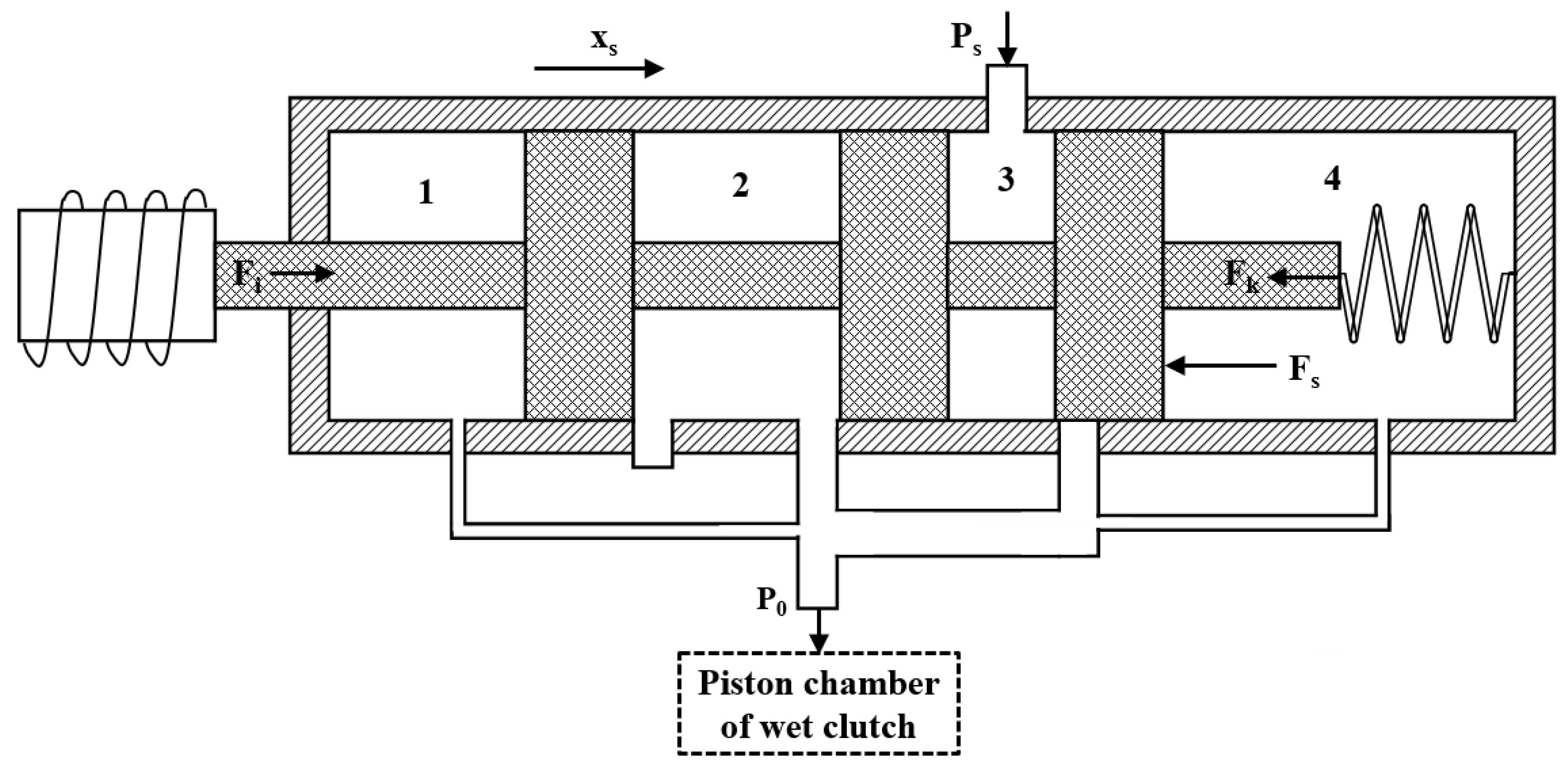
Figure 2.
The hydraulic control simulation platform of the wet clutch. The component in red is control signal, components in dark red are hydraulic bodies, components in green are mechanical components, components in dark green are friction plates.
Figure 2.
The hydraulic control simulation platform of the wet clutch. The component in red is control signal, components in dark red are hydraulic bodies, components in green are mechanical components, components in dark green are friction plates.

Figure 3.
The hydraulic control simulation platform based on formula (15) of the wet clutch.

Figure 4.
Simulation test platform for the oil filling control strategy of the wet clutch.

Figure 5.
Test bench to verify the simulation test platform based on SimulationX. It includes the: ① engine, ② transmission assembly, ③ pump–motor system, ④ rotating speed–torque sensor, ⑤ electric eddy current dynamometer, and ⑥ hydraulic control system.
Figure 5.
Test bench to verify the simulation test platform based on SimulationX. It includes the: ① engine, ② transmission assembly, ③ pump–motor system, ④ rotating speed–torque sensor, ⑤ electric eddy current dynamometer, and ⑥ hydraulic control system.

Figure 6.
Square wave signal following control of oil pressure controller based on the backstepping algorithm. (a) Target oil pressure; (b) following error.
Figure 6.
Square wave signal following control of oil pressure controller based on the backstepping algorithm. (a) Target oil pressure; (b) following error.

Figure 7.
Sine wave signal following control of oil pressure controller based on backstepping algorithm. (a) Target oil pressure; (b) following error.
Figure 7.
Sine wave signal following control of oil pressure controller based on backstepping algorithm. (a) Target oil pressure; (b) following error.

Figure 8.
Comparison of following control effect between the backstepping controller and the PID controller.
Figure 8.
Comparison of following control effect between the backstepping controller and the PID controller.

Figure 9.
Response surface diagram and contour map of factor A and C on interaction of dynamic load. (a) Response surface diagram; (b) contour map. The four contour lines mapped on the bottom of Figure 9a correspond to the four types of dynamic load in Figure 9b.

Figure 10.
Response surface diagram and contour map of factor A and B on interaction of sliding friction work. (a) Response surface diagram; (b) contour map. The four contour lines mapped on the bottom of Figure 10a correspond to the four types of sliding friction work in Figure 10b.

Figure 11.
Response surface diagram and contour map of factor A and B on interaction of impact degree. (a) Response surface diagram; (b) contour map. The three contour lines mapped on the bottom of Figure 11a correspond to the three types of impact degree in Figure 11b.

Figure 12.
Response surface diagram and contour map of factor A and B on interaction of full engagement time. (a) Response surface diagram; (b) contour map. The four contour lines mapped on the bottom of Figure 12a correspond to the four types of full engagement time in Figure 12b.

Figure 13.
Optimal oil filling control strategy for verification conditions.


Table 1.
Simulation Parameters of wet clutch oil filling test platform.
| Parameter | Value | Parameter | Value |
|---|---|---|---|
| Sticking friction coefficient | 0.12 | Slipping friction coefficient | 0.08 |
| Outer diameter of clutch friction plates (mm) | 135 | Number of clutch friction pairs | 8 |
| External diameter of clutch friction plates (mm) | 164 | The thickness of clutch friction plates | 3 |
Table 2.
Results comparison.
| Number | Bench Test Results (r/min) | Simulation Test Results (r/min) | Relative Error (%) | Average Relative Error (%) |
|---|---|---|---|---|
| 1 | 291 | 282.01 | 3.04 | 5.3 |
| 2 | 299.25 | 283.21 | 5.3 | |
| 3 | 306.25 | 284.17 | 7.2 | |
| 4 | 302.75 | 285.66 | 5.6 | |
| 5 | 303.25 | 286.64 | 5.5 | |
| 6 | 304.75 | 287.22 | 5.8 | |
| 7 | 304.25 | 287.78 | 5.4 | |
| 8 | 303.75 | 288.12 | 5.1 |
Table 3.
Factors and levels of RSM test.
| Factors | Levels | ||||
|---|---|---|---|---|---|
| A | 15° (−2) | 30° (−1) | 45° (0) | 60° (1) | 75° (2) |
| B | 10% (−2) | 15% (−1) | 20% (0) | 25% (1) | 30% (2) |
| C | 15° (−2) | 30° (−1) | 45° (0) | 60° (1) | 75° (2) |
| D | 10% (−2) | 15% (−1) | 20% (0) | 25% (1) | 30% (2) |
| E | 10% (−2) | 15% (−1) | 20% (0) | 25% (1) | 30% (2) |
Note: The code value in brackets corresponding to each level of each factor in RSM tests.
Table 4.
RSM test design and results of different oil filling curves on the wet clutch engagement quality.
Table 4.
RSM test design and results of different oil filling curves on the wet clutch engagement quality.
| Test Number | The Code Value of Factors | Evaluation Index of Wet Clutch Engagement Quality | |||||||
|---|---|---|---|---|---|---|---|---|---|
| A | B | C | D | E | y1 | y2 (J) | y3 (m/s3) | y4 (S) | |
| 1 | −1 | 1 | 1 | −1 | 1 | 3.3891 | 608.7464 | 18.0604 | 0.4475 |
| 2 | −1 | 1 | 1 | −1 | −1 | 3.3891 | 608.7464 | 18.2110 | 0.4475 |
| 3 | 0 | 0 | 0 | 0 | 0 | 3.0969 | 486.8665 | 16.2769 | 0.3275 |
| 4 | 0 | −2 | 0 | 0 | 0 | 3.1004 | 486.5006 | 16.7344 | 0.3222 |
| 5 | 0 | 2 | 0 | 0 | 0 | 3.0950 | 486.3843 | 18.1973 | 0.3289 |
| 6 | 1 | 1 | −1 | 1 | 1 | 3.7551 | 396.2355 | 25.9036 | 0.2277 |
| 7 | −1 | 1 | −1 | −1 | 1 | 2.5997 | 620.9123 | 12.2579 | 0.4658 |
| 8 | 0 | 0 | 2 | 0 | 0 | 3.6988 | 486.1870 | 20.4988 | 0.3183 |
| 9 | 1 | −1 | 1 | 1 | 1 | 3.7539 | 396.2330 | 22.0172 | 0.2263 |
| 10 | 0 | 0 | 0 | 0 | 0 | 3.0969 | 486.8635 | 16.2769 | 0.3261 |
| 11 | 1 | −1 | 1 | −1 | 1 | 3.7539 | 396.2330 | 22.4485 | 0.2263 |
| 12 | 1 | −1 | −1 | −1 | −1 | 3.7539 | 396.2330 | 22.0376 | 0.2263 |
| 13 | 0 | 0 | −2 | 0 | 0 | 2.9059 | 487.0966 | 15.5220 | 0.3246 |
| 14 | −2 | 0 | 0 | 0 | 0 | 3.0984 | 609.4035 | 17.1849 | 0.5345 |
| 15 | 0 | 0 | 0 | 0 | 0 | 3.0969 | 486.8484 | 16.4291 | 0.3227 |
| 16 | 1 | −1 | −1 | 1 | −1 | 3.7539 | 396.2330 | 21.6240 | 0.2263 |
| 17 | −1 | −1 | −1 | −1 | 1 | 3.0752 | 620.4315 | 14.9747 | 0.4699 |
| 18 | 1 | −1 | 1 | 1 | −1 | 3.7539 | 396.2330 | 22.2299 | 0.2263 |
| 19 | 1 | −1 | −1 | −1 | 1 | 3.7539 | 396.2330 | 21.8362 | 0.2263 |
| 20 | −1 | −1 | −1 | 1 | −1 | 3.7336 | 534.9278 | 20.7967 | 0.3808 |
| 21 | −1 | −1 | 1 | 1 | 1 | 4.3965 | 507.8907 | 29.7387 | 0.3555 |
| 22 | 1 | −1 | 1 | −1 | −1 | 3.7539 | 396.2330 | 22.4491 | 0.2263 |
| 23 | 0 | 0 | 0 | 0 | 0 | 3.0969 | 486.8665 | 16.2769 | 0.3275 |
| 24 | 0 | 0 | 0 | 0 | 2 | 3.0969 | 486.8665 | 16.1278 | 0.3275 |
| 25 | −1 | −1 | −1 | 1 | 1 | 2.6025 | 620.5252 | 13.2391 | 0.4654 |
| 26 | −1 | 1 | −1 | 1 | −1 | 2.5997 | 620.9123 | 12.1363 | 0.4658 |
| 27 | 1 | 1 | 1 | 1 | −1 | 3.7551 | 396.2325 | 27.1737 | 0.2264 |
| 28 | 1 | 1 | −1 | 1 | −1 | 3.7551 | 396.2325 | 26.6489 | 0.2264 |
| 29 | 0 | 0 | 0 | 0 | 0 | 3.0969 | 486.8433 | 16.4291 | 0.3202 |
| 30 | 0 | 0 | 0 | 0 | 0 | 3.0969 | 486.8665 | 16.4291 | 0.3275 |
| 31 | −1 | 1 | 1 | 1 | 1 | 3.3891 | 608.7451 | 17.5980 | 0.4462 |
| 32 | −1 | −1 | 1 | 1 | −1 | 3.7336 | 534.9278 | 20.4164 | 0.3808 |
| 33 | 1 | 1 | −1 | −1 | −1 | 3.7551 | 396.2325 | 25.8938 | 0.2264 |
| 34 | 1 | 1 | −1 | −1 | 1 | 3.7551 | 396.2325 | 26.1471 | 0.2264 |
| 35 | 0 | 0 | 0 | −2 | 0 | 3.0969 | 486.8433 | 16.2723 | 0.3202 |
| 36 | −1 | 1 | −1 | −1 | −1 | 2.5997 | 620.9123 | 12.3657 | 0.4658 |
| 37 | −1 | 1 | 1 | 1 | −1 | 3.3891 | 608.7272 | 17.7497 | 0.4414 |
| 38 | 0 | 0 | 0 | 2 | 0 | 3.0969 | 486.8433 | 15.9782 | 0.3202 |
| 39 | 1 | 1 | 1 | −1 | 1 | 3.7551 | 396.2235 | 28.5734 | 0.2244 |
| 40 | −1 | −1 | −1 | −1 | −1 | 3.3482 | 620.3871 | 17.3163 | 0.4652 |
| 41 | −1 | 1 | −1 | 1 | 1 | 2.5997 | 620.9123 | 12.9101 | 0.4658 |
| 42 | 1 | 1 | 1 | 1 | 1 | 3.7551 | 396.2325 | 28.8718 | 0.2264 |
| 43 | 0 | 0 | 0 | 0 | 0 | 3.0969 | 486.8433 | 16.9029 | 0.3202 |
| 44 | 0 | 0 | 0 | 0 | 0 | 3.0969 | 486.8665 | 16.9029 | 0.3275 |
| 45 | 2 | 0 | 0 | 0 | 0 | 5.0108 | 314.6145 | 29.2979 | 0.1461 |
| 46 | −1 | −1 | 1 | −1 | 1 | 3.7336 | 534.9278 | 21.4024 | 0.3808 |
| 47 | 1 | −1 | −1 | 1 | 1 | 3.7539 | 396.2330 | 22.7041 | 0.2263 |
| 48 | 1 | 1 | 1 | −1 | −1 | 3.7551 | 396.2325 | 27.9957 | 0.2264 |
| 49 | −1 | −1 | 1 | −1 | −1 | 3.7336 | 534.9278 | 20.9810 | 0.3808 |
| 50 | 0 | 0 | 0 | 0 | −2 | 3.0969 | 486.8433 | 16.5790 | 0.3202 |
Table 5.
Significance test of the dynamic load regression model.
| Source | Sum of Squares | df | Mean Square | F-Value | Prob > F | Result |
|---|---|---|---|---|---|---|
| Model | 9.72 | 20 | 0.49 | 10.55 | <0.0001 | significant |
| A | 9.72 | 20 | 0.49 | 10.55 | <0.0001 | |
| B | 0.22 | 1 | 0.22 | 4.79 | 0.0369 | |
| C | 0.016 | 1 | 0.016 | 0.35 | 0.5589 | |
| D | 0.10 | 1 | 0.10 | 2.25 | 0.1446 | |
| E | 3.494 × 10⁻³ | 1 | 3.494 × 10⁻³ | 0.076 | 0.7849 | |
| AB | 0.024 | 1 | 0.024 | 0.51 | 0.4789 | |
| AC | 0.61 | 1 | 0.61 | 13.21 | 0.0011 | |
| AD | 1.12 | 1 | 1.12 | 24.39 | <0.0001 | |
| AE | 0.010 | 1 | 0.010 | 0.22 | 0.6389 | |
| BC | 0.017 | 1 | 0.017 | 0.37 | 0.5462 | |
| BD | 3.196 × 10⁻³ | 1 | 3.196 × 10⁻³ | 0.069 | 0.7941 | |
| BE | 0.010 | 1 | 0.010 | 0.22 | 0.6389 | |
| CD | 0.017 | 1 | 0.017 | 0.37 | 0.5462 | |
| CE | 0.018 | 1 | 0.018 | 0.38 | 0.5414 | |
| DE | 0.13 | 1 | 0.13 | 2.90 | 0.0993 | |
| A2 | 1.191 × 10⁻³ | 1 | 1.191 × 10⁻³ | 0.026 | 0.8734 | |
| B2 | 2.23 | 1 | 2.23 | 48.53 | <0.0001 | |
| C2 | 0.020 | 1 | 0.020 | 0.44 | 0.5147 | |
| D2 | 0.19 | 1 | 0.19 | 4.03 | 0.0540 | |
| E2 | 0.020 | 1 | 0.020 | 0.43 | 0.5180 |
Table 6.
Significance test of the sliding friction work regression model.
| Source | Sum of Squares | df | Mean Square | F-Value | Prob > F | Result |
|---|---|---|---|---|---|---|
| Model | 3.575 × 10⁵ | 15 | 23,833.52 | 63.58 | <0.0001 | significant |
| A | 1374.87 | 1 | 1374.87 | 3.67 | 0.0639 | |
| B | 46.63 | 1 | 46.63 | 0.12 | 0.7265 | |
| C | 337.00 | 1 | 337.00 | 0.90 | 0.3497 | |
| D | 455.36 | 1 | 455.36 | 1.21 | 0.2781 | |
| E | 7.990 × 10⁻⁵ | 1 | 7.990 × 10⁻⁵ | 2.132 × 10⁻⁵ | 0.9996 | |
| AB | 5244.89 | 1 | 5244.89 | 13.99 | 0.0007 | |
| AC | 3450.10 | 1 | 3450.10 | 9.20 | 0.0046 | |
| AD | 395.05 | 1 | 395.05 | 1.05 | 0.3119 | |
| AE | 107.42 | 1 | 107.42 | 0.29 | 0.5959 | |
| BC | 1724.33 | 1 | 1724.33 | 4.60 | 0.0392 | |
| BD | 394.76 | 1 | 394.76 | 1.05 | 0.3120 | |
| BE | 107.28 | 1 | 107.28 | 0.29 | 0.5961 | |
| CD | 106.27 | 1 | 106.27 | 0.28 | 0.5979 | |
| CE | 396.73 | 1 | 396.73 | 1.06 | 0.3109 | |
| DE | 107.11 | 1 | 107.11 | 0.29 | 0.5964 |
Table 7.
Significance test of the impact degree regression model.
| Source | Sum of Squares | df | Mean Square | F-Value | Prob > F | Result |
|---|---|---|---|---|---|---|
| Model | 1053.59 | 20 | 52.68 | 13.77 | <0.0001 | significant |
| A | 52.12 | 1 | 52.12 | 13.62 | 0.0009 | |
| B | 7.62 | 1 | 7.62 | 1.99 | 0.1688 | |
| C | 6.96 | 1 | 6.96 | 1.82 | 0.1879 | |
| D | 2.28 | 1 | 2.28 | 0.60 | 0.4464 | |
| E | 6.76 | 1 | 6.76 | 1.77 | 0.1941 | |
| AB | 187.39 | 1 | 187.39 | 48.98 | <0.0001 | |
| AC | 48.01 | 1 | 48.01 | 12.55 | 0.0014 | |
| AD | 2.66 | 1 | 2.66 | 0.69 | 0.4113 | |
| AE | 0.16 | 1 | 0.16 | 0.041 | 0.8409 | |
| BC | 0.25 | 1 | 0.25 | 0.065 | 0.8009 | |
| BD | 3.02 | 1 | 3.02 | 0.79 | 0.3815 | |
| BE | 0.084 | 1 | 0.084 | 0.022 | 0.8834 | |
| CD | 0.20 | 1 | 0.20 | 0.053 | 0.8200 | |
| CE | 12.94 | 1 | 12.94 | 3.38 | 0.0761 | |
| DE | 1.04 | 1 | 1.04 | 0.27 | 0.6068 | |
| A2 | 150.60 | 1 | 150.60 | 39.36 | <0.0001 | |
| B2 | 16.84 | 1 | 16.84 | 4.40 | 0.0447 | |
| C2 | 23.76 | 1 | 23.76 | 6.21 | 0.0187 | |
| D2 | 4.88 | 1 | 4.88 | 1.27 | 0.2682 | |
| E2 | 6.40 | 1 | 6.40 | 1.67 | 0.2059 |
Table 8.
Significance test of the full engagement time regression model.
| Source | Sum of Squares | df | Mean Square | F-Value | Prob > F | Result |
|---|---|---|---|---|---|---|
| Model | 1.062 × 10⁻³ | 1 | 1.062 × 10⁻³ | 4.86 | 0.0343 | significant |
| A | 4.081 × 10⁻⁵ | 1 | 4.081 × 10⁻⁵ | 0.19 | 0.6682 | |
| B | 2.115 × 10⁻⁴ | 1 | 2.115 × 10⁻⁴ | 0.97 | 0.3320 | |
| C | 4.656 × 10⁻⁴ | 1 | 4.656 × 10⁻⁴ | 2.13 | 0.1534 | |
| D | 1.286 × 10⁻⁷ | 1 | 1.286 × 10⁻⁷ | 5.891 × 10⁻⁴ | 0.9808 | |
| E | 4.198 × 10⁻³ | 1 | 4.198 × 10⁻³ | 19.23 | 0.0001 | |
| AB | 4.073 × 10⁻³ | 1 | 4.073 × 10⁻³ | 18.65 | 0.0001 | |
| AC | 4.879 × 10⁻⁴ | 1 | 4.879 × 10⁻⁴ | 2.23 | 0.1442 | |
| AD | 1.509 × 10⁻⁴ | 1 | 1.509 × 10⁻⁴ | 0.69 | 0.4116 | |
| AE | 1.240 × 10⁻³ | 1 | 1.240 × 10⁻³ | 5.68 | 0.0229 | |
| BC | 3.799 × 10⁻⁴ | 1 | 3.799 × 10⁻⁴ | 1.74 | 0.1960 | |
| BD | 1.122 × 10⁻⁴ | 1 | 1.122 × 10⁻⁴ | 0.51 | 0.4784 | |
| BE | 1.019 × 10⁻⁴ | 1 | 1.019 × 10⁻⁴ | 0.47 | 0.4991 | |
| CD | 3.994 × 10⁻⁴ | 1 | 3.994 × 10⁻⁴ | 1.83 | 0.1851 | |
| CE | 1.225 × 10⁻⁴ | 1 | 1.225 × 10⁻⁴ | 0.56 | 0.4589 | |
| DE | 1.062 × 10⁻³ | 1 | 1.062 × 10⁻³ | 4.86 | 0.0343 |
Table 9.
Comparison of prediction accuracy between the RSM models and the stepwise models.
| Evaluation Index | Prediction Accuracy (%) | |
|---|---|---|
| RSM | Stepwise Regression Method | |
| Dynamic load Sliding friction work (J) | 90.90 | 91.23 |
| 94.25 | 96.29 | |
| Impact degree (m/s3) | 76.73 | 38.63 |
| Full engagement time (s) | 92.16 | 94.72 |
Publisher’s Note: MDPI stays neutral with regard to jurisdictional claims in published maps and institutional affiliations. |
© 2022 by the authors. Licensee MDPI, Basel, Switzerland. This article is an open access article distributed under the terms and conditions of the Creative Commons Attribution (CC BY) license (https://creativecommons.org/licenses/by/4.0/).
Share and Cite
MDPI and ACS Style
Qian, Y.; Wang, L.; Cheng, Z.; Zhao, Y.; Wang, X.; Lu, Z. Research on Optimal Oil Filling Control Strategy of Wet Clutch in Agricultural Machinery. Actuators 2022, 11, 315. https://doi.org/10.3390/act11110315
AMA Style
Qian Y, Wang L, Cheng Z, Zhao Y, Wang X, Lu Z. Research on Optimal Oil Filling Control Strategy of Wet Clutch in Agricultural Machinery. Actuators. 2022; 11(11):315. https://doi.org/10.3390/act11110315
Chicago/Turabian StyleQian, Yu, Lin Wang, Zhun Cheng, Yirong Zhao, Xingwei Wang, and Zhixiong Lu. 2022. "Research on Optimal Oil Filling Control Strategy of Wet Clutch in Agricultural Machinery" Actuators 11, no. 11: 315. https://doi.org/10.3390/act11110315
Note that from the first issue of 2016, this journal uses article numbers instead of page numbers. See further details here.