
Control Allocation Design for Torpedo-Like Underwater Vehicles with Multiple Actuators

Abstract
:1. Introduction
2. Mathematical Model and the Desired Control Law for Torpedo-Like Underwater Vehicles
2.1. Problem Formulation
2.1.1. Dynamics of Underwater Vehicle and Robust Control Law
2.1.2. Control Allocation Design
2.2. Actuator Models
3. Control Allocation Methods for Torpedo-Like Underwater Vehicles
Least Squares Optimization Method
4. Implementation for a Torpedo-Like Underwater Vehicle
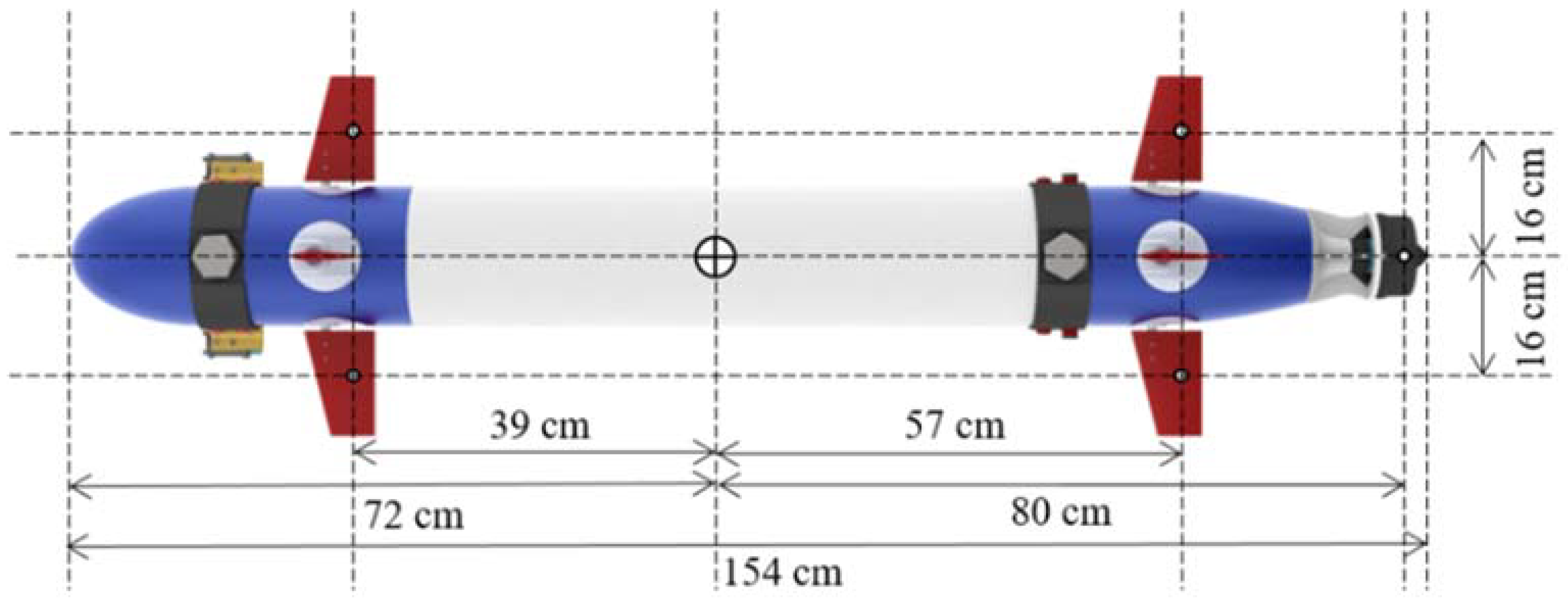
4.1. The Specifications of the Underwater Vehicle
4.2. The Configuration Matrix of the Torpedo-Like Underwater Vehicle
4.3. The Actuator Model of the Underwater Vehicle
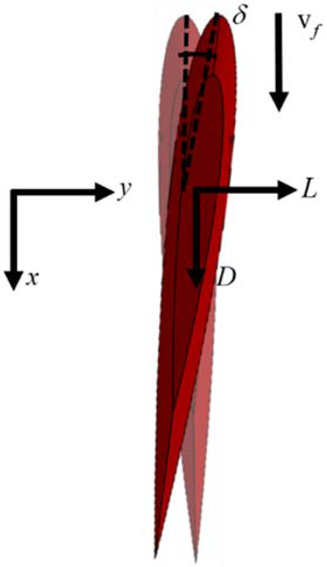
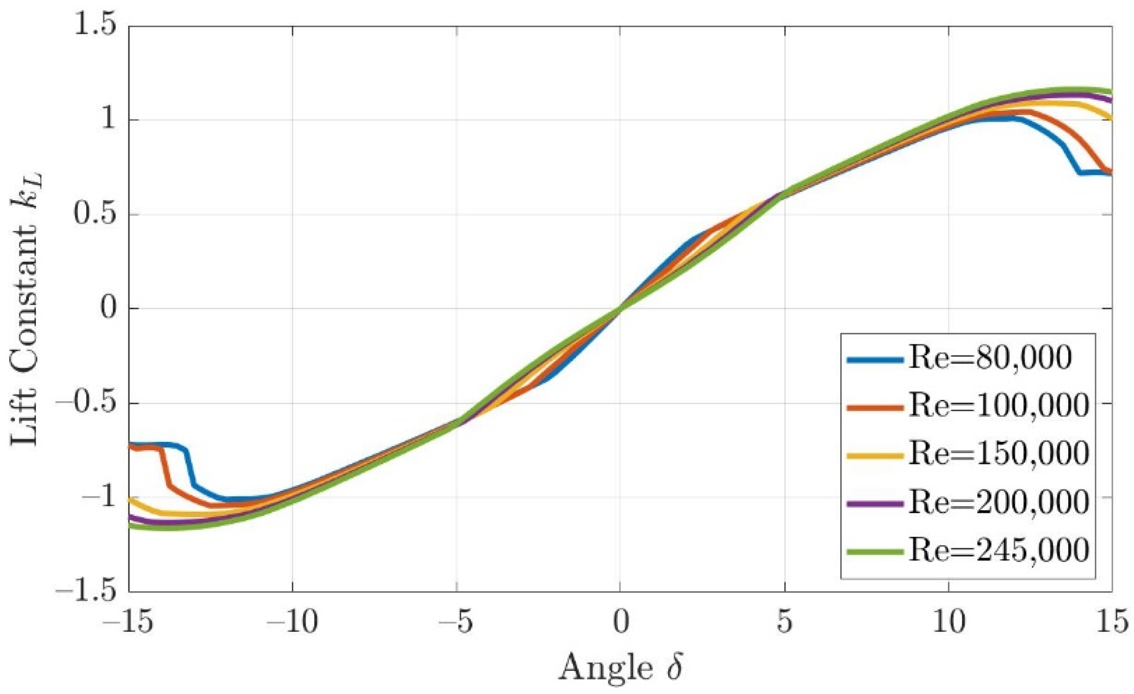
4.3.1. The Hydrodynamics Model of Fins and Rudders
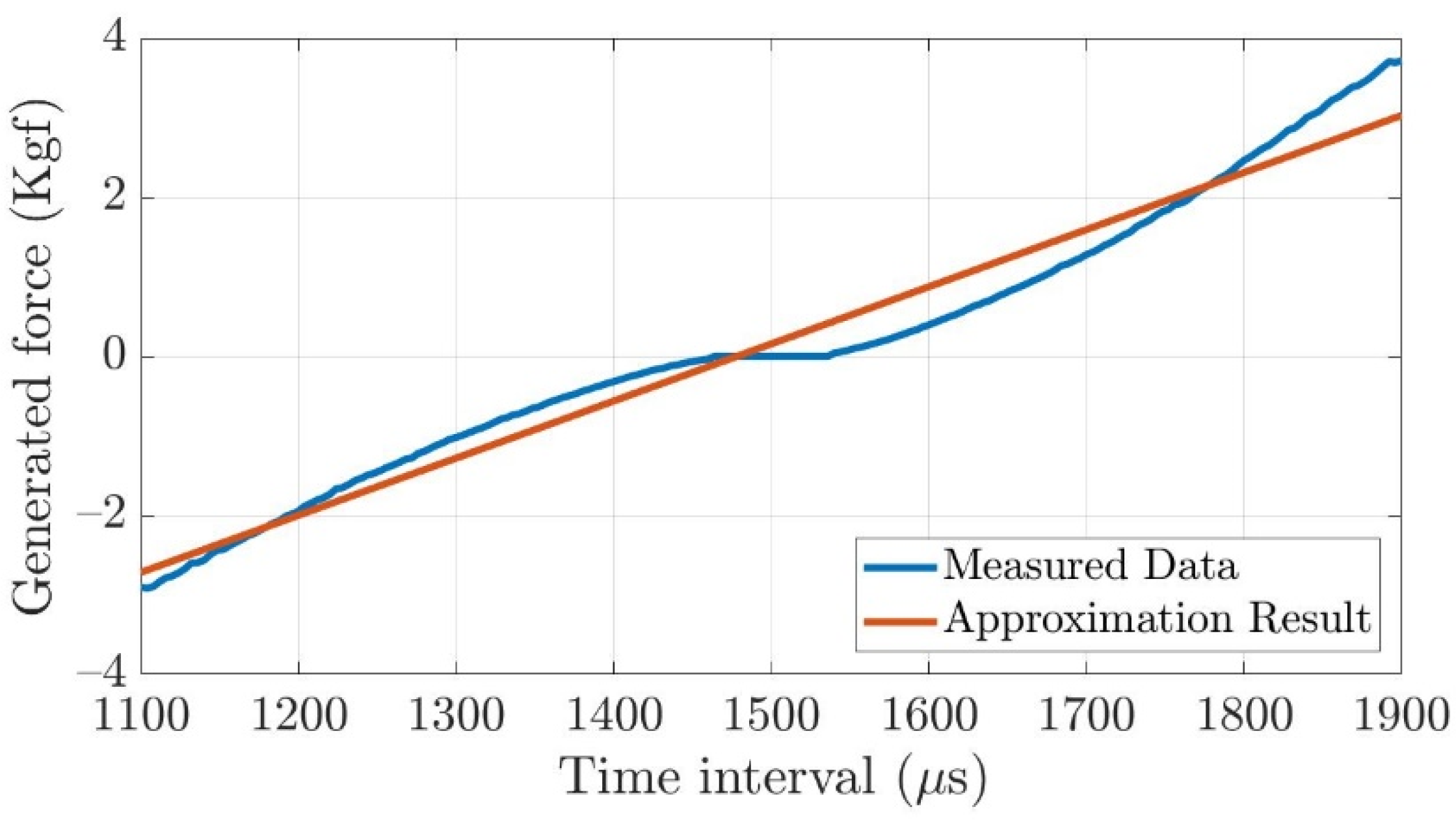
4.3.2. The Actuator Model of the Thruster
4.4. Control Allocation Verification for a Torpedo-Like Underwater Vehicle
- Step 1.
- Solve the control allocation of the fins and rudders.
- Step 2.
- Calculate the angle of fins and rudders.
- Step 3.
- Calculate the drag forces of the fins and rudders by using Equation (26).
- Step 4.
- Calculate the thruster force by the desired control law and compensation of drag forces.
- Step 5.
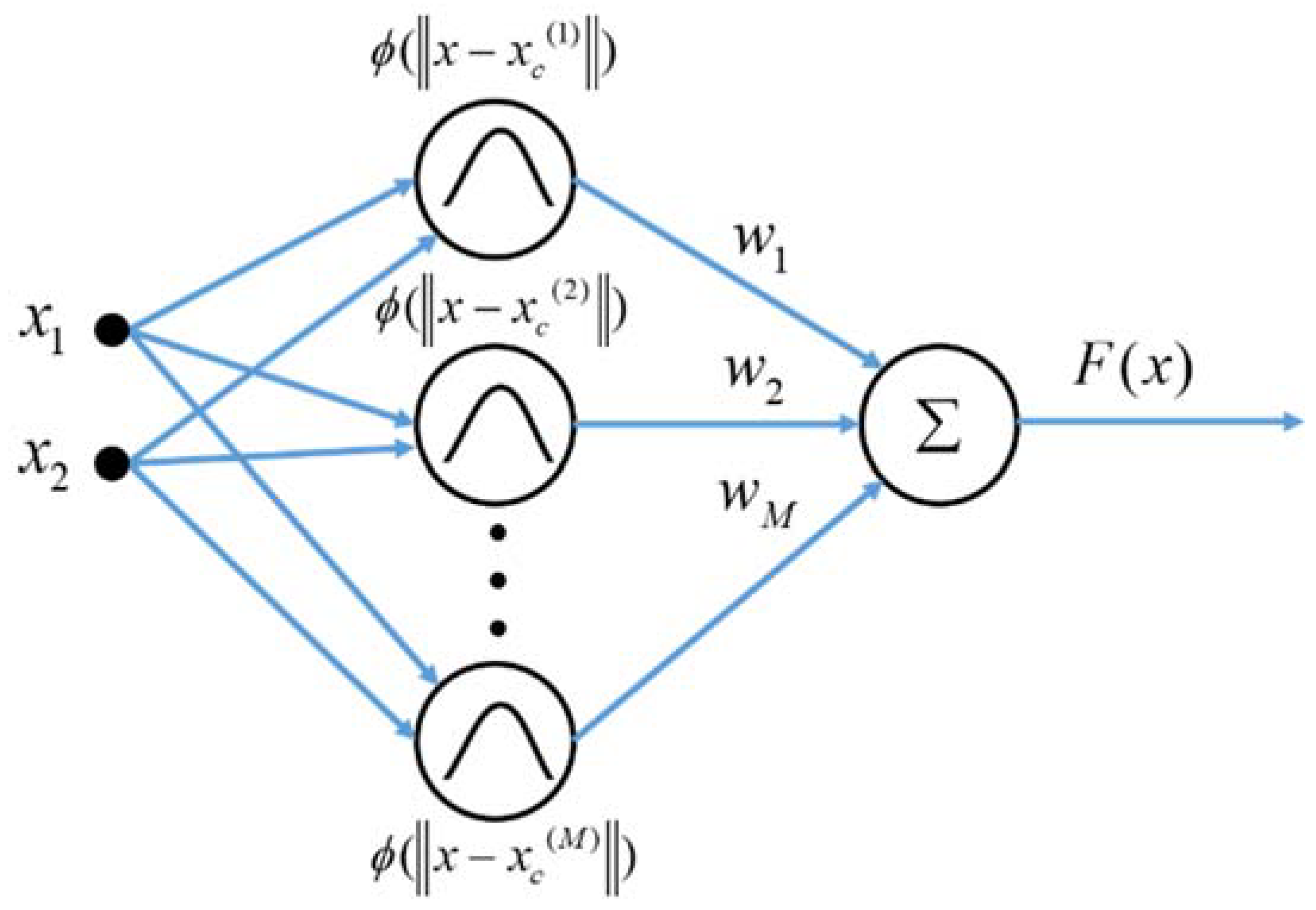
- Calculate the PWM signal of the thruster by using the radial basis function network.
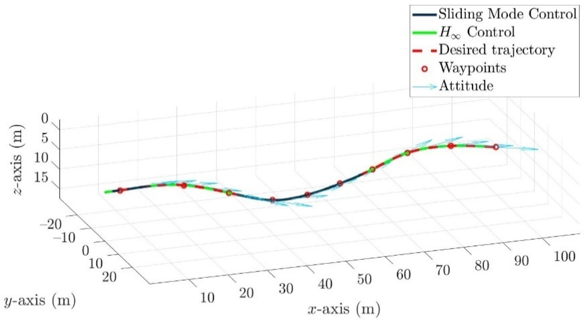
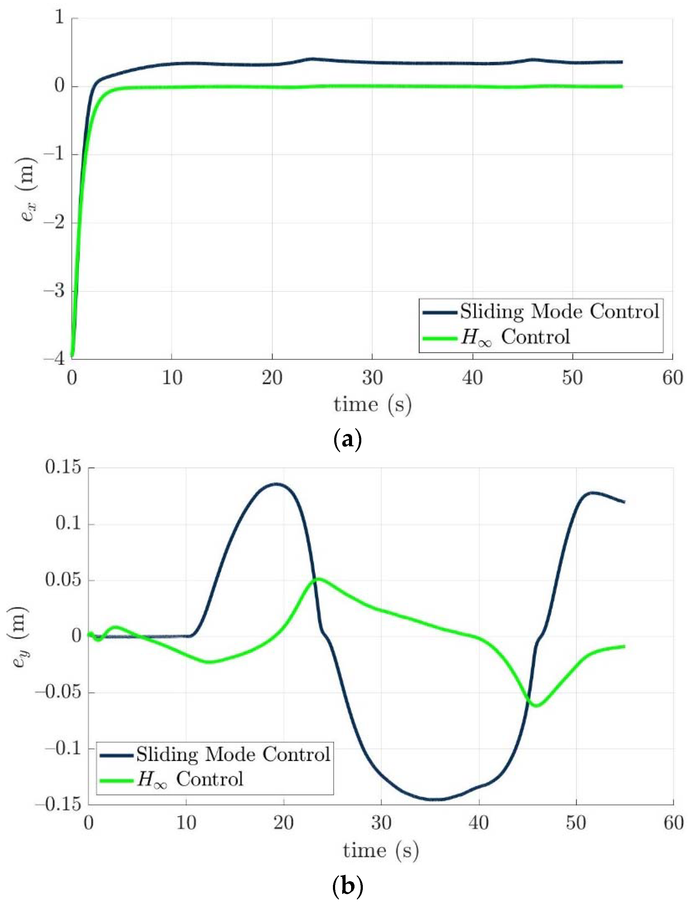
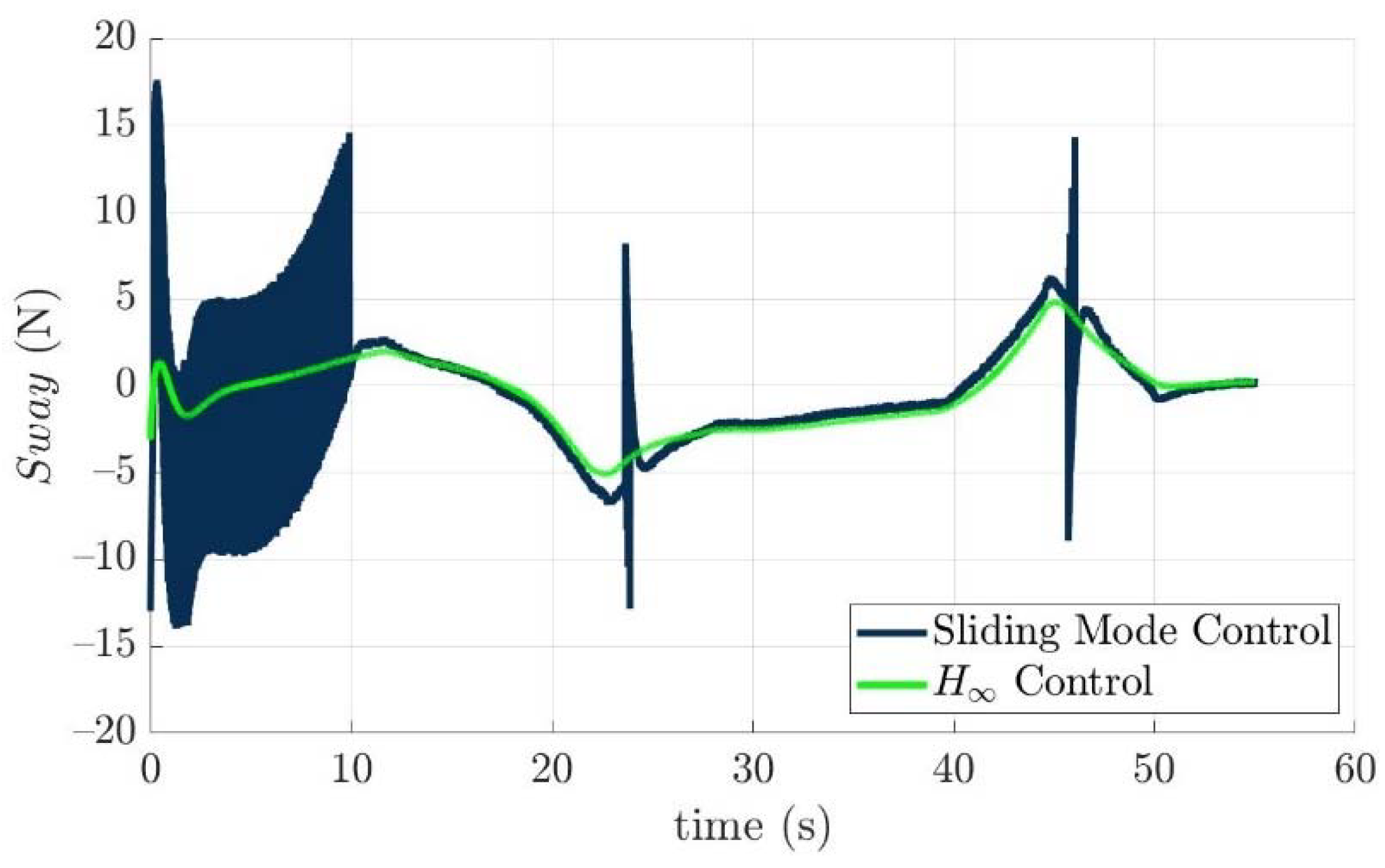
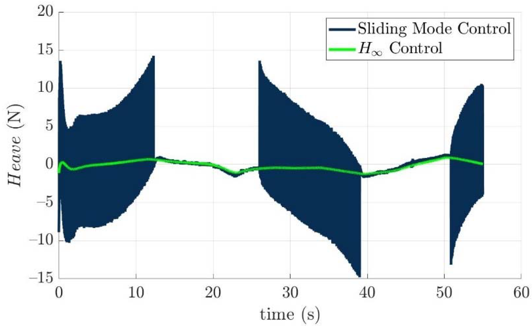
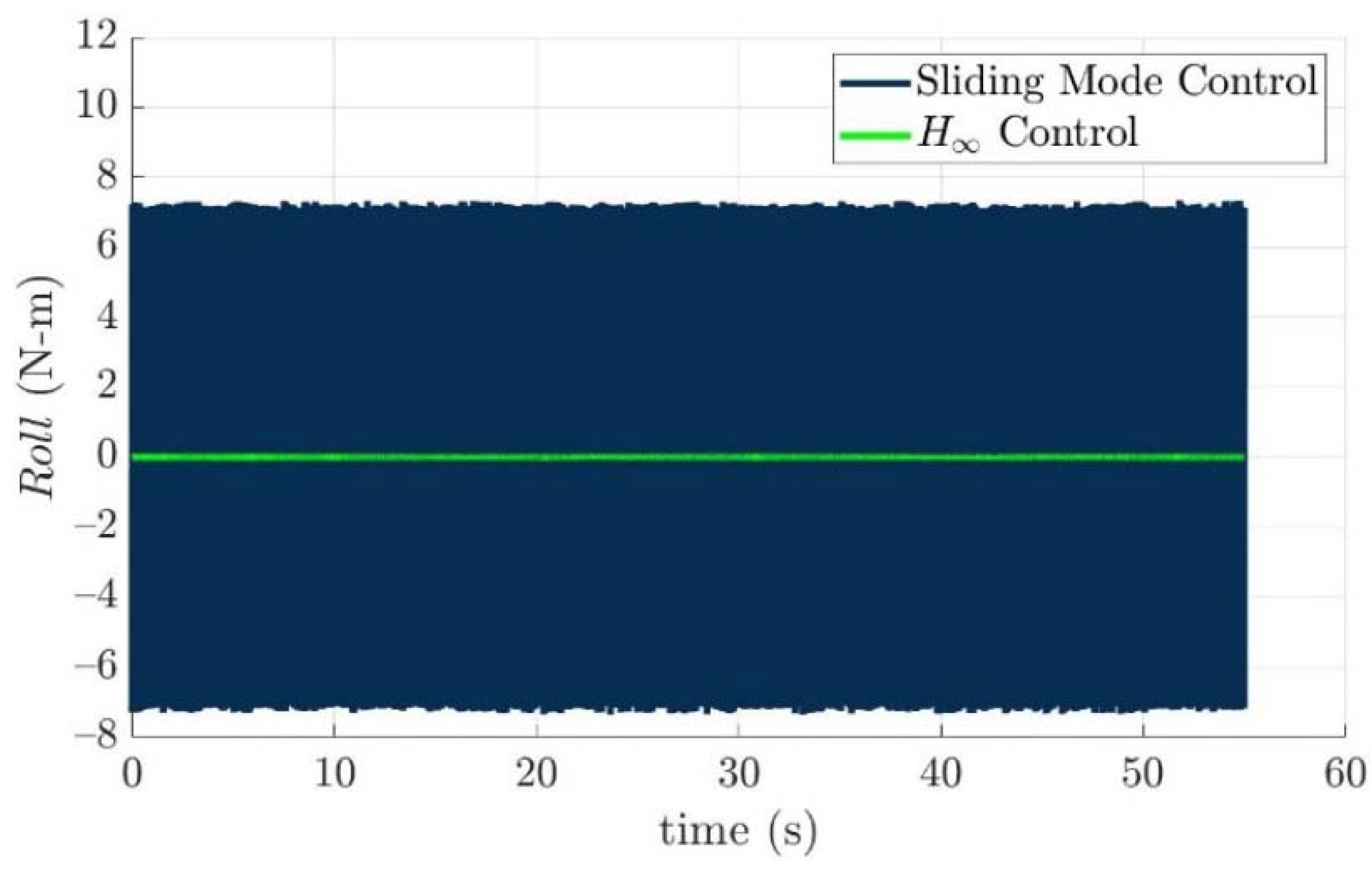
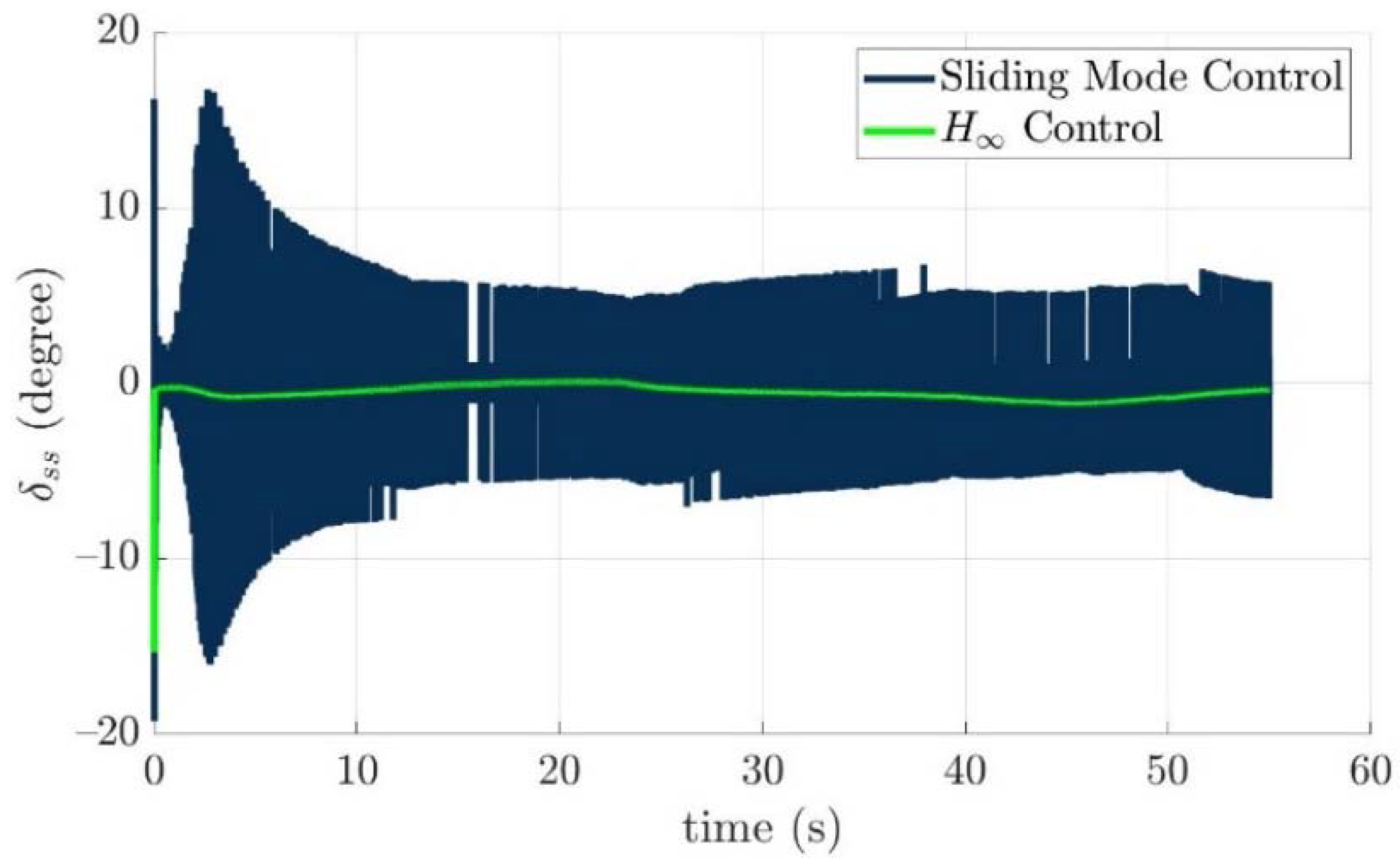
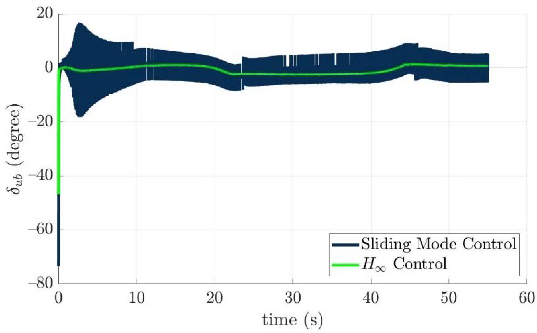
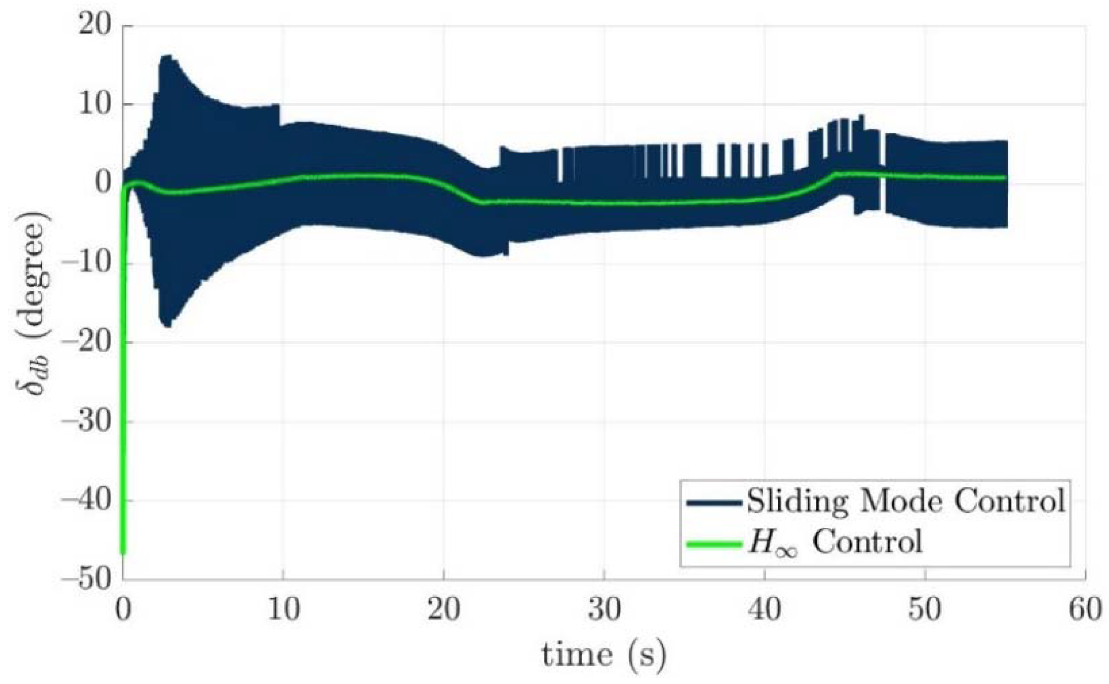
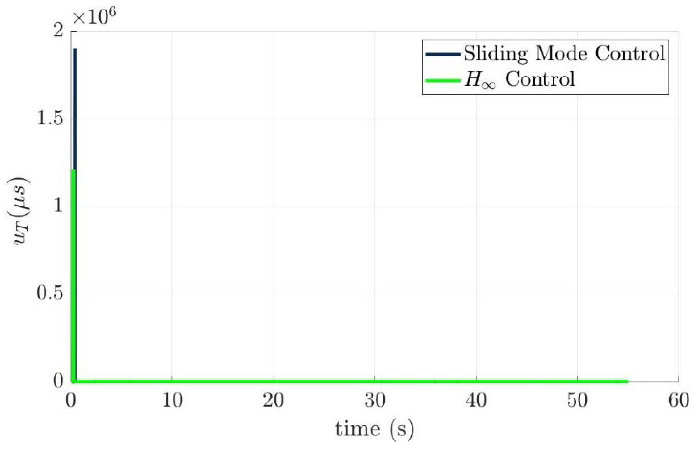
Scenario 1
5. Conclusions
Author Contributions
Funding
Institutional Review Board Statement
Informed Consent Statement
Data Availability Statement
Conflicts of Interest
Appendix A
Derivation of Radial Basis Function Network
References
- Fernandez, R.A.S.; Grande, D.; Martins, A.; Bascetta, L.; Dominguez, S.; Rossi, C. Modeling and Control of Underwater Mine Explorer Robot UX-1. IEEE Access 2019, 7, 39432–39447. [Google Scholar] [CrossRef]
- Hussain, N.A.A.; Ali, S.S.A.; Ovinis, M.; Arshad, M.R.; Al-Saggaf, U.M. Underactuated Coupled Nonlinear Adaptive Control Synthesis Using U-Model for Multivariable Unmanned Marine Robotics. IEEE Access 2019, 8, 1851–1865. [Google Scholar] [CrossRef]
- Valeriano, Y.; Fernandez, A.; Hernandez, L.; Prieto, P. Yaw Controller in Sliding Mode for Underwater Autonomous Vehicle. IEEE Lat. Am. Trans. 2016, 14, 1213–1220. [Google Scholar] [CrossRef]
- Gonzalez-Garcia, A.; Castaneda, H. Guidance and Control Based on Adaptive Sliding Mode Strategy for a USV Subject to Uncertainties. IEEE J. Ocean. Eng. 2021, 46, 1144–1154. [Google Scholar] [CrossRef]
- Chachada, M.; Vachhani, L.; Kartik, V. Empirical waypoint navigator for over actuated autonomous underwater vehicle using novel kinematic-dynamic controller pair and control allocation techniques. In Proceedings of the 2016 Indian Control Conference (ICC), Hyderabad, India, 4–6 January 2016; pp. 354–361. [Google Scholar] [CrossRef]
- Chin, C.S.; Lau, M.W.S.; Low, E.; Seet, G.G.L. A Cascaded Nonlinear Heading Control with Thrust Allocation: An Application on an Underactuated Remotely Operated Vehicle. In Proceedings of the 2006 IEEE Conference on Robotics, Automation and Mechatronics, Bangkok, Thailand, 1–3 June 2006; pp. 1–6. [Google Scholar] [CrossRef]
- Ji, S.; Jang, J.; Jeong, J.; Kim, Y. The H∞ controller design including control allocation for marine vessel. In Proceedings of the 2012 12th International Conference on Control, Automation and Systems, Jeju Island, Korea, 17–21 October 2012; pp. 1905–1907. [Google Scholar]
- Shen, C.; Shi, Y.; Buckham, B. Lyapunov-based model predictive control for dynamic positioning of autonomous underwater vehicles. In Proceedings of the 2017 IEEE International Conference on Unmanned Systems (ICUS), Beijing, China, 27–29 October 2017; pp. 588–593. [Google Scholar] [CrossRef]
- Yu, C.; Xiang, X.; Wilson, P.; Zhang, Q. Guidance-Error-Based Robust Fuzzy Adaptive Control for Bottom Following of a Flight-Style AUV with Saturated Actuator Dynamics. IEEE Trans. Cybern. 2019, 50, 1887–1899. [Google Scholar] [CrossRef] [PubMed]
- Johansen, T.A.; Fossen, T.I. Control allocation—A survey. Automatica 2013, 49, 1087–1103. [Google Scholar] [CrossRef] [Green Version]
- Oppenheimer, M.W.; Doman, D.B.; Bolender, M.A. Control allocation for over-actuated systems. In Proceedings of the 2006 14th Mediterranean Conference on Control and Automation, Ancona, Italy, 28–30 June 2006; pp. 1–6. [Google Scholar] [CrossRef]
- Fossen, T.I.; Johansen, T.A. A survey of control allocation methods for ships and underwater vehicles. In Proceedings of the 2006 14th Mediterranean Conference on Control and Automation, Ancona, Italy, 28–30 June 2006; pp. 1–6. [Google Scholar] [CrossRef]
- Fossen, T.I.; Johansen, T.A. A Survey of Control Allocation Methods for Ships and Underwater Vehicles. Underw. Veh. 2009, 110–128. [Google Scholar] [CrossRef] [Green Version]
- Khan, H.Z.I.; Rajput, J.; Ahmed, S.; Sarmad, M.; Sharjil, M. Robust control of overactuated autonomous underwater vehicle. In Proceedings of the 2018 15th International Bhurban Conference on Applied Sciences and Technology (IBCAST), Islamabad, Pakistan, 9–13 January 2018; pp. 269–275. [Google Scholar] [CrossRef]
- Soylu, S.; Buckham, B.J.; Podhorodeski, R.P. Robust Control of Underwater Vehicles with Fault-Tolerant Infinity-Norm Thruster Force Allocation. Oceans 2007, 1–10. [Google Scholar] [CrossRef]
- Yinghao, Z.; Jiangfeng, Z.; Yueming, L.; Yushan, S.; Lei, W.; Shuling, H. Research on reconstructive fault-tolerant control of an X-rudder AUV. In Proceedings of the OCEANS 2016 MTS/IEEE Monterey, Monterey, CA, USA, 19–23 September 2016; pp. 1–5. [Google Scholar] [CrossRef]
- Tolstonogov, A.; Kostenko, V. AUV thrust allocation with variable constraints. Adv. Syst. Sci. Appl. 2017, 17, 1–8. [Google Scholar]
- Yi-Sheng, Y. Design of Adaptive Fuzzy Guidance Law for Autonomous Underwater Vehicles: Mixed H2/H∞ Approach; National Cheng Kung University: Tainan, Taiwan, 2020. [Google Scholar]
- Ke, S.; Jinchuan, Z.; Hai, W.; Xueqian, W.; Renquan, L.; Zhihong, M. Tracking Control of a Linear Motor Positioner Based on Barrier Function Adaptive Sliding Mode. IEEE Trans. Ind. Inform. 2021, 17, 7479–7488. [Google Scholar] [CrossRef]


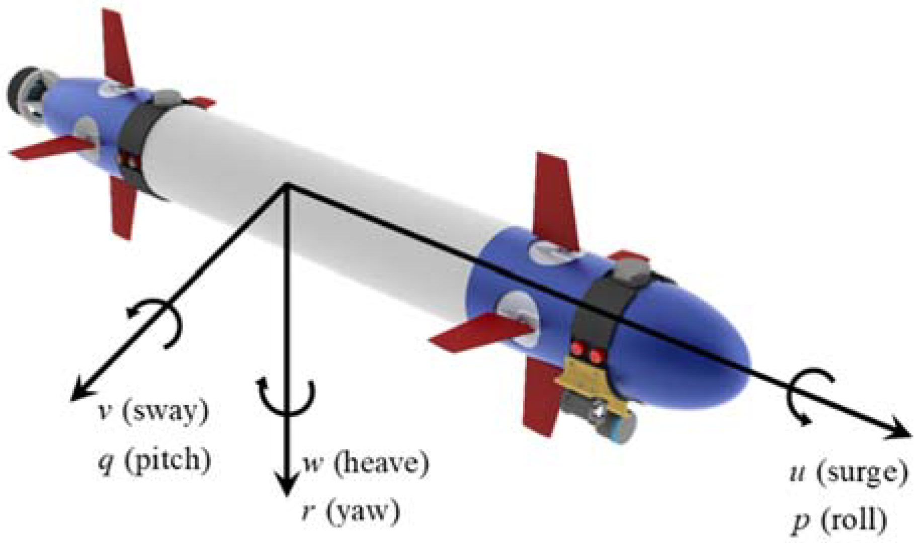
| DOF | Linear and Angular Velocities | Positions and Euler Angles | Forces and Moments | |
|---|---|---|---|---|
| 1 | Motions in the x-direction (surge) | u | x | X |
| 2 | Motions in the y-direction (sway) | υ | y | Y |
| 3 | Motions in the z-direction (heave) | w | z | Z |
| 4 | Rotations about the x-axis (roll) | p | ϕ | K |
| 5 | Rotations about the y-axis (pitch) | q | θ | M |
| 6 | Rotations about the z-axis (yaw) | r | ψ | N |
| Parameter | Value |
|---|---|
| Total length L | 1.54 m |
| Nose length a | 0.15 m |
| Midbody length b | 1.14 m |
| Tail length c | 0.25 m |
| Hull diameter d | 0.16 m |
| Mass m | 14.56 kg |
| Buoyancy B | 27.13 kg |
| Moment of inertia Ix | 0.072 kg·m2 |
| Moment of inertia Iy | 12.02 kg·m2 |
| Moment of inertia Iz | 12.02 kg·m2 |
| Actuator | Position (cm) | Generated Force | Control Command |
|---|---|---|---|
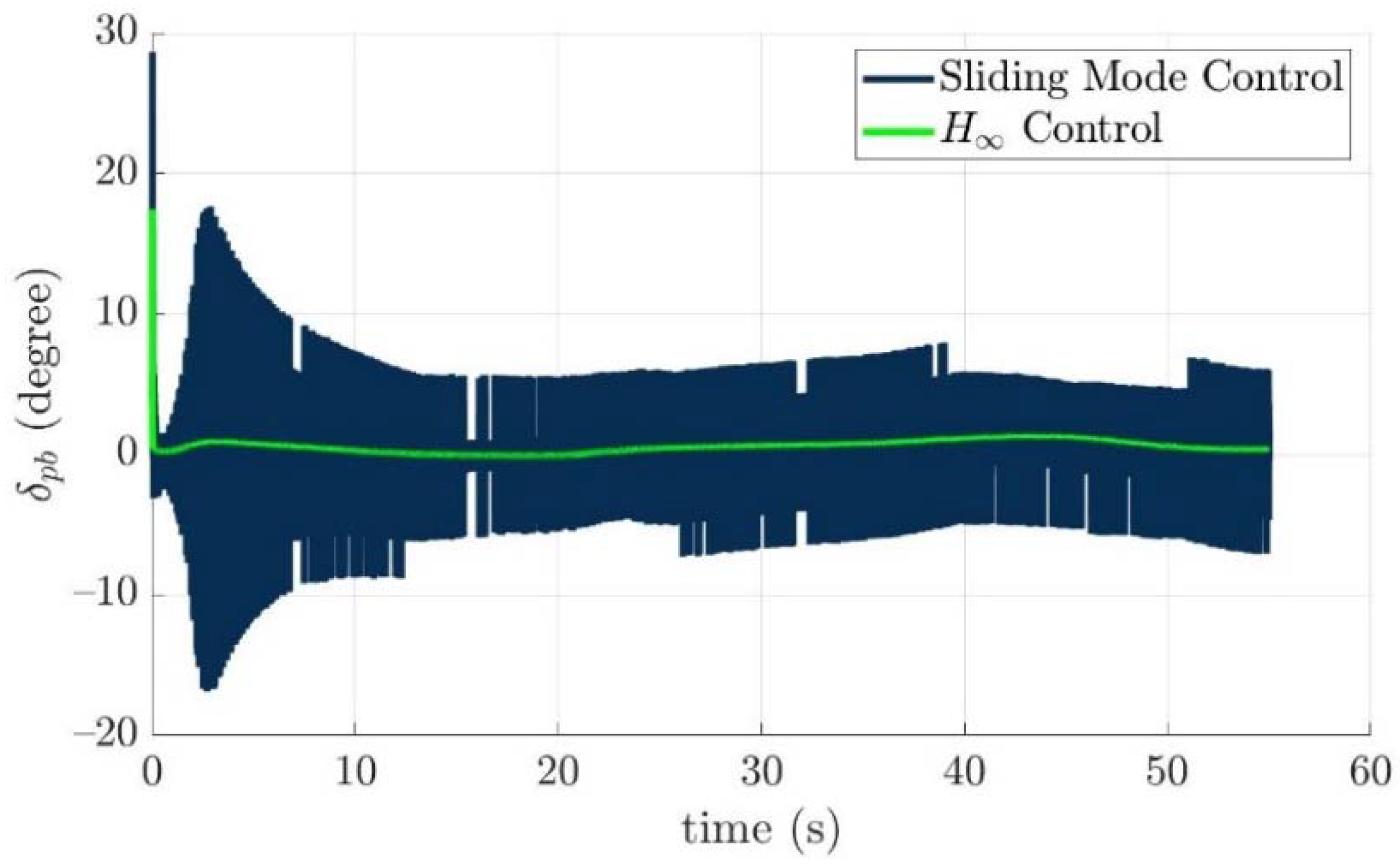
| Port bow fin | (39, −16, 0) | [0 0 −Fpb] | δpb (degree) |
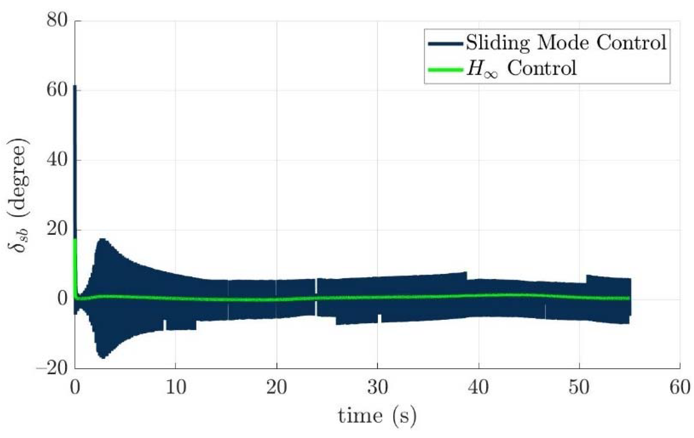
| Starboard bow fin | (39, 16, 0) | [0 0 −Fsb] | δsb (degree) |
| Upward bow rudder | (39, 0, −16) | [0 Fub 0] | δub (degree) |
| Downward bow rudder | (39, 0, 16) | [0 Fdb 0] | δdb (degree) |
| Port stern fin | (−57, −16, 0) | [0 0 −Fps] | δps (degree) |
| Starboard stern fin | (−57, 16, 0) | [0 0 −Fss] | δss (degree) |
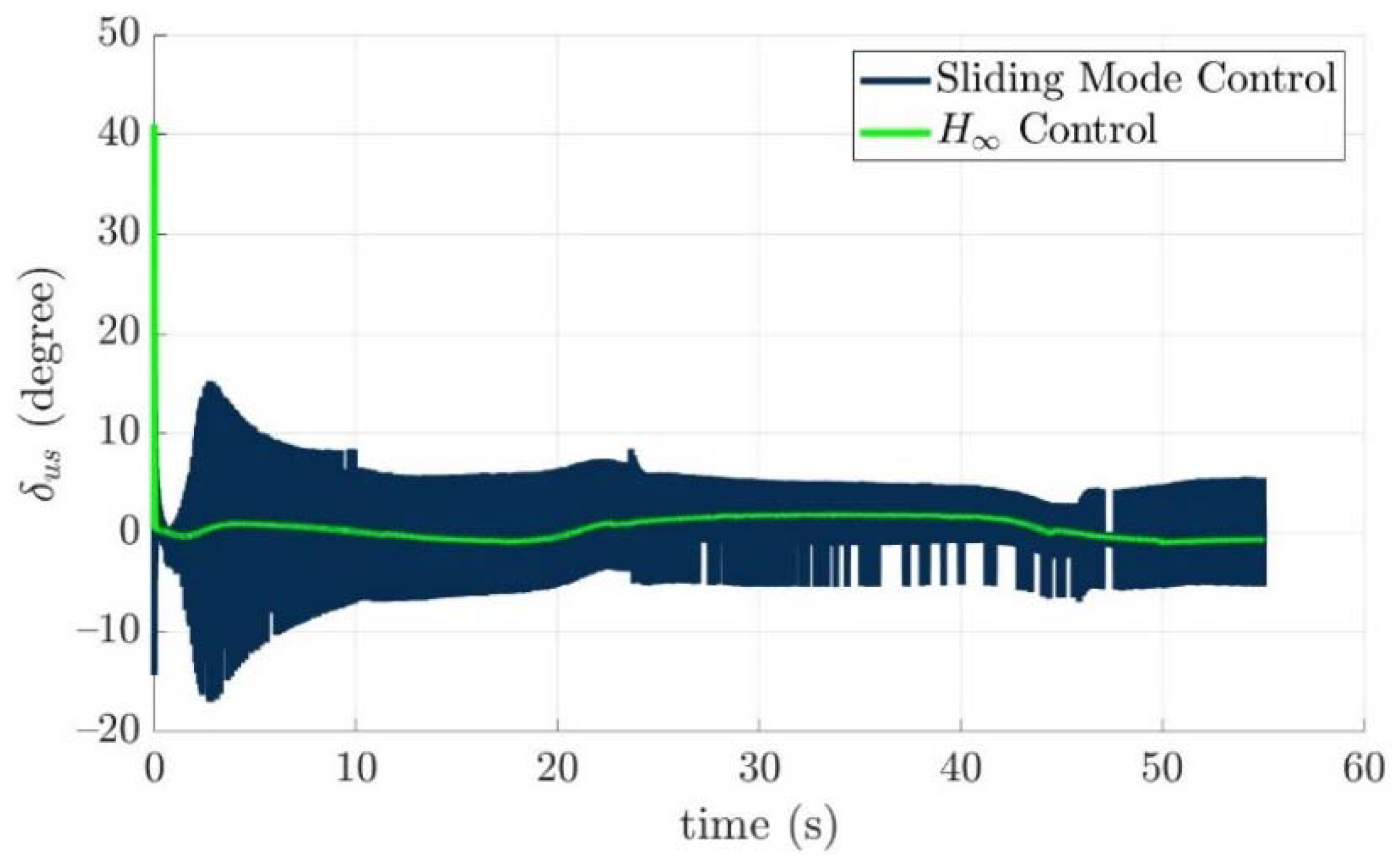
| Upward stern rudder | (−57, 0, −16) | [0 Fus 0] | δus (degree) |
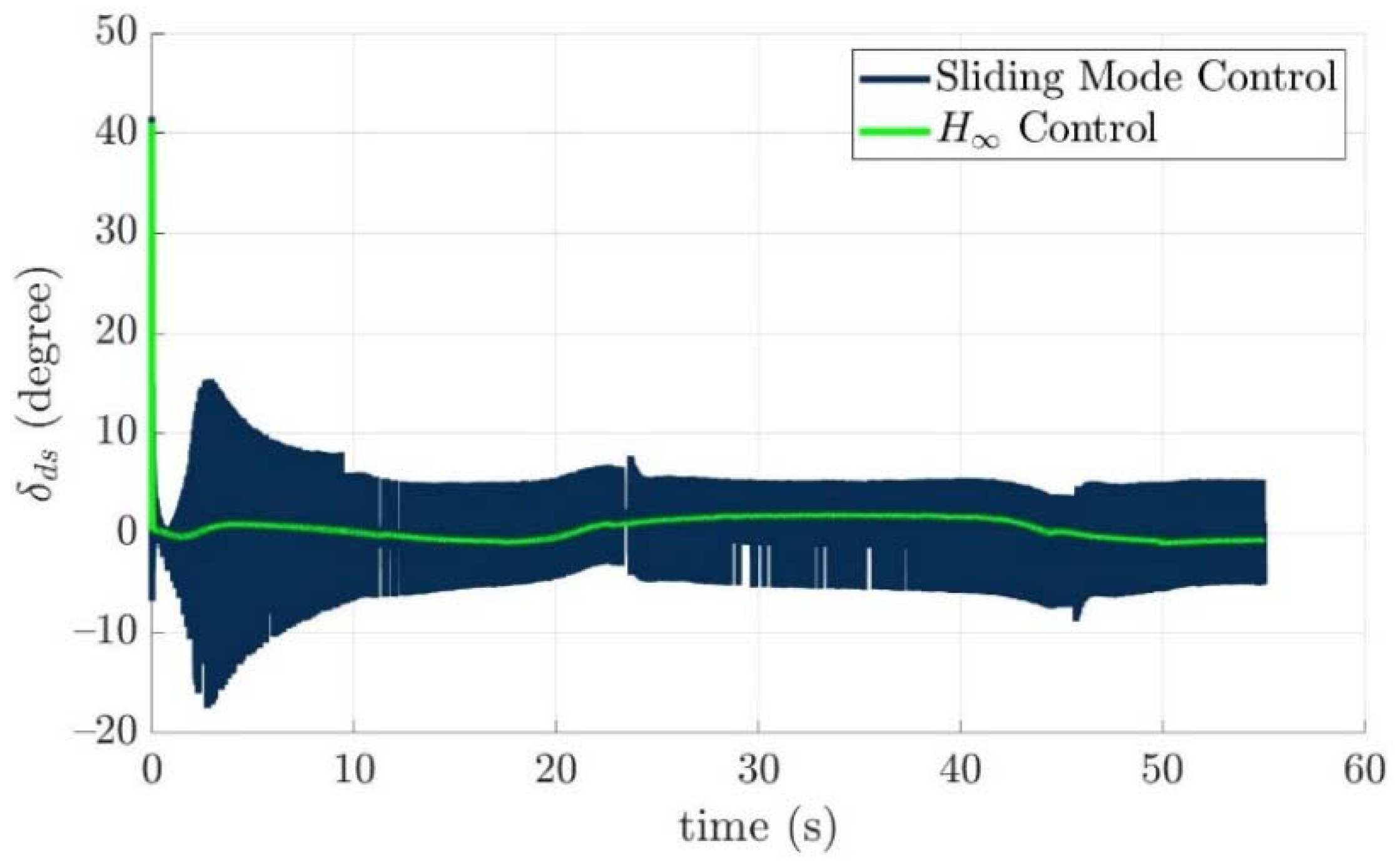
| Downward stern rudder | (−57, 0, 16) | [0 Fds 0] | δds (degree) |
| Thruster | (−80, 0, 0) | [FT 0 0] | uT (PWM) |
| No. | Waypoints (x, y, z) (m) | No. | Waypoints (x, y, z) (m) |
|---|---|---|---|
| 1 | (4, 0, 5) | 6 | (60, 0, 9.8) |
| 2 | (20, 0.75, 5.3) | 7 | (70, −5, 9) |
| 3 | (30, 5, 7) | 8 | (80, −8, 7) |
| 4 | (40, 8, 9) | 9 | (90, −5, 5.4) |
| 5 | (50, 5, 9.8) | 10 | (100, −0.85, 5.5) |
| Parameter | Value |
|---|---|
| λ1 | 4 |
| λ2 | 4 |
| Γ | |
| Z |
| Parameter | Value |
|---|---|
| λf1 | 4 |
| λf2 | 4 |
| ksc | 7 |
| ks | 4 |
Publisher’s Note: MDPI stays neutral with regard to jurisdictional claims in published maps and institutional affiliations. |
© 2022 by the authors. Licensee MDPI, Basel, Switzerland. This article is an open access article distributed under the terms and conditions of the Creative Commons Attribution (CC BY) license (https://creativecommons.org/licenses/by/4.0/).
Share and Cite
Chen, Y.-Y.; Lee, C.-Y.; Huang, Y.-X.; Yu, T.-T. Control Allocation Design for Torpedo-Like Underwater Vehicles with Multiple Actuators. Actuators 2022, 11, 104. https://doi.org/10.3390/act11040104
Chen Y-Y, Lee C-Y, Huang Y-X, Yu T-T. Control Allocation Design for Torpedo-Like Underwater Vehicles with Multiple Actuators. Actuators. 2022; 11(4):104. https://doi.org/10.3390/act11040104
Chicago/Turabian StyleChen, Yung-Yue, Chun-Yen Lee, Ya-Xuan Huang, and Tsung-Tso Yu. 2022. "Control Allocation Design for Torpedo-Like Underwater Vehicles with Multiple Actuators" Actuators 11, no. 4: 104. https://doi.org/10.3390/act11040104