Fractional Order PID Control Based on Ball Screw Energy Regenerative Active Suspension

Abstract

A ball screw type energy regenerative active suspension under fractional order PID control is proposed and studied in order to improve the vibration damping performance of the suspension. A mathematical model of the energy regenerative actuator is established, the energy recovery power at different frequencies is measured through experiments, and then the electromagnetic torque constant, representing the proportional relationship between the output torque and current of the motor, is calculated according to the experimental results. A mathematical model of the control circuit is established and the feasibility and the superiority of the fractional order PID control are verified by simulation and experiments. To achieve a better damping effect, the fractional order PID controller of the whole vehicle suspension system is parameterized using the Beetle Antenna Search (BAS) algorithm. The results showed that the mean energy recovery power of the actuator was about 3.5091 W at a vibration frequency of 11/6 Hz, and the electromagnetic torque constant of the motor was about 0.2885. The actuator control circuit was feasible, and the root mean square value of current deviation under fractional order PID control was 1.1158 mA, which was optimized by 9.40%, compared to the PID control. The BAS algorithm effectively realized the parameter tuning of the controller, and both the tuned PID and fractional order PID controllers, achieved optimization of suspension damping performance. The optimal value of the damping performance objective function under fractional order PID control was 0.3270, which was optimized by 62.93%, compared to the PID control. In addition, all suspension performance indices under fractional order PID control were optimized to a certain extent, compared with the PID control.

1. Introduction

With the continuous development of the automotive industry, the requirements for smoothness and handling stability of vehicles are increasing, and research on semi-active and active suspensions has become a hot topic [1,2,3,4]. In order to follow the international trend of sustainable energy use, energy recovery has also become an important direction in suspension research. Therefore, the study of energy regenerative active suspensions [5,6], which can achieve active control and energy recovery at the same time, has become an important breakthrough point.

The central issue in the study of energy regenerative suspensions is the design of the energy regenerative actuators. Amini [7] designed an energy regenerative rotary damper with a rack and pinion mechanism to convert the linear motion of the suspension deformation into a rotational motion of the drive motor to generate energy, while Zhang [8] proposed an electro-hydraulic damper for energy harvesting. Zhu [9] modelled and studied a linear electromagnetic device for vibration damping and energy harvesting. The above energy regenerative actuator designs have been effective in improving vehicle comfort and achieving energy recovery. In this paper, a ball screw type energy regenerative actuator [10] was used to build the energy regenerative suspension. When working in energy regenerative mode, the actuator converts the linear motion of the suspension vibration into rotary motion through the ball screw mechanism, and the motor shaft rotates to generate electrical energy, thus, charging the vehicle’s power supply or powering other power-consuming components, such as the suspension controller and body accelerometer. When working in active control mode, the controller takes active control of the actuator and outputs active control force, thus, achieving vibration reduction of the vehicle.

The core problem of studying active suspension control is the study of its control algorithm. Among various active control algorithms, the PID controller is widely used because of its simple algorithm, stable control ability, good robustness and other advantages. Narwade [11] studied the modelling and simulation of an automotive semi-active suspension system based on the PID controller, and conducted a simulation study for the application of the PID controller on automotive suspension in a more systematic way. Nagarkar [12] used PID and fuzzy control, based on a genetic algorithm, for an active non-linear 1/4 automotive suspension system to achieve multi-objective optimization of the suspension system. Although the above studies have achieved the optimization of suspension damping performance under passive suspension or classical PID control, it is still difficult to fundamentally solve the limitation of the PID controller control precision. In the PID control process [13], the stronger the proportional link P is, the faster the system response will be, but if it is too strong this will lead to system oscillation and destroy the stability of the system. The stronger the integral link I is, the faster the system static error can be eliminated, but if it is too strong this will produce the phenomenon of integral saturation, causing the system overshoot to increase. The role of differential link D is to stop the change of deviation, and it is controlled according to the trend of deviation, which can reduce the amount of overshoot, overcome oscillation and make the system more stable, but the role of the differential is sensitive to the noise of the input signal, so, for those systems with large noise, the strength of the differential link should be carefully chosen. This paper is aimed at the actuator control circuit and the whole vehicle suspension system under fractional order PID control. The fractional order PID controller [14] adds two control parameters $\lambda$ and $\mu$ to the PID controller, where λ refers to the fractional order of the integral link I in fractional order PID control, and μ refers to the fractional order of the differential link D in fractional order PID control. This allows the controller to have a larger range of parameters and higher control accuracy, so that the strength of the proportional, integral and differential links can be determined more precisely; thus, obtaining better circuit control and suspension damping performance.

In summary, among the existing types of suspensions, passive suspension is the most basic form, mainly consisting of dampers and elastic elements. Passive suspension is a traditional mechanical structure, which is simple in structure, reliable in performance, low in cost and does not require additional energy, and, thus, is widely used, but the damping and stiffness of passive suspension are unchangeable, so in the actual process of use, in the face of complex road conditions, it is difficult to achieve the optimal damping effect. In the process of damping, the energy generated by the suspension vibration is eventually dissipated in the form of heat, while the energy recovery type passive suspension [15] recovers this part of vibration energy by adding an energy regenerative actuator to reduce the waste of energy. However, since it does not have an active control process, there is still the problem that the stiffness and damping cannot be changed. Therefore, this paper investigated the energy regenerative active suspension, and through active control of the energy regenerative actuator, the output of the active control force of the suspension system was achieved, while ensuring energy recovery, so that the damping capacity of the suspension system could be optimized. This paper designed an energy regenerative active suspension composed of a ball screw type energy regenerative actuator, established a mathematical model of the energy regenerative actuator, calculated the electromagnetic torque constant of the energy regenerative actuator, through relevant formulae and energy regenerative tests and studied the fractional order PID control circuit through simulation and test of the control circuit. The dynamics model of the whole vehicle suspension system was established, and the whole vehicle suspension system was actively controlled by the PID and fractional order PID controller rectified by the Beetle Antenna Search algorithm. The Beetle Antenna Search algorithm was proposed by Jiang X and Li S [16] in 2017, with strong competitiveness, compared with the traditional parameter rectification algorithm [17], and compared with the Particle Swarm (PSO) algorithm. When caught in local extremes, the jump out capability of the Beetle Antenna Search algorithm is stronger and its convergence is faster than the Particle Swarm algorithm (PSO). Genetic algorithms (GAs) sometimes require binary coding and are computationally intensive, while BAS algorithms do not and are computationally much faster than GAs. Compared with the Bat algorithm (BA) and Artificial Bee Colony (ABC) algorithm, it is more efficient and has very low complexity. Besides, the BAS algorithm is more efficient, as it is lower than most swarm intelligence algorithms, in terms of time and space complexity. The simulation verified the parameter seeking effect of the algorithm and fully analyzed the optimization of each performance index based on the simulation results.

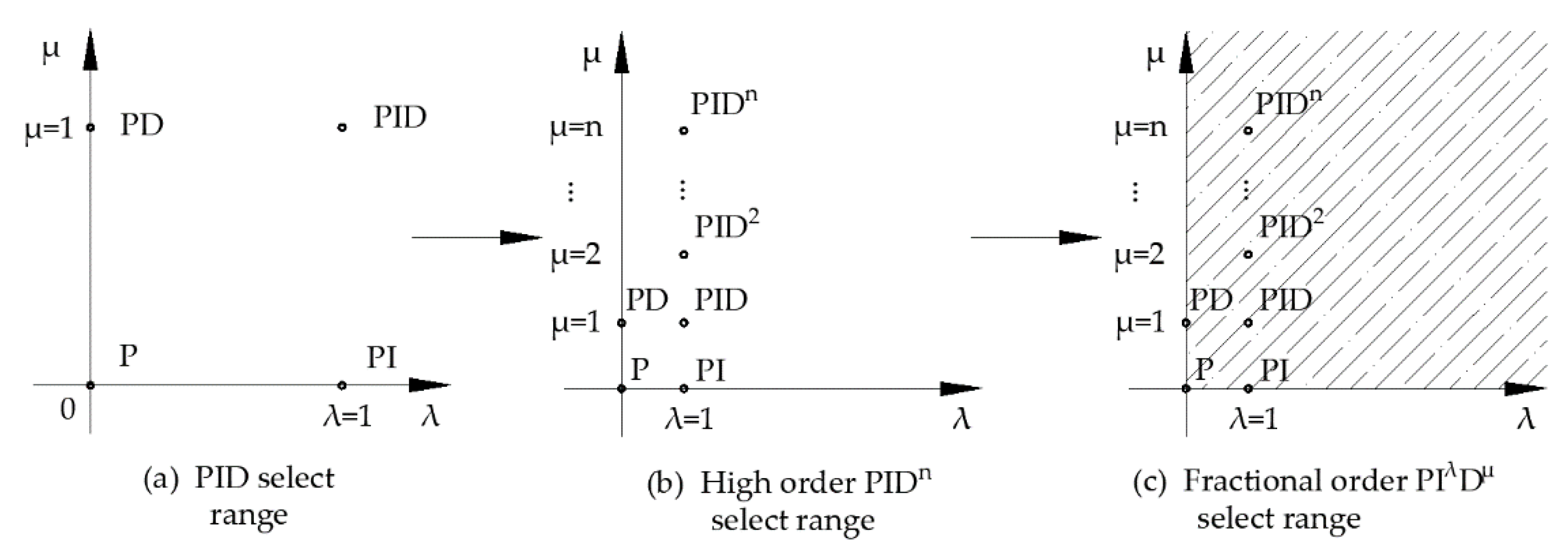
2. Advanced Fractional Order PID Controller

As shown in Figure 1 below, since the values of n in the figure are arbitrary integers and the values of λ and μ are arbitrary real numbers, the conventional integer order PID controller can only vary at a few fixed points in the figure in the plane constructed by P-I-D, as shown in Figure 1a. In contrast, the PID controller with higher order integral links and higher order differential links [18], which is extended on this basis, increases the number of selectable points, as shown in Figure 1b. The fractional order PID control controller can select any point on the plane, and the range of parameter rectification is changed from ‘point’ to ‘surface’, as shown in Figure 1c. This makes the structure of the fractional order PID controller more flexible and more adaptable to the dynamic characteristics of complex control systems, so it is very important in research of fractional order PID control. It should be noted that the above is the setting range of the fractional order PID parameters under ideal conditions. In actual conditions, the implementation of fractional operators, by higher order filters, does not strictly ensure continuous coverage of the plane of selectable fractional parameters, just an approximation.

3. Principles and Modelling

3.1. Working Principle of Energy Regenerative Active Suspension

The structure of the 1/4 energy regenerative active suspension is shown in Figure 2, which mainly consists of a spring, a damper, a ball screw type energy regenerative actuator, a controller, an energy regenerative circuit, a battery and a body acceleration sensor, of which the ball screw type energy regenerative actuator consists of an energy regenerative motor and a ball screw mechanism. In the energy regenerative mode, the suspension vibration causes the ball screw mechanism to move, and the ball screw mechanism drives the energy regenerative motor to rotate, generating electrical energy to charge the battery through the energy regenerative circuit, which, in turn, uses the energy for the suspension control circuit or supplies it to other energy-consuming parts of the vehicle, thus realizing energy recovery and reuse. In active control mode, the body accelerometer transmits the collected signals to the controller, which then transmits the processed signals to the control circuit, which drives the energy regenerative actuator to output active control force, thus realizing active control of the suspension system and improving driving smoothness.

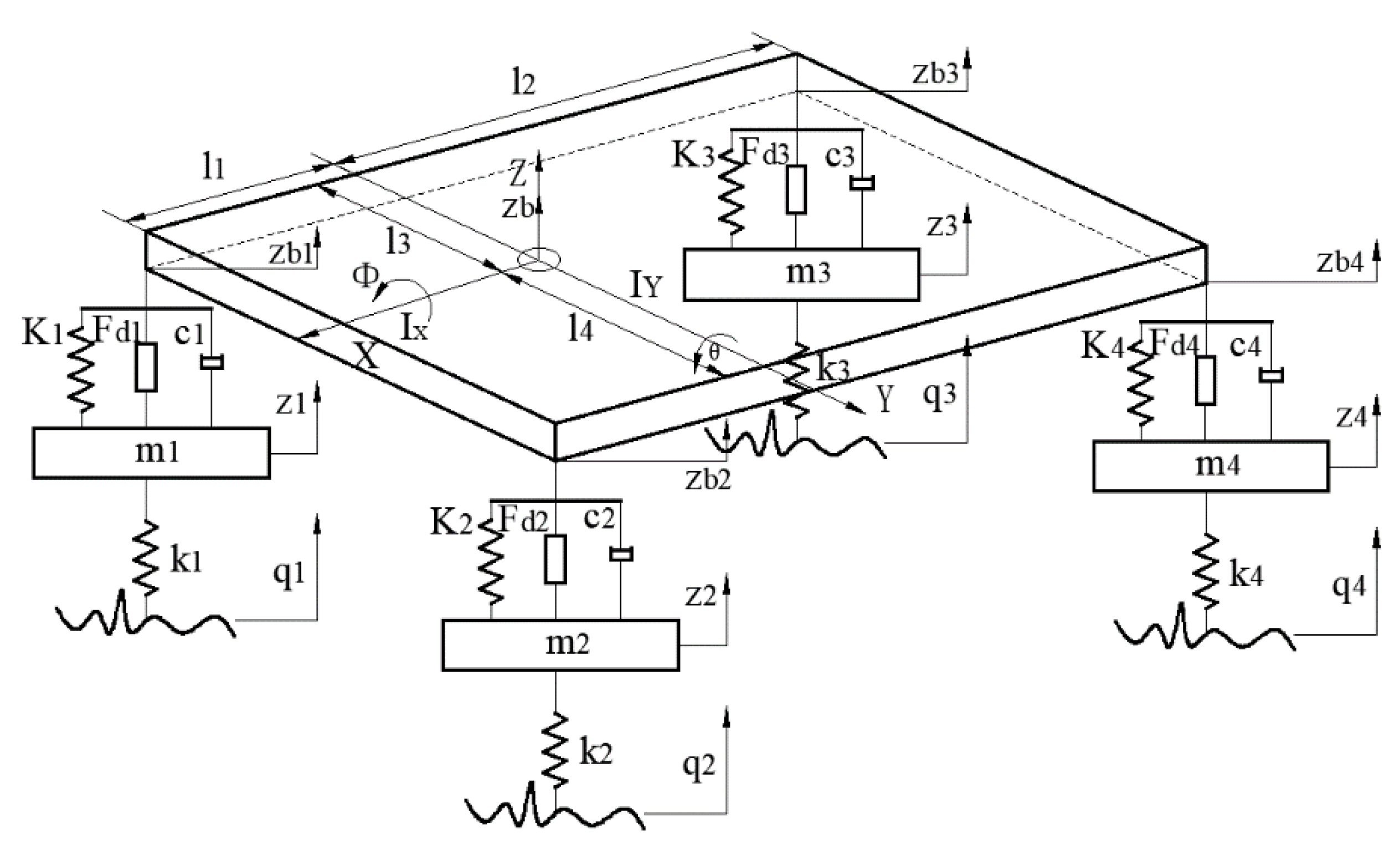
3.2. Dynamics Model of the Whole Vehicle Energy Regenerative Active Suspension System

In order to achieve a comprehensive analysis of the damping performance of the energy regenerative active suspension, a 7-DOF suspension system dynamics model for the whole vehicle was developed with reference to the 1/4 energy regenerative active suspension structure, as shown in Figure 3.

In the Figure 3, $l_1$, $l_2$ are the lengths from the body centroid to the front axis and rear axis of the body, respectively, while $l_3$, $l_4$ are the lengths from the body centroid to the center lines of the left and right tires. Values $I_X,I_Y$ are the rotational inertia of the body around axis X and axis Y, respectively. The body roll angular shift for the X axis is $\varphi$, and $\theta$ is the body pitching angular shift for the Y axis. Values $q_1~q_4$ are the road excitation input to each wheel, $k_1~k_4$ are the equivalent stiffness of each tire, $z_1~z_4$ are the vertical vibration displacement of the mass $m_1~m_4$ under each spring, $K_1~K_4$ are the stiffness of elastic components in each suspension system.${\mathrm{Values}c}_1~c_4$ are equivalent damping, due to electromagnetic torque of energy regenerative shock absorber, $F_{d1}~F_{d4}$ are the active control forces of suspension system and $z_{b1}~z_{b4}$ are the auxiliary displacements in the derivation of suspension dynamics mathematical model. When the pitching angular and roll angular are small, the relation between the auxiliary displacement and the displacement of body center of mass $z_b$ is shown in Equation (1) below:

$$\{\begin{array}{l}{z}_{b1}=z_b-l_3\varphi -l_1\theta ,z_{b2}=z_b+l_4\varphi -l_1\theta \\ z_{b3}=z_b-l_3\varphi +l_2\theta ,z_{b4}=z_b+l_4\varphi +l_2\theta \end{array}$$

(1)

The differential equations of motion for the center of mass of the suspension system, the differential equation of roll motion, the differential equation of pitching motion and the four differential equations of motion for the under-spring mass are obtained as shown in Equations (2), (3), (4) and (5), respectively.

$$\begin{array}{l}{\mathrm{m}}_b{\ddot{z}}_b+K_1(z_b-l_3\varphi -l_1\theta -z_1)+K_2(z_b+l_4\varphi -l_1\theta -z_2)+K_3(z_b-l_3\varphi +l_2\theta -z_3)\\ +K_4(z_b+l_4\varphi +l_2\theta -z_4)+c_1({\dot{z}}_b-l_3\dot{\varphi }-l_1\dot{\theta }-{\dot{z}}_1)+c_2({\dot{z}}_b+l_4\dot{\varphi }-l_1\dot{\theta }-{\dot{z}}_2)+\\ c_3({\dot{z}}_b-l_3\dot{\varphi }+l_2\dot{\theta }-{\dot{z}}_3)+c_4({\dot{z}}_b+l_4\dot{\varphi }+l_2\dot{\theta }-{\dot{z}}_4)-F_{d1}-F_{d2}-F_{d3}-F_{d4}=0\end{array}$$

(2)

$$\begin{array}{l}{I}_X\ddot{\varphi }-l_3[K_1(z_b-l_3\varphi -l_1\theta -z_1)+c_1({\dot{z}}_b-l_3\dot{\varphi }-l_1\dot{\theta }-{\dot{z}}_1)-F_{d1}+K_3(z_b-l_3\varphi +l_2\theta -z_3)\\ +c_3({\dot{z}}_b-l_3\dot{\varphi }+l_2\dot{\theta }-{\dot{z}}_3)-F_{d3}]+l_4[K_2(z_b+l_4\varphi -l_1\theta -z_2)+c_2({\dot{z}}_b+l_4\dot{\varphi }-l_1\dot{\theta }-{\dot{z}}_2)-F_{d2}\\ +K_4(z_b+l_4\varphi +l_2\theta -z_4)+c_4({\dot{z}}_b+l_4\dot{\varphi }+l_2\dot{\theta }-{\dot{z}}_4)-F_{d4}]=0\end{array}$$

(3)

$$\begin{array}{l}{I}_Y\ddot{\theta }-l_1[K_1(z_b-l_3\varphi -l_1\theta -z_1)+c_1({\dot{z}}_b-l_3\dot{\varphi }-l_1\dot{\theta }-{\dot{z}}_1)-F_{d1}+K_2(z_b+l_4\varphi -l_1\theta -z_2)\\ +c_2({\dot{z}}_b+l_4\dot{\varphi }-l_1\dot{\theta }-{\dot{z}}_2)-F_{d2}]+l_2[K_3(z_b-l_3\varphi +l_2\theta -z_3)+c_3({\dot{z}}_b-l_3\dot{\varphi }+l_2\dot{\theta }-{\dot{z}}_3)-F_{d3}\\ +K_4(z_b+l_4\varphi +l_2\theta -z_4)+c_4({\dot{z}}_b+l_4\dot{\varphi }+l_2\dot{\theta }-{\dot{z}}_4)-F_{d4}]=0\end{array}$$

(4)

$$\{\begin{array}{l}{m}_1{\ddot{z}}_1+k_1(z_1-q_1)-K_1(z_b-l_3\varphi -l_1\theta -z_1)-c_1({\dot{z}}_b-l_3\dot{\varphi }-l_1\dot{\theta }-{\dot{z}}_1)+F_{d1}=0\\ m_2{\ddot{z}}_2+k_2(z_2-q_2)-K_2(z_b+l_4\varphi -l_1\theta -z_2)-c_2({\dot{z}}_b+l_4\dot{\varphi }-l_1\dot{\theta }-{\dot{z}}_2)+F_{d2}=0\\ m_3{\ddot{z}}_3+k_3(z_3-q_3)-K_3(z_b-l_3\varphi +l_2\theta -z_3)-c_3({\dot{z}}_b-l_3\dot{\varphi }+l_2\dot{\theta }-{\dot{z}}_3)+F_{d3}=0\\ m_4{\ddot{z}}_4+k_4(z_4-q_4)-K_4(z_b+l_4\varphi +l_2\theta -z_4)-c_4({\dot{z}}_b+l_4\dot{\varphi }+l_2\dot{\theta }-{\dot{z}}_4)+F_{d4}=0\end{array}$$

(5)

3.3. Modelling of Road Excitation

During the active control study, the front suspension used a filtered white noise pavement model [19] as the pavement input excitation $q_1$, $q_2$ with the following principal equation.

$$\{\begin{array}{l}{\dot{q}}_1(t)=2\pi n_0\sqrt{G_{0}v}\cdot w_1(t)-2\pi f_0{q}_1(t)\\ {\dot{q}}_2(t)=2\pi n_0\sqrt{G_{0}v}\cdot w_2(t)-2\pi f_0{q}_2(t)\end{array}$$

(6)

Referring to the international standard ISO 8608 for class C pavement parameters, where $n_0$ is the reference spatial frequency, taken as 0.1 ${\mathrm{m}}^{-1}$,$G_0$ is the pavement unevenness factor, taken as ${256\times 10}^{-6}{\mathrm{m}}^3$,$f_0$ is the spatial lower cut-off frequency, taken as 0.0628 ${\mathrm{m}}^{-1}$, v is the vehicle speed, taken as 50 km/h, $w_1\left(t\right)$ is the Gaussian white noise of unit intensity, and considering that the road excitation on the left and right side of the vehicle is generally different, so take $w_2\left(t\right)=1.5w_1\left(t\right)$.

From the road excitation model of the two front suspension systems combined with the length between the front and rear axles of the body ${(l}_1{+l}_2)$ and the driving speed v, the road input excitation $q_3$, $q_4$ of the rear suspension systems can be obtained. The principal equation is shown in Equation (7).

$$\{\begin{array}{l}{q}_3(t)=q_1[t+(l_1+l_2)/v]\\ q_4(t)=q_2[t+(l_1+l_2)/v]\end{array}$$

(7)

3.4. Energy Regenerative Actuator Model

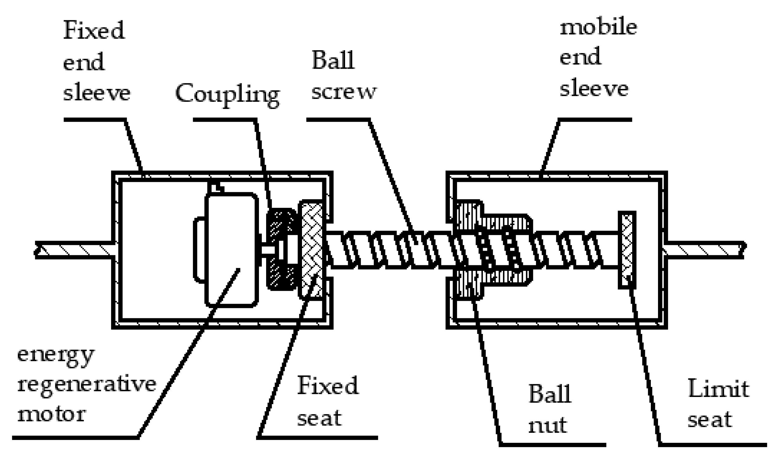
3.4.1. Design of Mechanical Structure of Energy Regenerative Actuator

The commonly used mechanical structures of energy regenerative suspension mainly includes rack pinion type [20], crank linkage type [21], linear motor type [22] and ball screw type. The rack pinion type, crank linkage type and ball screw type all convert the linear up-and-down motion of the suspension into the rotational motion of the motor rotor through a specific mechanical structure, thus, driving the motor to generate electricity, which is finally stored and reused. The linear motor type converts the vertical vibration energy of the suspension directly into electrical energy, and also converts the electrical energy into linear motion and provides damping force to the suspension system. The rack pinion structure is not recommended, because the rack and pinion can easily break when the road excitation impact is too large, resulting in failure of the energy regenerative suspension. Crank linkage structure involves two major problems: one is the low efficiency of energy recovery, as most of the energy is dissipated in the form of heat, and the energy recovery effect is not good; the second major problem is the crank linkage mechanism occupies a large space, and is not easy to install. Among the commonly used mechanical structures of energy regenerative suspension, the ball screw type energy recovery and active control process need to be through the ball screw mechanism for vertical motion and rotary motion conversion, due to the existence of friction between the parts in the mechanical structure of the transmission process, leading to energy loss and output damping force accuracy. The linear motor type does not need to be through the mechanical structure of the transmission to achieve energy recovery and active control force output, so the efficiency of energy recovery and control damping force accuracy is higher than the ball screw type. However, there are two major problems with the linear motor compared to the rotary motor used in the ball screw type: one problem is that the linear motor has low rated power and the energy consumption in providing the same damping force is greater than that of the rotary motor and the second problem is that the linear motor is expensive and has high manufacturing costs. Therefore, this paper used the ball screw type structure as the mechanical structure of the energy regenerative actuator.

The simple mechanical structure of the energy regenerative actuator is shown in Figure 4, where the fixed end sleeve is used to connect the actuator to the body and the mobile end sleeve is used to connect the actuator to the wheels. The coupling is used to connect the ball screw and the energy regenerative motor, the fixed seat is used to connect the fixed end sleeve, the ball nut is used to connect the mobile end sleeve, and it works together with the ball screw to translate the vertical vibration of the suspension and the rotational motion of the motor rotor. The limit seat is used to limit the motion range of the ball screw mechanism to ensure that the motion range of the actuator is within the permitted dynamic travel of the suspension (±0.1 m).

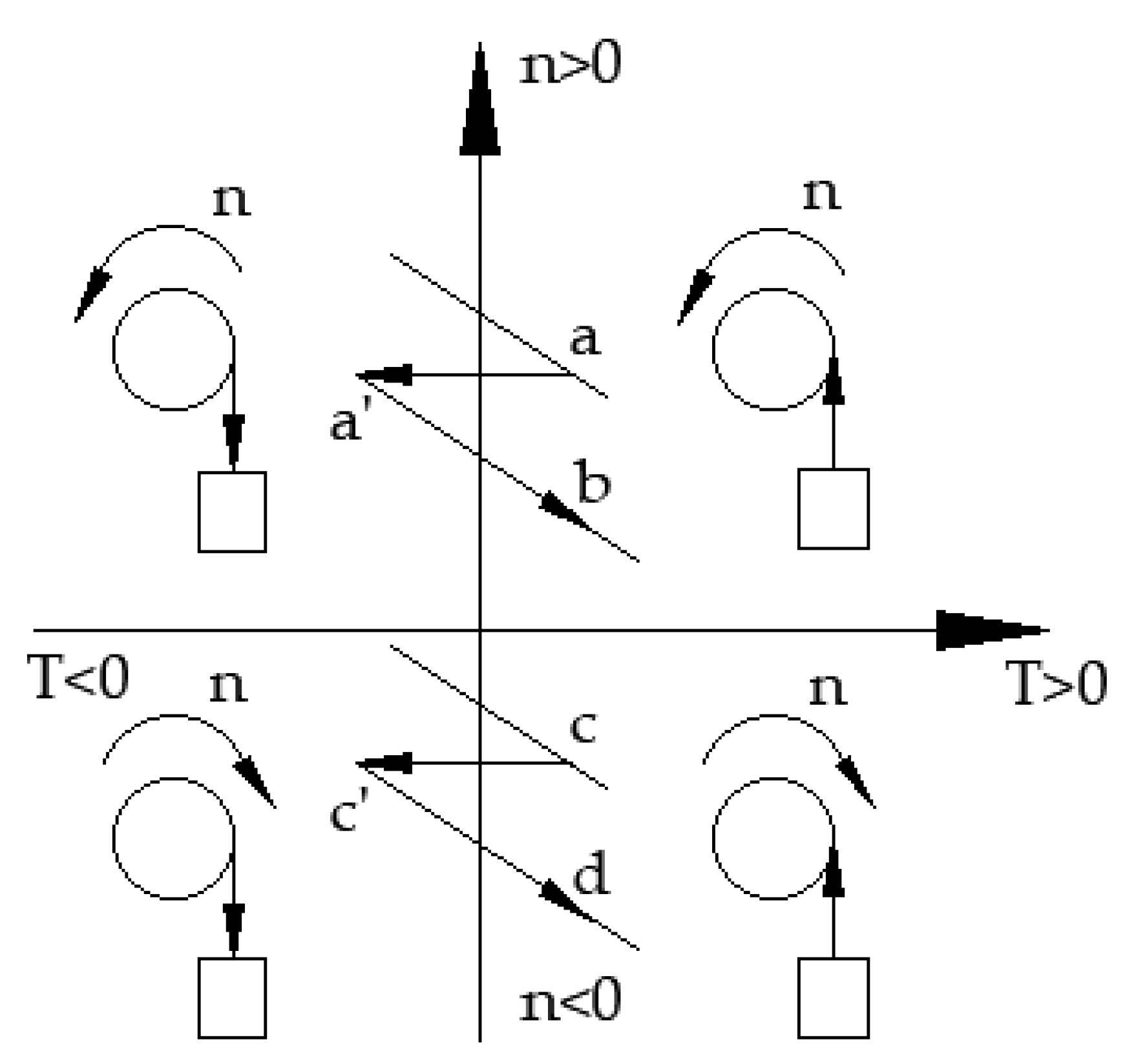
3.4.2. Four-Quadrant Operation Principle of Energy Regenerative Motor

The core device of the energy regenerative actuator is the energy regenerative motor, and the overall concept of the work of the actuator can be obtained according to the operation law of the energy regenerative motor [23]. Figure 5 below shows the four-quadrant operation diagram of the energy regenerative motor.

Define the torque T and speed n, and choose the counterclockwise direction as the positive direction of speed and torque. The coordinate system is divided into four quadrants by the direction of speed and torque. The first quadrant indicates that the motor lifts the weight, and the fourth quadrant indicates that the motor drops the weight. In the fourth quadrant, the speed is n < 0, and the motor has to output counterclockwise torque T to resist the falling of the weight while rotating clockwise at a certain speed, and the motor is in generator mode at this time. In the third quadrant, the weight cannot fall naturally due to insufficient gravity, so the motor is required to provide output torque for the weight to fall, at which time T < 0 and n < 0. In the second quadrant, the motor will not remain stable no matter where it is operating, but there can be such a state in the transition phase, for example, when the motor is operating in the first quadrant, it wants to make the rotational speed at that time from point a rapidly to point b. If the inertia of the motor is taken into account, this inertia will cause the speed to remain in a continuous process of change. Therefore, in the transition phase, the speed of the motor will remain constant for a moment, that is, it will move from point a to point a’ in the second quadrant, and the motor will work in the generator state, after which the motor will start to decelerate and finally run stably at point b. Observe in the fourth quadrant at point c, which concerns the motor running at low speed, it is hoped that the motor can quickly rise to point d. As in the above analysis, the operation of the motor will change along the operation state of c → c’ → d, so that the motor movement state will also appear in the third quadrant during the transition process, so that the motor can be in two modes of motor and generator switching changes.

In summary, when the motor running state is in the first and third quadrants, the motor works in the motor state, and, at this time, the control motor through the ball screw mechanism output active control force can attenuate vibration. When the motor running state is in the second and fourth quadrants, the motor works in the generator state, the actuator is in the follower state, and, at this time, the motor can generate damping force for passive damping and can recover the energy generated by vibration.

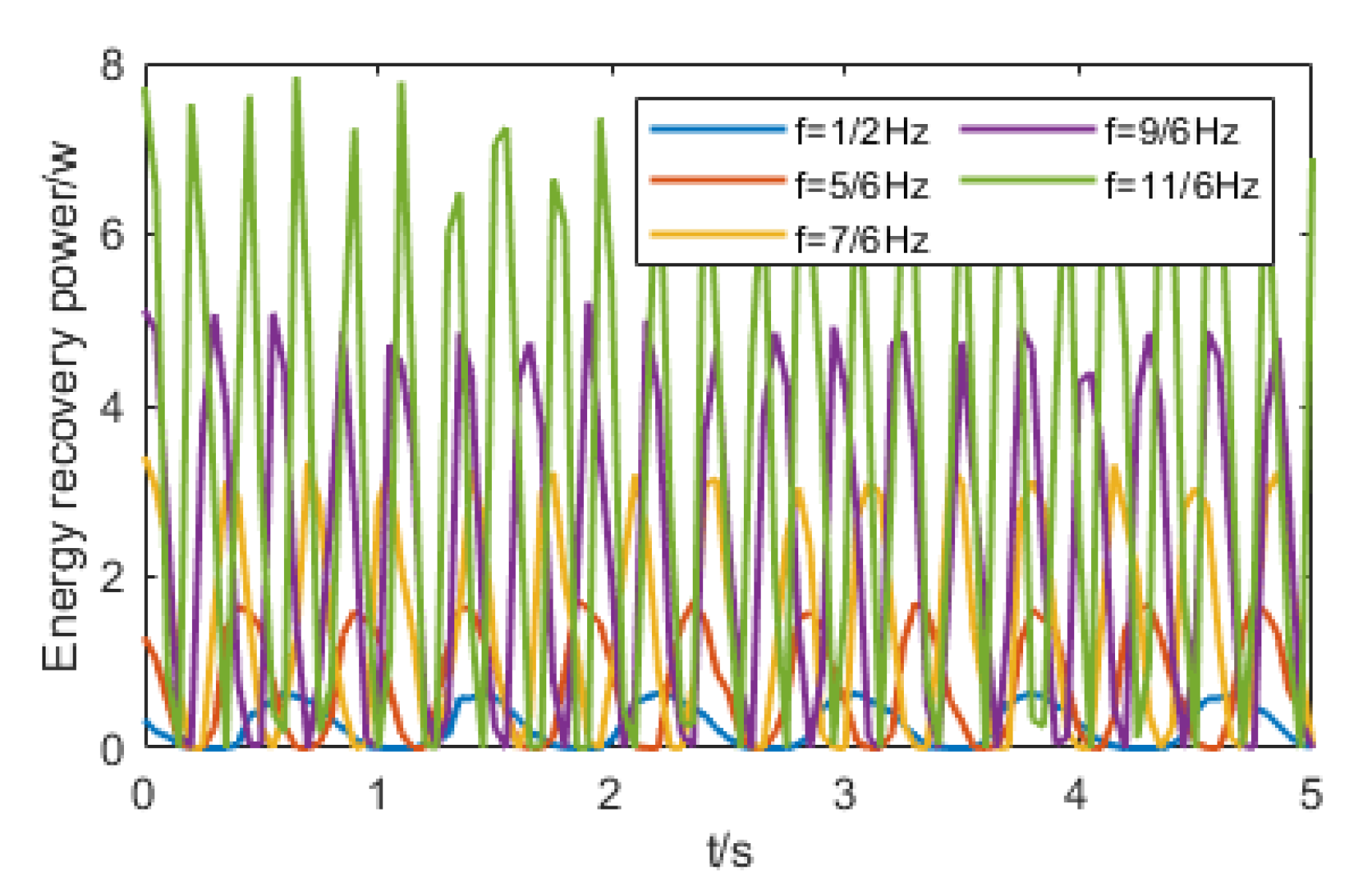
3.4.3. Mathematical Model for Energy Recovery

During the driving process of the vehicle, road excitation will cause suspension vibration through the ball screw mechanism drive, so that the energy recovery motor rotor rotation, known rotor angular velocity ω, rotor speed n and suspension vibration speed $v_i$ relationship are as follows (8), (9), shown in the formula.

$$\omega =2\pi n$$

(8)

$$n=\frac{v_i}{l}$$

(9)

where l is the ball screw lead, expressing the ball screw rotating a single revolution, the displacement of the ball nut moving and $v_i$ is the suspension vibration speed of each wheel, where the suspension vibration speed is defined as: $v_i={\dot{z}}_{bi}-{\dot{z}}_i$, i = 1, 2, 3, 4.

For an ideal ball screw actuator [24,25], the following equation is available.

$$T=\rho I$$

(10)

$$F_d=T\cdot \frac{2\pi }{l}=\frac{2\pi \rho I}{l}$$

(11)

where T is the motor torque, $\rho$ is the electromagnetic torque constant of the energy regenerative motor, and I is the armature circuit current of the energy regenerative motor.

The equivalent circuit of the feeder motor is shown in Figure 6 below, where U is the voltage across the energy regenerative motor, r is the internal resistance of the energy regenerative motor, L is the inductance of the energy regenerative motor, E is the induced electric potential of the energy regenerative motor and R is the equivalent resistance of the energy regenerative circuit.

As shown in Figure 6a, when the energy recovery circuit in the energy recovery actuator works, the energy recovery motor load is the energy recovery circuit. At this time, the energy regenerative motor is a generator and the energy recovery motor supplies power to the energy recovery circuit, at this time. At this point, the induced potential and armature circuit current of the energy regenerative motor are shown in the following equation.

$$E=\rho \cdot \omega$$

(12)

$$I=\frac{E}{(R+r)}$$

(13)

Coupling (8), (9), (11), (12), (13), the electromagnetic damping force $F_d$ and the electromagnetic damping coefficient c are obtained as follows:

$$F_d=\frac{4{\pi }^2{\rho }^2}{l^2(R+r)}\cdot v_i$$

(14)

$$c=\frac{4{\pi }^2{\rho }^2}{l^2(R+r)}$$

(15)

From the above Equations (14) and (15) it can be seen, at this time, that the electromagnetic damping force is only related to the suspension vibration speed and resistance value, the damping coefficient is only related to the resistance value, so when the energy recovery circuit works, the actuator only plays a passive damping and energy recovery effect. The energy recovery power as shown in Equation (16).

$$P=\frac{E^2}{R}=\frac{4{\pi }^2{\rho }^2}{l^{2}R}\cdot v_i^2$$

(16)

3.4.4. Mathematical Model for Active Control

As shown in Figure 6b, when the active control circuit in the energy recovery actuator works, the load of the energy recovery motor is the car battery, and the car battery supplies power to the energy recovery motor. St this time the active control force is shown in Equation (11), and the voltage U at both ends of the energy recovery motor is shown in Equation (17).

$$U=L\cdot \frac{dI}{dt}+rI+E$$

(17)

where t is time.

From Equation (11), it can be seen that the magnitude of the active control force is proportional to the motor armature circuit current, so the actual current in the armature circuit can be controlled so as to be similar to the ideal current given by the controller, by controlling the voltage at both ends of the car battery input to the energy recovery motor, thus, achieving an actual control force $F_d$ that is similar to the ideal control force $F_0$. A Laplace transformation of Equation (17) yields Equation (18).

$$\frac{I(s)}{U(s)-E(s)}=\frac{1}{Ls+r}$$

(18)

Currently, the actuator current closed-loop controls on the market mainly use the PID control algorithm [26] This paper used the fractional order PID control algorithm to achieve the motor current closed-loop control, combined with the above Equation (18). The design control circuit’s specific principle is shown in Figure 7 below.

3.4.5. Analysis of the Relationship between Key Parameters and Performance of Actuator

From the Equations (14) and (15), it can be seen that the electromagnetic damping force and energy recovery power is related to the electromagnetic torque constant and ball screw lead in the actuator. Under the condition of constant suspension vibration speed, the larger the electromagnetic torque constant, the smaller the ball screw lead, the larger the electromagnetic damping force and the higher the energy recovery power. However, combined with Equation (11) and the formula $P_1{=F}_d·v$, where $P_1$ is the power of the active control force, the formula of the active control force work power is as follows:

$$P_1=\frac{2\pi \rho I}{l}\cdot v_i$$

(19)

As can be seen from the above equation, the greater the electromagnetic torque constant and the smaller the ball screw guide, the greater the power consumed by the active control force doing work. Therefore, when designing the energy regenerative actuator, the electromagnetic torque constant and the ball screw guide should be determined by considering the energy recovery and the power consumed, so as to reduce the energy consumption, while ensuring the vibration damping effect.

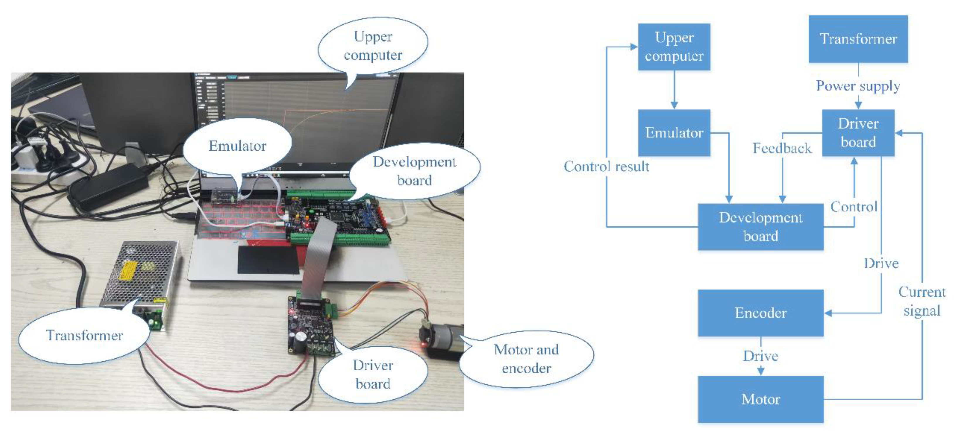
3.4.6. Digital Implementation of Control Circuits

The conventional PID control law is shown in Equation (20):

$$u(t)=K_{p}e(t)+K_i{\displaystyle {\int }_0^{t}e(t)dt}+K_d\frac{de(t)}{dt}$$

(20)

Fractional order PID control is similar to PID control, except that differential control and integral control are turned into $D^{\mu }$ and $I^{\lambda }$ of adjustable order, and the control law of fractional order PID is [27,28,29]:

$$u(t)=K_{p}e(t)+K_i\cdot {}_{t_0}D{}_t^{-\lambda }e(t)+K_d\cdot {}_{t_0}D{}_t^{\mu }e(t)$$

(21)

where ${}_{t_0}{}^{}D{}_t^{-\lambda }$ and ${}_{t_0}{}^{}D{}_t^{\mu }$ are fractional order calculus operators, where λ and μ must be real numbers, t is the independent variable, and $t_0$ is the lower bound of the variable, and where the independent variable t is time. The uniform fractional order calculus operator ${}_{t_0}{}^{}D{}_t^{\alpha }$ is defined as:

$${}_{t_0}D{}_t^{\alpha }f(t)=\{\begin{array}{l}{\displaystyle {\int }_{t_0}^{t}f(\tau )d{\tau }^{-\alpha },\alpha <0}\\ f(t),\alpha =0\\ \frac{d^{\alpha }}{d{t}^{\alpha }}f(t),\alpha >0\end{array}$$

(22)

where α is the fractional order.

Equations (20) and (21) are generally discretized during the design of the test controller, where the equation for designing the PID controller is shown below:

$$u_k=K_p{e}_k+K_i{\displaystyle \sum _{j=o}^k{e}_j}+K_d(e_k-e_{k-1})$$

(23)

Similarly, the design of the test controller requires the use of a discretized fractional order PID formula, which, in this paper, was designed using the $\mathrm{Gr}\ddot{\mathrm{u}}\text{nwald-Letnikov}$ formula, the differential of which is defined by the following equation:

$${}_{t_0}{}^{GL}D{}_t^{\alpha }f(t)=\underset{h\to 0}{\lim }\frac{1}{h^{\alpha }}{{\displaystyle \sum _{j=0}^{[(t-t_0)/h]}(-1)}}^j\left(\begin{array}{c}\alpha \\ j\end{array}\right)f(t-jh)$$

(24)

where $[(t-t_0)/h]$ represents the nearest integer of $(t-t_0)/h$; $\left(\begin{array}{c}\alpha \\ j\end{array}\right)$ is the coefficient of binomial; The integral definition simply changes the fractional order $\alpha$ in the differential equation to $-\alpha$. Simultaneous upper Equations (21) and (24) can be obtained:

$$u(t)=K_{p}e(t)+K_i\underset{h\to 0}{\lim }\frac{1}{h^{-\lambda }}{\displaystyle \sum _{j=0}^{[(t-t_0)/h]}{c}_{j}e(t-jh)}+K_d\underset{h\to 0}{\lim }\frac{1}{h^{\mu }}{\displaystyle \sum _{j=0}^{[(t-t_0)/h]}{d}_{j}e(t-jh)},(\lambda ,\mu >0)$$

(25)

where, $c_j$ and $d_j$ are integral term coefficients and differential term coefficients respectively. Fractional calculus equations are generally realized by numerical approximation. Two coefficients can be approximated by using the following recursive equation:

$$c_j=[1-(1-\lambda )/j]c_{j-1},c_0=1,j=1,2,3\cdots$$

(26)

$$d_j=[1-(1+\mu )/j]d_{j-1},d_0=1,j=1,2,3\cdots$$

(27)

When the calculation step h selected in the above Equation (19) is small enough, the limit calculation operation in the above formula can be ignored, and $t_0$ = 0 in this paper, the following Equation (28) can be obtained:

$$u(t)=K_{p}e(t)+K_i{h}^{\lambda }{\displaystyle \sum _{j=0}^{[t/h]}{c}_{j}e(t-jh)}+K_d{h}^{-\mu }{\displaystyle \sum _{j=0}^{[t/h]}{d}_{j}e(t-jh)},(\lambda ,\mu >0)$$

(28)

From Equation (28) above, the discretization equation for fractional order PID can be derived as follows:

$$u_k=K_p{e}_k+K_i{h}^{\lambda }{\displaystyle \sum _{j=0}^k{c}_j{e}_{k-j}}+K_d{h}^{-\mu }{\displaystyle \sum _{j=0}^k{d}_j{e}_{k-j}},(\lambda ,\mu >0),(k=1,2,3\cdots )$$

(29)

In order to describe the fractional order PID control circuit more clearly, the fractional order PID (FOPID) control flow of the current is described in Algorithm 1.

Algorithm 1: FOPID

Input:$k_p{,k}_i{,k}_d,\lambda ,\mu$, Ideal current value $I_0$. Output: Actual current value $I$.

1: Limiting current amplitude to prevent integral saturation: If $I \ge$ maximum motor operating current $I_{\max }$, $I=I_{\max }$. Else if $I \le$ minimum motor operating current $I_{min}$, $I=0$. 2: Calculation of error values: $e_k{=I}_0-I$. 3: Setting of current accuracy: If $-5\mathrm{mA}\le e_k\le 5\mathrm{mA}$,$e_k=0$. 4: For j=0: k − 1. 5: Update the binomial coefficients $c_j$ and $d_j$ from Equations (20), (21). 6: Updating the input motor voltage U from Equation (23). 7:   $e_{k-j-1}{=e}_{k-j}$. 8: End for. 9: Return I.

4. Experimental Study of Energy Regenerative Actuators

4.1. Experimental Study of Energy Regenerative

The electromagnetic torque constant is the most important performance parameter of the energy recovery motor. The purpose of the energy recovery test is to estimate the electromagnetic torque constant of the used energy recovery motor and to provide a parameter basis for the subsequent simulation study, which can be obtained from Equation (16) as follows:

$$\rho =\frac{l}{2\pi v_i}\cdot \sqrt{PR}$$

(30)

From Equation (30), the equation for estimating the electromagnetic torque constant is given by the following equation:

$${\rho }_f=\frac{l}{2\pi {\overline{v}}_i}\cdot \sqrt{\overline{P}R}$$

(31)

where ${\rho }_f$ represents the experimentally calculated value of the electromagnetic torque constant, ${\overline{v}}_i$ represents the mean suspension vibration speed and $\overline{P}$ represents the mean energy recovery power.

The type of feeder motor used for the test was a DC brushless motor, and the ball screw mechanism used had a lead of 0.02 m. Simple harmonic vibration of different frequencies was used to simulate the suspension vibration, setting the amplitude of simple harmonic vibration to 0.02 m and the initial phase to 0. The frequencies of simple harmonic vibration were 1/2 Hz, 5/6 Hz, 7/6 Hz, 9/6 Hz and 11/6 Hz. The overall structure and workflow of the experimental rig is shown in Figure 8a below. The vibration platform controlled the actuator placement rack according to the set parameters for simple harmonic vibration, and the actuator placement rack drove the ball screw energy recovery actuator to achieve energy recovery, and the ball screw energy recovery actuator is shown in Figure 8b below. The energy recovery parameters were measured by the measurement module. The measurement module was connected to a 50 Ω resistor as the equivalent resistance of the energy recovery circuit, and a sample of the measured data was displayed and plotted on the upper computer with the sampling period set to 0.05 s. The test results are shown in Figure 9 and

Table 1. Energy recovery test data.

Vibration Frequency/Hz	Mean Vibration Speed/ $m\mathbf{·}{\mathbf{s}}^{-1}$	Power Averages/W	Values of Electromagnetic Torque Constants
1/2	0.0401	0.2637	0.2879
5/6	0.0672	0.7412	0.2884
7/6	0.0927	1.4553	0.2928
9/6	0.1204	2.3707	0.2878

below.

According to the test results, as the vibration frequency increased, the average value of the suspension vibration speed and the average value of the energy recovery power also increased, while the value of the electromagnetic torque constant fluctuated very little, which proved that the electromagnetic torque constant estimated by Equation (31), combined with the test results, was close to the actual value. The electromagnetic torque constant at each vibration frequency was taken as the average value, and the electromagnetic torque constant of the energy recovery motor used was about 0.2885.

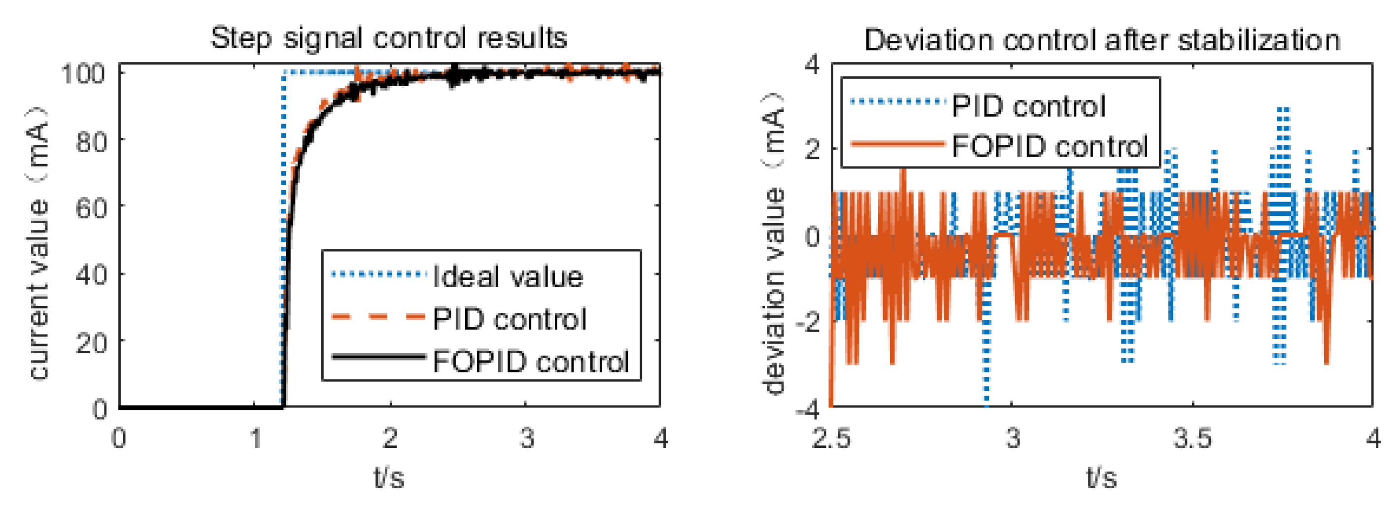
4.2. Experimental Study of Control Circuits

In this paper, the STM32-F407 development board was used as the control algorithm carrier and Keil software was used in the upper computer to write the PID and fractional order PID control programs and set the initial parameters of the controller. The program was loaded into the development board through the emulator, the development board controlled the drive board, the transformer supplied power to the drive board, the drive board drove the motor through the encoder, and the current sampling circuit on the drive board collected the current signal in the motor and fed it back to the development board. The development board controlled the current level in the motor in real time and fed the control result to the upper computer for display. The test equipment and test process are shown in Figure 10.

After several test adjustments, for the motor used in the test, the parameters for PID control were taken to be $k_p$ = 1.5, $k_i$ = 3.5, $k_d$ = 0.2 and for fractional order PID control $k_p$ = 0.1, $k_i$ = 2, $k_d$ = 0.1, λ = 0.4, μ = 0.7. Figure 11 below shows the test results for PID and fractional order PID for current with step signals.

As shown in Figure 11, the PID and fractional order PID control reached the stable value (about 2.5 s) almost simultaneously, and the regulation time was basically the same. The control effect of both the PID control circuit and the fractional order PID control circuit could meet the requirements of the actuator current control, which proved the feasibility of the actuator control circuit. After the control was stable, the fractional order PID control effect was better than the PID control, which proved the superiority of the designed fractional order PID control circuit.

5. Principle of Active Control of the Whole Vehicle

The principle of the whole vehicle active control of the suspension system is shown in Figure 12. The suspension system outputted the body mass acceleration signal ${\ddot{z}}_b$ and the given value 0 to generate the deviation signal e(t) to the controller, which was controlled by four fractional order PID controllers to realize the output of the ideal control forces $F_{01}$,$F_{02}$,$F_{03}$ and $F_{04}$ of the suspension on each wheel respectively. The control circuit controlled the actuator to output the actual control forces $F_{d1}$,$F_{d2}$,$F_{d3}$ and $F_{d4}$. The parameter tuning algorithm optimized the objective function to achieve the parameter tuning of the four fractional order PID controllers.

5.1. Fractional Order PID Controller Simulation Model

The transfer function of a fractional order PID controller is shown in the following equation:

$$G(s)=K_p+K_i/s^{-\lambda }+K_d{s}^{\mu }$$

(32)

The simulation procedure used a modified Oustaloup filter [30] to implement the approximation of the fractional order calculus operator $s^{\alpha }$, and there were several main steps in constructing the fractional order calculus operator.

(1) Determination of the filter order N and the approximate frequency band [$w_b$, $w_h$].

(2) Calculate the zero poles $w_k^{\prime }$ and $w_k$, as shown in Equations (33) and (34):

$$w_k^{\prime }=w_b{w}_{\mu }^{(2k-1-\alpha )/N},w_k=w_b{w}_{\mu }^{(2k-1+\alpha )/N}$$

(33)

$$k=w_h^{\alpha },w_{\mu }=\sqrt{w_h/w_b}$$

(34)

(3) Finally, complete the approximation to the fractional order calculus operator, as shown in Equation (35).

$$s^{\alpha }={(\frac{d{w}_h}{b})}^{\alpha }(\frac{d{s}^2+b{w}_{h}s}{d(1-\alpha )s^2+b{w}_{h}s+d\alpha }){\displaystyle \prod _{k=1}^N\frac{s+w_k^{\prime }}{s+w_k}}$$

(35)

The above equation had to be satisfied with α (0< α <1); in general, the approximate frequency band was set to [0.001,1000], the filter order N was 5, and the weighting parameters were chosen as b = 10, d = 9 to meet the accuracy requirements. Improved Oustaloup filters that approximated the fractional order calculus operators $s^{-\lambda }$ and $s^{\mu }$ were designed from Equation (35) above.

5.2. Design of Objective Function

Before the controller parameters were adjusted, the main problem is to clarify the optimization objectives to be faced by the controlled system. The purpose of the active control of the suspension was to improve comfort of ride, driving safety and handling stability of the vehicle, and the design objective function is shown below:

(1) The vehicle’s center of mass acceleration ${\ddot{z}}_b$, roll angular acceleration $\ddot{\varphi }$ and pitching angular acceleration $\ddot{\theta }$ were chosen to characterize the smoothness of the ride.

(2) Four suspension dynamic deflections ${(z}_{b_1}{-z}_1{),(z}_{b_2}{-z}_2{),(z}_{b_3}{-z}_3)$ and ${(z}_{b_4}{-z}_4)$ were selected to characterize driving safety.

(3) Four dynamic tire loads $k_1{(z}_1{-q}_1{),k}_2{(z}_2{-q}_2{),k}_3{(z}_3{-q}_3)$ and $k_4{(z}_4{-q}_4)$ were selected to characterize handling stability.

The above parameters were normalized to design the objective function, as shown in the following equation:

$$\begin{array}{c}J={\rho }_1[\frac{rms({\ddot{z}}_b)}{rms{({\ddot{z}}_b)}_p}]+{\rho }_2[\frac{rms(\ddot{\varphi })}{rms{(\ddot{\varphi })}_p}]+{\rho }_3[\frac{rms(\ddot{\theta })}{rms{(\ddot{\theta })}_p}]+{\rho }_4[\frac{rms(z_{b1}-z_1)}{rms{(z_{b1}-z_1)}_p}]+{\rho }_5[\frac{rms(z_{b2}-z_2)}{rms{(z_{b2}-z_2)}_p}]+{\rho }_6[\frac{rms(z_{b3}-z_3)}{rms{(z_{b3}-z_3)}_p}]\\ +{\rho }_7[\frac{rms(z_{b4}-z_4)}{rms{(z_{b4}-z_4)}_p}]+{\rho }_8[\frac{rms(z_1-q_1)}{rms{(z_1-q_1)}_p}]+{\rho }_9[\frac{rms(z_2-q_2)}{rms{(z_2-q_2)}_p}]+{\rho }_{10}[\frac{rms(z_3-q_3)}{rms{(z_3-q_3)}_p}]+{\rho }_{11}[\frac{rms(z_4-q_4)}{rms{(z_4-q_4)}_p}]\end{array}$$

(36)

where: the subscript p represents the passive suspension indicators and rms(.) denotes the root mean square value of each indicator, which was designed to make the performance indicators dimensionless and facilitate the selection of weighting factors. The values ${\rho }_1~{\rho }_{11}$ are weighting factors, due to the different importance of each indicator in the suspension system. Due to the coupling between the acceleration of the body center of mass vertical vibration, the acceleration of the roll angular, the acceleration of the pitching angular, the dynamic deflection of the suspension and the dynamic tire load, when some of these indicators needed to achieve a better value, the degree of optimization of some other indicators had to be sacrificed. Therefore, ${\rho }_1~{\rho }_{11}$ were set in the interval of (0,1), ${\displaystyle \sum }_{i=1}^{11}{\rho }_i=1$, according to the order of optimization of each index and then combined with the constraints to determine the required optimization index of the weighting factor ${\rho }_1~{\rho }_{11}$ chosen. The large ${\rho }_1~{\rho }_3$ were selected to improve the smoothness of the car; the suspension dynamic deflection could be used as the optimization index of sacrifice, so the smaller ${\rho }_4~{\rho }_7$ were selected to ensure the optimization effect of driving smoothness and handling stability, but were not too small to ensure that the suspension dynamic deflection did not exceed the permissible range (generally taken as ±0.1 m) to avoid damage to the suspension to affect driving safety; were selected to ensure the optimization effect of driving smoothness and handling stability, but were not too small to ensure that the suspension dynamic deflection did not exceed the permissible range (generally taken as ±0.1 m) to avoid damage to the suspension to affect driving safety; ${\rho }_8~{\rho }_{11}$ could be selected as larger values to ensure the optimized effect of handling stability. In summary and after several simulations,${\rho }_1$ = ${\rho }_2$ = ${\rho }_3$ = 0.16, ${\rho }_4$ = ${\rho }_5$ = ${\rho }_6$ = ${\rho }_7$ = 0.05, ${\rho }_8$ = ${\rho }_9$ = ${\rho }_{10}$ = ${\rho }_{11}$ = 0.08.

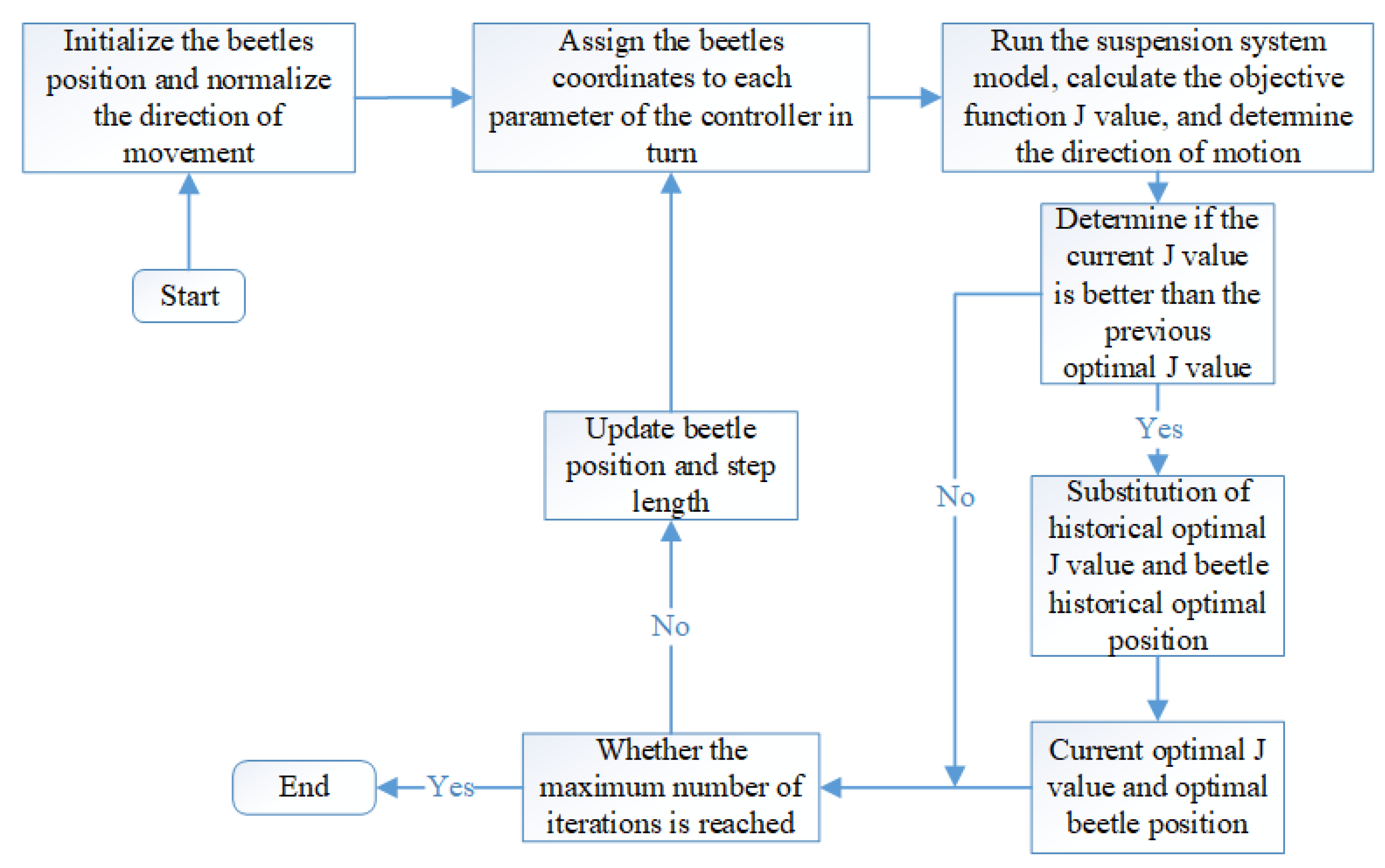
5.3. Beetle Antenna Search Algorithm

Although the fractional order PID controller would improve the control ability of the system to a certain extent, it was much more difficult to adjust the parameters than the PID controller because there were two more parameters, so this paper adopted a new bionic algorithm, the Beetle Antenna Search Algorithm (BAS), to realize the parameter adjustment of the fractional order PID controller [31]. The algorithm transformed the N-parameter optimization problem into a problem of beetle foraging in N-dimensional space. The value of the evaluation index function J was equivalent to the concentration of the food, and the value of the parameter obtained by the search for the best was equivalent to the location coordinates of the beetle. The iterative process of the Beetle Antennae Search Algorithm can be presented as follows:

First, the position information of Beetle was initialized ${X(x}_1{,x}_2{,\dots ,x}_N{)}^T$. The N dimensional random vector $\overrightarrow{d}$ was established to represent the movement direction of beetle:

$$\overrightarrow{d}=\frac{rands(N,1)}{\Vert rands(N,1)\Vert }$$

(37)

where rands(.) refers to the random matrix function;

The beetle can choose the moving direction and update the next position by judging the food concentration on the coordinates of the left and right antennae. Equation (38) was used to determine the position of the left and right antennae of beetle, and Equation (39) was used to update the position of beetle.

$$\{\begin{array}{l}{X}_r=X+l_0\cdot \overrightarrow{d}\\ X_l=X-l_0\cdot \overrightarrow{d}\end{array}$$

(38)

$$X_{t+1}=X_t+{\delta }_t\cdot \overrightarrow{d}\cdot sign[J(X_r)-J(X_l)]$$

(39)

where $l_0$ represents the distance between beetle and antennae, $X_r$ is the right antennae position of beetle, $X_l$ is the left antennae position of beetle; t represents the current iteration number; $J(.)$ is the value of the objective function J; ${\delta }_t$ represents the search step at the t iteration, calculated by Equation (40), sign(.) is a symbolic function, calculated by Equation (41).

$${\delta }_{t+1}={\delta }_t\cdot eta$$

(40)

$$sign(x)=\{\begin{array}{l}1,x>0\\ 0,x=0\\ -1,x<0\end{array}$$

(41)

The current minimum objective function J value was compared with the historical minimum objective function J value, and the best J value and position were updated, and the best position coordinates were selected as the best parameters of the fractional order PID controller. As the beetle moved closer to the food, the step size needed to be decayed in order to improve the convergence speed. In Equation (40) eta is the step size decay coefficient, which was generally taken as 0.95. After updating the step size, the beetle coordinates were updated and the next iteration was carried out until the maximum number of iterations was reached. The highest concentration of food in the beetle foraging process was the optimal objective function value, and the coordinates of the location with the highest food concentration were the final optimal parameters obtained.

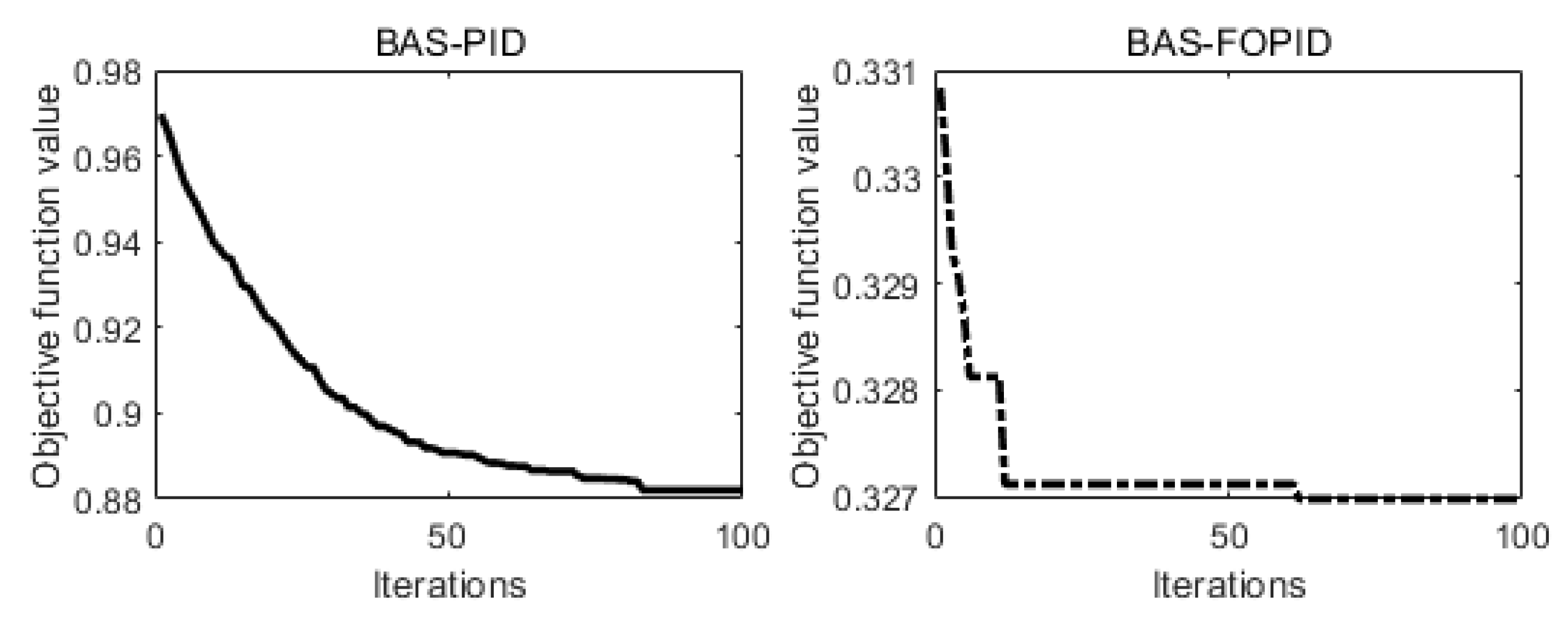
5.4. Parameter Adjustment Process and Results

Since each fractional order PID controller had five adjustable parameters, set the solution space dimension Dim = 20, the position information $X$ was: ($K_{p1}$,$K_{i1}$,$K_{d1}$,${\lambda }_1$,${\mu }_1$,$K_{p2}$,$K_{i2}$,$K_{d2}$,${\lambda }_2$,${\mu }_2$,$K_{p3}$,$K_{i3}$,$K_{d3}$,${\lambda }_3$,${\mu }_3$,$K_{p4}$,$K_{i4}$,$K_{d4}$,${\lambda }_4$,${\mu }_4{)}^T.$ Consider the parameter setting speed and accuracy, set the number of beetles S = 10, maximum number of iterations M = 100, initial step size ${\delta }_0$ = 2, step length attenuation factor eta = 0.95, The distance between the left and right whiskers of beetle l = 2. In addition, in order to shorten the search time of the algorithm and improve the search accuracy, it was necessary to determine the hunting space of beetle. According to experience, the upper bound $U_H$ was [1000,1000,500,1,1,1000,1000,500,1,1,1000,1000,500,1,1,1000,1000,500,1,1] and the lower bound $U_L$ was [0,0,0,0,0,0,0,0,0,0,0,0,0,0,0,0,0,0,0,0].

Similarly, for PID controller parameter tuning, set solution space dimension Dim = 12, the position information $X$ was ($K_{p1}$,$K_{i1}$,$K_{d1}$,$K_{p2}$,$K_{i2}$,$K_{d2}$ ,$K_{p3}$,$K_{i3}$,$K_{d3}$,$K_{p4}$,$K_{i4}$,$K_{d4}{)}^T$, $U_H$ was [1000,1000,500,1000,1000,500,1000,1000,500,1000,1000,500] and the $U_L$ was [0,0,0,0,0,0, 0,0,0,0,0,0], and other parameters were the same. Special attention should be paid to the fact that the smaller the evaluation index function value was in this paper, the higher the food concentration was, so Equation (39) should be changed to the following equation:

$$X_{t+1}=X_t-{\delta }_t\cdot \overrightarrow{d}\cdot sign[J(X_r)-J(X_l)]$$

(42)

Figure 13 shows a flow chart of PID and fractional order PID parameter adjustment using the Beetle Antenna Search algorithm.

The controller parameters were obtained by using the Beetle Antennae Search Algorithm to find the optimal controller parameters several times, as shown in

Table 2. Controller parameters adjustment results.

Parameter Name	Control Method		Parameter Name	Control Method
	BAS-PID	BAS-FOPID		BAS-PID	BAS-FOPID
$K_{p1}$	807.4029	554.8152	$K_{p3}$	540.1069	666.2706
$K_{i1}$	936.2899	421.1504	$K_{i3}$	83.3911	749.3380
$K_{d1}$	228.4008	545.0502	$K_{d3}$	64.5269	446.2735
${\lambda }_1$	1	0.4645	${\lambda }_3$	1	0.2909
${\mu }_1$	1	0.1892	${\mu }_3$	1	0.3609
$K_{p2}$	788.5277	351.4805	$K_{p4}$	521.3142	589.0160
$K_{i2}$	164.5138	982.9772	$K_{i4}$	93.6735	705.4344
$K_{d2}$	444.9254	113.6506	$K_{d4}$	151.8317	254.5784
${\lambda }_2$	1	0.1577	${\lambda }_4$	1	0.2135
${\mu }_2$	1	0.2045	${\mu }_4$	1	0.2033

below.

Figure 14 below shows the objective function optimization curve of each controller under the BAS algorithm.

From Figure 14, it can be seen that the objective function of fractional order PID controller reached the optimal value when the number of iterations was 62, while the objective function of PID controller reached the optimal value when the number of iterations was 83. In addition, the optimal value of the objective function under fractional order PID control was 0.3270, which was obviously smaller than the optimal value of the objective function under PID control of 0.8821, proving that the objective function optimization of the fractional order PID controller was better than that of the PID controller.

6. Performance Simulation Analysis of Complete Vehicle Suspension System

MATLAB and Simulink were used to model the passive suspension system of the whole vehicle, the active suspension system under PID control and fractional order PID control, and the actuator. In this paper, with reference to the parameters of the Volkswagen Jetta sedan, the parameters of the whole vehicle suspension system were taken as shown in

Table 3. The whole vehicle suspension system parameters table.

Parameter	Value	Parameter	Value
$m_b/\mathrm{kg}$	1440	$k_1{,k}_2{,k}_3{,k}_4/\mathrm{N}·{\mathrm{m}}^{-1}$	190,000
$m_1{,m}_2/\mathrm{kg}$	40	$l_1/\mathrm{m}$	1.2
$m_3{,m}_4/\mathrm{kg}$	45	$l_2/\mathrm{m}$	1.5
$K_1{,K}_2/\mathrm{N}·{\mathrm{m}}^{-1}$	17,000	$l_3{,l}_4/\mathrm{m}$	0.75
$K_3{,K}_4/\mathrm{N}·{\mathrm{m}}^{-1}$	22,000	$I_x/\mathrm{kg}·{\mathrm{m}}^2$	2440
$c_1{,c}_2{,c}_3{,c}_4/\mathrm{N}·\mathrm{s}·{\mathrm{m}}^{-1}$	1500	$I_y/\mathrm{kg}·{\mathrm{m}}^2$	380
$\rho$	0.2885	$r/\Omega$	30
$L/\mathrm{H}$	0.3	$l/\mathrm{m}$	0.02

below.

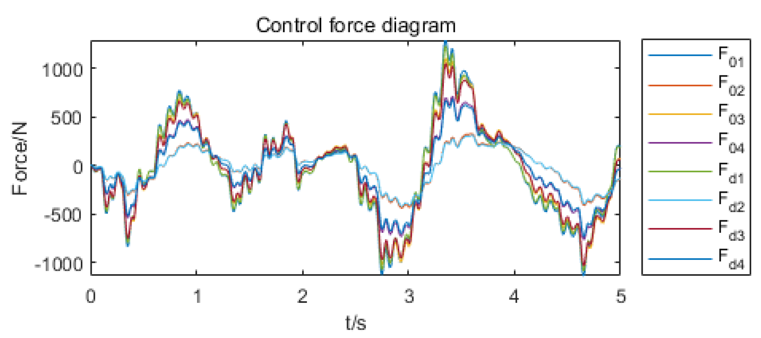
6.1. Actuator Control Force Simulation Analysis

Figure 15 below shows the actual control force output by each wheel actuator compared to the ideal control force under the fractional order PID control circuit.

In Figure 15, $F_{01}$, $F_{02}$, $F_{03}$ and $F_{04}$ were the ideal control forces output under each fractional order PID control, and $F_{d1}$, $F_{d2}$, $F_{d3}$ and $F_{d4}$ were the actual control forces output under each actuator control circuit control. It can be seen from Figure 12 that the actual control force curves of each were very close to the ideal force curves, where the root mean square value of $F_{01}$ was 498.7255 N and the root mean square value of $F_{d1}$ was 474.4669 N, the root mean square value of $F_{02}$ was 191.0024 N and the root mean square value of $F_{d2}$ was 182.0270 N. The root mean square value of $F_{03}$ was 470.0384 N and the root mean square value of $F_{d3}$ was 447.5908 N, the root mean square value of $F_{04}$ was 335.9472 N, and the root mean square value of $F_{d4}$ was 320.2643 N. The difference between the actual control force and the ideal control force was not more than 5%, which proved that the control effect of the circuit could meet requirements and ensure the ideal. The actual control force and the ideal control force were basically the same, which proved that the designed actuator control circuit scheme was feasible.

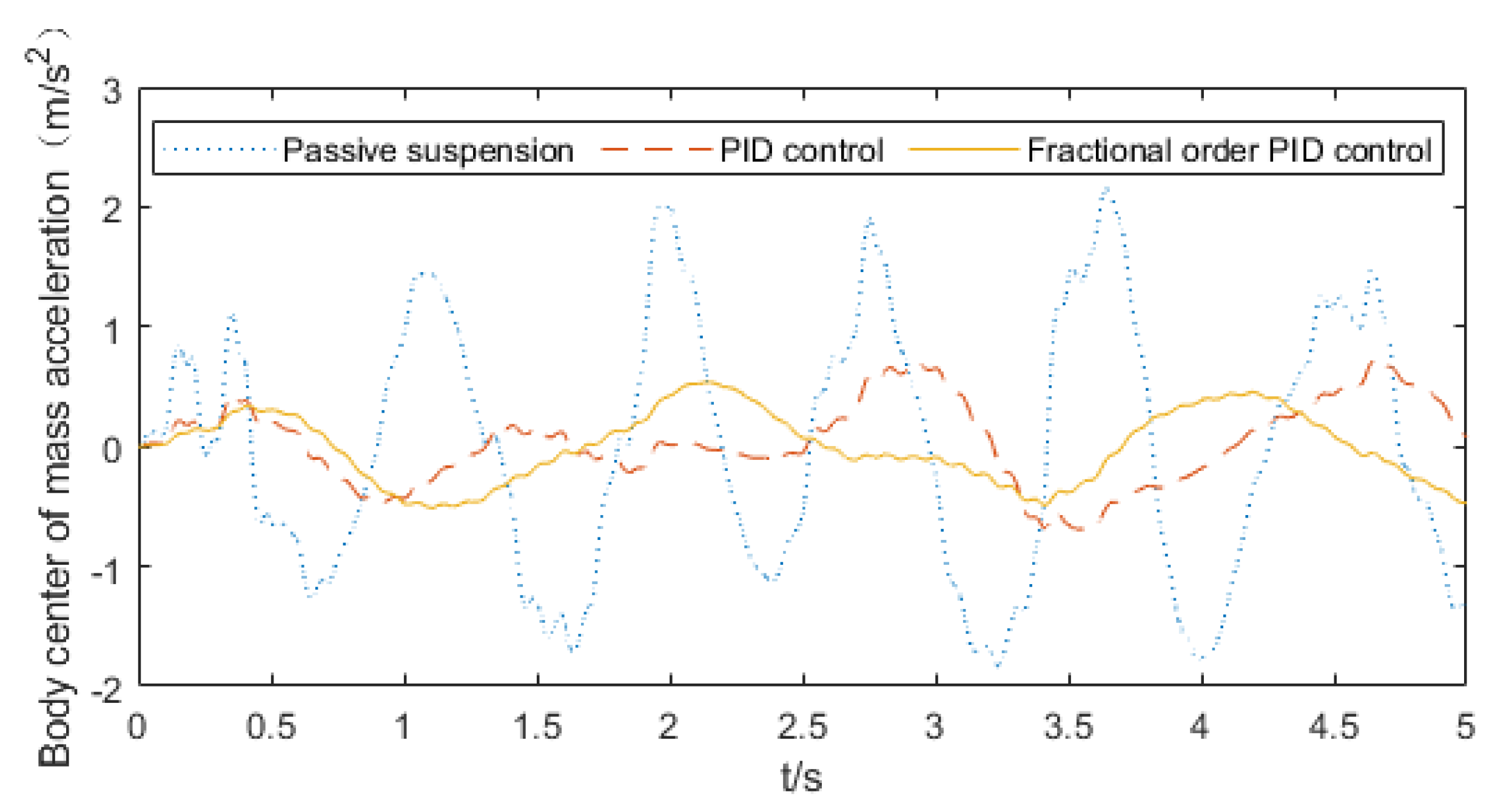
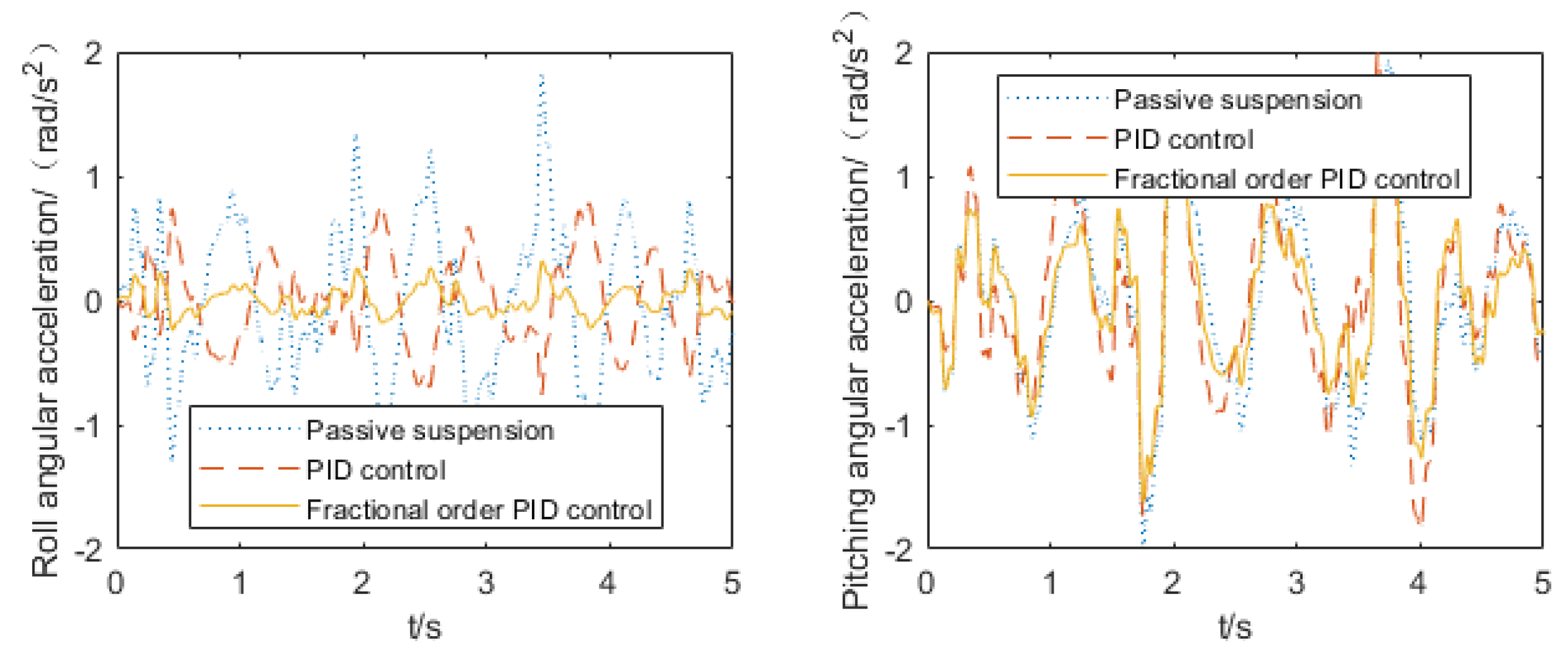
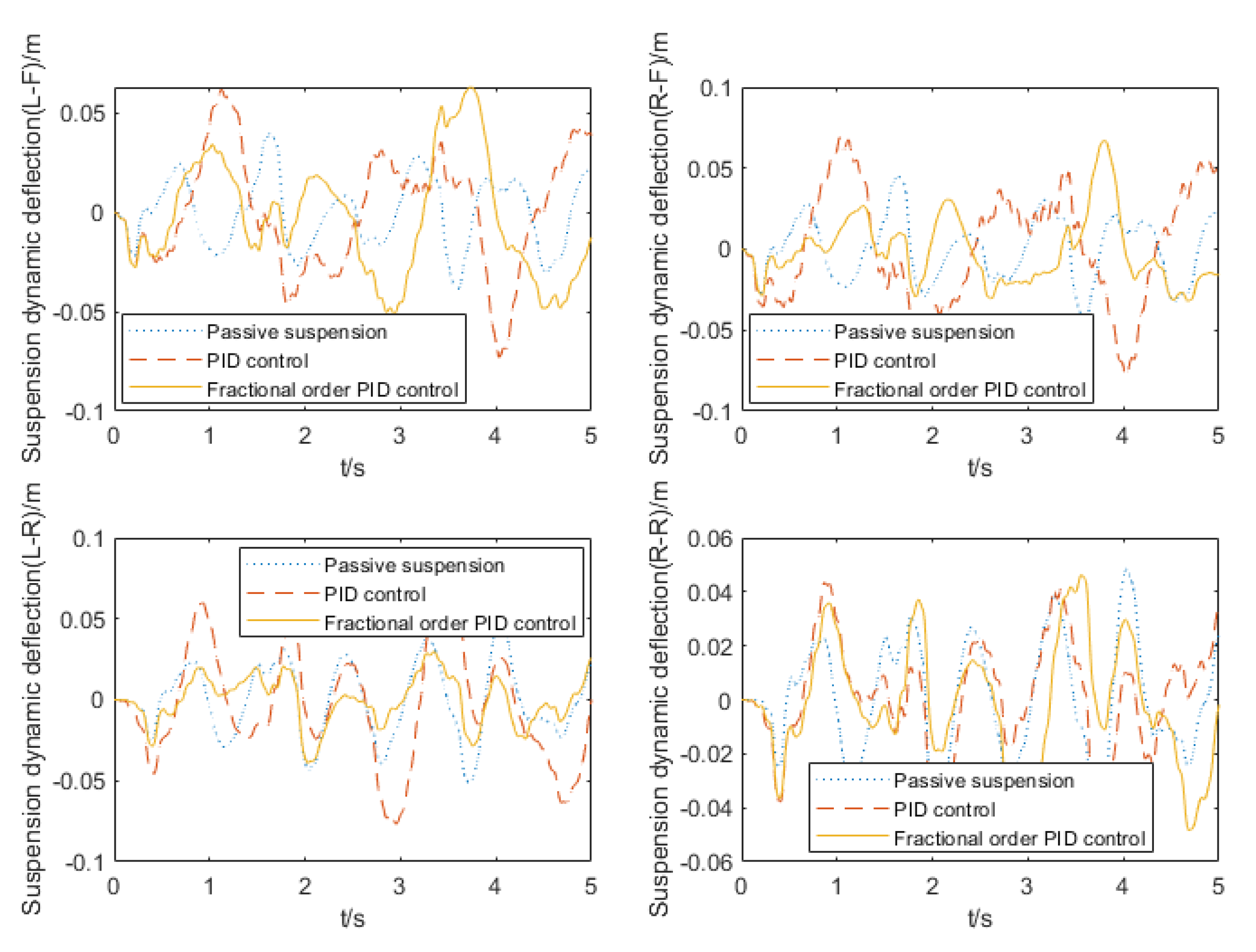
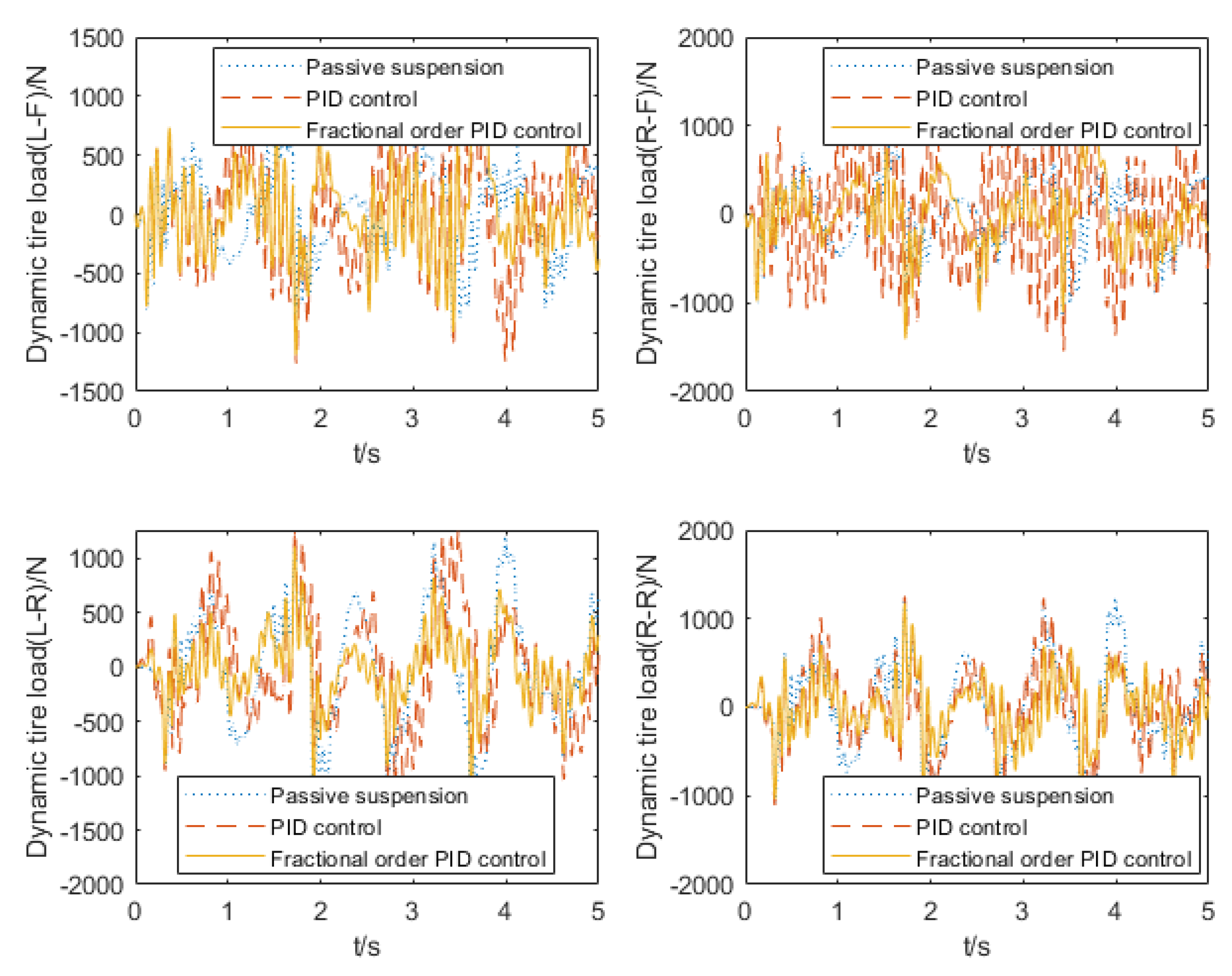
6.2. Simulation Analysis of Suspension System Vibration Damping Performance

The following Figure 16, Figure 17, Figure 18 and Figure 19 show the simulation images of each performance index under passive suspension, PID control, and fractional order PID control. In Figure 18 and Figure 19, L-F denotes the left front wheel, R-F denotes the right front wheel, L-R denotes the left rear wheel, and R-R denotes the right rear wheel.

Table 4. Table of root mean square values of performance index.

Performance Index	Control Method
	Passive Suspension	PID Control	FOPID Control
${\ddot{z}}_b/\mathrm{m}·{\mathrm{s}}^{-2}$	1.0531	0.3409	0.2791
$\ddot{\varphi }/\mathrm{rad}·{\mathrm{s}}^{-2}$	0.5820	0.3321	0.1066
$\ddot{\theta }/\mathrm{rad}·{\mathrm{s}}^{-2}$	0.7120	0.7120	0.5802
${(z}_{b_1}{-z}_1)/\mathrm{m}·{\mathrm{s}}^{-1}$	0.0178	0.0288	0.0282
${(z}_{b_2}{-z}_2)/\mathrm{m}·{\mathrm{s}}^{-1}$	0.0199	0.0342	0.0208
${(z}_{b_3}{-z}_3)/\mathrm{m}·{\mathrm{s}}^{-1}$	0.0221	0.0367	0.0148
${(z}_{b_4}{-z}_4)/\mathrm{m}·{\mathrm{s}}^{-1}$	0.0221	0.0231	0.0217
$k_1{(z}_1{-q}_1)$/N	374.6207	444.1296	353.8659
$k_2{(z}_2{-q}_2)/$N	427.0665	616.0492	390.4171
$k_3{(z}_3{-q}_3)/$N	562.2558	526.5663	351.9963
$k_4{(z}_4{-q}_4)/$N	576.0619	476.2702	376.7724

below shows the root mean square values of each index under various control methods.

From the data in Figure 16 and Figure 17 and Table 4, it can be seen that the PID control achieved optimization of body center of mass acceleration and roll angular acceleration compared to the passive suspension for four wheels with different road excitations, and fractional order PID control achieved optimization of body center of mass acceleration, roll angular acceleration and pitching angular acceleration. Under PID control, the center of mass acceleration was optimized to 32.37% of the passive suspension, the roll angular acceleration was optimized to 57.06% of the passive suspension, and the pitching angular acceleration was basically unchanged, compared to the passive suspension. The fractional order PID achieved a certain degree of optimization compared to the PID control. Its center of mass acceleration was optimized to 81.87% of the PID control, the roll angular acceleration was optimized to 32.10% of the PID control, and the pitching angular acceleration was optimized to 81.49% of the PID control. It can be seen that the active control of the whole vehicle studied in this paper, compared with the active control of the 1/4 suspension, not only achieved the optimization of the body acceleration, but also the optimization of the roll angular acceleration and the pitching angular acceleration, which makes a certain contribution to the improvement of the smoothness of the vehicle.

From the data in Figure 18 and Table 4, it can be seen that in order to make full use of the suspension dynamic deflection to achieve the optimization of driving smoothness, the suspension dynamic deflection under active control might increase to a certain extent compared with the passive suspension, and under PID control, the left front wheel suspension dynamic deflection increased to 161.80% of the passive suspension, the right front wheel increased to 171.86% of the passive suspension, the left rear wheel increased to 166.06% of the passive suspension, and the right rear wheel increased to 166.06%, and the right rear wheel increased to 104.52% of the passive suspension. The fractional order PID control suppressed the increase of the dynamic deflection of each wheel suspension to some extent, in which the left front wheel was suppressed to 97.92% of the PID control, the right front wheel was suppressed to 60.82% of the PID control, the left rear wheel was suppressed to 40.33% of the PID control, and the right rear wheel was suppressed to 93.94%.

From the data in Figure 19 and Table 4, it can be seen that the dynamic tire loads of the front suspension system deteriorated compared to the passive suspension under PID control, and the dynamic tire loads of the rear suspension system were all optimized to some extent. Among them, the left rear wheel was optimized to 93.65% of the passive suspension, and the right rear wheel was optimized to 82.68% of the passive suspension. Under the fractional order PID control, the dynamic tire loads of each suspension system were optimized to a stronger degree, compared to the passive suspension. Among them, the left front wheel was optimized to 94.46% of the passive suspension, the right front wheel was optimized to 91.42% of the passive suspension, the left rear wheel was optimized to 62.60% of the passive suspension, and the right rear wheel was optimized to 65.40% of the passive suspension.

In summary, fractional order PID control achieved greater optimization of body mass acceleration, roll angular acceleration, pitching angular acceleration and suspension dynamic load, compared to PID control, and also achieved the suppression of suspension dynamic deflection increase, which reflected the strong robustness of the fractional order PID controller in the face of the complex whole vehicle suspension system.

7. Conclusions

In this paper, the ball screw type energy regenerative active suspension system under fractional order PID control was studied, the mathematical model of each mechanism was established, and a series of studies were conducted through MATLAB 2018b and Simulink simulation and bench experiments. The contributions of the study are mainly as follows:

• The electromagnetic torque constant of the energy regenerative motor was obtained through the energy regenerative test and the calculation of the formula, which provides a method for measuring the electromagnetic torque constant of the energy regenerative motor.
• The digital implementation method of the fractional order PID control circuit for motor current was proposed, which provides a way for the practical application of fractional order PID control in engineering. The feasibility of the ball screw type energy regenerative actuator, and the superiority of the designed fractional order PID control circuit over the PID control circuit, were verified through simulation and test of the actuator control circuit.
• The objective function optimization results showed that the BAS algorithm can effectively optimize the parameters of the PID controller and the fractional order PID controller for active suspension control, and the speed and effect of the fractional order PID controller were better than those of the PID controller.
• The vehicle suspension system dynamics model was established, and the PID controller and the fractional order PID controller were used for active control of the vehicle. The control results showed that both the PID controller and the fractional order PID controller could optimize the driving smoothness to a certain extent, and the fractional order PID controller had a better optimization effect. Optimization of acceleration of pitching angle and acceleration of roll angle was a problem not involved in the 1/4 suspension active control. Under PID control, the front suspension system had a certain degree of deterioration of tire dynamic load, and the rear suspension system achieved a certain degree of optimization. Each tire dynamic load was optimized under fractional order PID control, due to the coupling of each performance index of the suspension, leading to active control of the fractional order PID controller, suppressing increase to a certain extent, and further demonstrating the superiority of the fractional order PID controller compared with the PID controller in dealing with complex control objects.

References

1. Fu, B.; Rocco, L.G.; Rickard, P.; Sebastian, S.; Stefano, B.; Roger, G. Active suspension in railway vehicles: A literature survey. Railw. Eng. Sci. 2020, 28, 3–35. [Google Scholar] [CrossRef] [Green Version]
2. Khalid, E.M.; Fouad, G.; Fatima-Zahra, C. Adaptive Backstepping Control Design for Semi-Active Suspension of Half-Vehicle with Magnetorheological Damper. IEEE/CAA J. Autom. Sin. 2021, 8, 582–596. [Google Scholar] [CrossRef]
3. Li, W.F.; Xie, Z.C.; Cao, Y.C.; Wong, P.K.; Zhao, J. Sampled-Data Asynchronous Fuzzy Output Feedback Control for Active Suspension Systems in Restricted Frequency Domain. IEEE/CAA J. Autom. Sin. 2021, 8, 1052–1066. [Google Scholar] [CrossRef]
4. Yashar, M.; Alireza, A.; Ibrahim, B.K.; Afef, F. Tube-based Model Reference Adaptive Control for Vibration Suppression of Active Suspension Systems. IEEE/CAA J. Autom. Sin. 2022, 9, 728–731. [Google Scholar] [CrossRef]
5. Chen, S.A.; Li, X.; Zhao, L.J. Development of a control method for an electromagnetic semi-active suspension reclaiming energy with varying charge voltage in steps. Int. J. Automot. Technol. 2015, 16, 765–773. [Google Scholar] [CrossRef]
6. Huang, K.; Yu, F.; Zhang, Y. Active controller design for an electromagnetic energy-regenerative suspension. Int. J. Automot. Technol. 2011, 12, 877–885. [Google Scholar] [CrossRef]
7. Amini, A.; Ekici, Ö.; Yakut, K. Experimental Study of Regenerative Rotational Damper in Low Frequencies. Int. J. Automot. Technol. 2020, 21, 83–90. [Google Scholar] [CrossRef]
8. Zhang, Y.; Chen, H.; Guo, K.; Zhang, X.; Li, S. Electro-hydraulic damper for energy harvesting suspension: Modeling, prototyping and experimental validation. Appl. Energy 2017, 199, 1–12. [Google Scholar] [CrossRef]
9. Zhu, S.; Shen, W.A.; Xu, Y.L. Linear electromagnetic devices for vibration damping and energy harvesting: Modeling and testing. Eng. Struct. 2012, 34, 198–212. [Google Scholar] [CrossRef] [Green Version]
10. Shin, S.S.; Kim, B.S.; Lee, D.W.; Kwon, S.J. Vehicle Dynamic Analysis for the Ball-Screw Type Energy Harvesting Damper System. Recent Adv. Electr. Eng. Relat. Sci. 2016, 415, 853–862. [Google Scholar] [CrossRef]
11. Narwade, P.; Deshmukh, R.; Nagarkar, M. Modeling and Simulation of a Semi-active Vehicle Suspension system using PID Controller. IOP Conf. Ser. Mater. Sci. Eng. 2020, 1004, 012003. [Google Scholar] [CrossRef]
12. Nagarkar, M.P.; Bhalerao, Y.J.; Vikhe Patil, G.J. GA-based multi-objective optimization of active nonlinear quarter car suspension system—PID and fuzzy logic control. Int. J. Mech. Mater. Eng. 2018, 13, 10. [Google Scholar] [CrossRef]
13. Wang, X.M. Microcontroller Control of Electric Motor, 4th ed.; Beijing University of Aeronautics and Astronautics Press: Beijing, China, 2015; pp. 84–85. [Google Scholar]
14. Podlubny, I. Fractional-order systems and PIλDμ-controllers. IEEE Trans Autom. Control 1999, 44, 208–214. [Google Scholar] [CrossRef]
15. Huang, Y.F. The Ball Screw Type Feeder Can Shock Absorber Design and Dynamics Analysis. Master’s Thesis, Shenyang University of Technology, Shenyang, China, 2017. Available online: https://kns.cnki.net/KCMS/detail/detail.aspx?dbname=CMFD201801&filename=1017094149.nh (accessed on 6 July 2022).
16. Jiang, X.; Li, S. BAS: Beetle Antennae Search Algorithm for Optimization Problems. Int. J. Robot. Control 2018, 1, 1–5. [Google Scholar] [CrossRef]
17. Zhang, Y.; Li, S.; Xu, B. Convergence analysis of beetle antennae search algorithm and its applications. Soft Comput. 2019, 25, 10595–10608. [Google Scholar] [CrossRef]
18. Huba, M.; Vrancic, D.; Bistak, P. PID Control With Higher Order Derivative Degrees for IPDT Plant Models. IEEE Access 2021, 9, 2478–2495. [Google Scholar] [CrossRef]
19. Yang, H.; Liu, J.; Li, M.; Zhang, X.; Liu, J.; Zhao, Y. Adaptive Kalman Filter with L2 Feedback Control for Active Suspension Using a Novel 9-DOF Semi-Vehicle Model. Actuators 2021, 10, 267. [Google Scholar] [CrossRef]
20. Pakdelian, S. A compact and light-weight generator for backpack energy harvesting. In Proceedings of the 2016 IEEE Energy Conversion Congress and Exposition (ECCE), Milwaukee, WI, USA, 18–22 September 2016; Volume 1, pp. 1–8. [Google Scholar] [CrossRef]
21. Li, Z.C. Structural Selection and Performance Simulation of Automotive Energy-Feeding Suspension. Master’s Thesis, Jilin University, Jilin, China, 2009. Available online: https://kns.cnki.net/KCMS/detail/detail.aspx?dbname=CMFD2009&filename=2009094256.nh (accessed on 6 July 2022).
22. Ahamed, R.; Rashid, M.M.; Ferdaus, M.M. Design and modeling of energy generated magneto rheological damper. Korea-Aust. Rheol. J. 2016, 28, 67–74. [Google Scholar] [CrossRef]
23. Liu, Q.Y. Research on Energy-Feeding Suspension Control Algorithm. Master’s Thesis, Jilin University, Jilin, China, 2019. Available online: https://kns.cnki.net/KCMS/detail/detail.aspx?dbname=CMFD201902&filename=1019155509.nh (accessed on 6 July 2022).
24. Kou, F.R. Theory and Technology of Active Control of Automotive Vibration, 1st ed.; Huazhong University of Science and Technology Press: Wuhan, China, 2021; pp. 100–114. [Google Scholar]
25. Kril, S.; Fedoryshyn, R.; Kril, O.; Pistun, Y. Investigation of Functional Diagrams of Step PID Controllers for Electric Actuators. Procedia Eng. 2015, 100, 1338–1347. [Google Scholar] [CrossRef] [Green Version]
26. Li, X.J.; Liu, J.; Liu, Z.H. Research on BP Neural Network PID Control of Energy Regenerative Suspension. Mod. Manuf. Eng. 2020, 3, 60–65+135. [Google Scholar] [CrossRef]
27. Pritesh, S.; Sudhir, A. Review of fractional PID controller. Mechatronics 2016, 38, 29–41. [Google Scholar] [CrossRef]
28. Axtell, M.; Bise, M.E. Fractional calculus application in control systems. In Proceedings of the IEEE Conference on Aerospace and Electronics, Dayton, OH, USA, 21–25 May 1990; Volume 2, pp. 563–566. [Google Scholar] [CrossRef]
29. Hamamci, S.E. Stabilization using fractional-order PI and PID controllers. Nonlinear Dyn. 2008, 51, 329–343. [Google Scholar] [CrossRef]
30. Xue, D.Y.; Zhao, C.N.; Chen, Y.Q. A Modified Approximation Method of Fractional Order System. In Proceedings of the IEEE Conference on Mechatronics and Automation, Luoyang, China, 25–28 June 2006; pp. 1043–1048. [Google Scholar]
31. Fan, Y.Q.; Shao, J.P.; Sun, G.T. Optimized PID Controller Based on Beetle Antennae Search Algorithm for Electro-Hydraulic Position Servo Control System. Sensors 2019, 19, 2727. [Google Scholar] [CrossRef] [PubMed] [Green Version]
Figure 1. Selection range of different types of PID controllers.
Actuators 11 00189 g001
Figure 2. Structure of the 1/4 energy regenerative active suspension.
Actuators 11 00189 g002
Figure 3. Model of the complete vehicle suspension system.
Actuators 11 00189 g003
Figure 4. Structure of the 1/4 energy regenerative active suspension.
Actuators 11 00189 g004
Figure 5. Motor four-quadrant operation diagram.
Actuators 11 00189 g005
Figure 6. Equivalent circuit diagram of the energy regenerative motor.
Actuators 11 00189 g006
Figure 7. Equivalent circuit diagram of the energy regenerative motor.
Actuators 11 00189 g007
Figure 8. Equipment for energy recovery tests. (a) General assembly drawing of the test stand and workflow; (b) Diagram of the energy recovery actuator.
Actuators 11 00189 g008
Figure 9. Instantaneous energy recovery power at different frequencies.
Actuators 11 00189 g009
Figure 10. Control circuit test bench and test procedure.
Actuators 11 00189 g010
Figure 11. Results of current control experiment.
Actuators 11 00189 g011
Figure 12. Block diagram of the suspension system control principle.
Actuators 11 00189 g012
Figure 13. Optimization flow chart of Beetle Antennae Search Algorithm.
Actuators 11 00189 g013
Figure 14. Objective function optimization curve.
Actuators 11 00189 g014
Figure 15. Comparison of the control force of each actuator.
Actuators 11 00189 g015
Figure 16. Simulation image of body center of mass acceleration.
Actuators 11 00189 g016
Figure 17. Pitching angular acceleration and roll angular acceleration simulation results.
Actuators 11 00189 g017
Figure 18. Suspension dynamic deflection simulation results.
Actuators 11 00189 g018
Figure 19. Dynamic tire load simulation results.
Actuators 11 00189 g019