A Novel High-Speed Third-Order Sliding Mode Observer for Fault-Tolerant Control Problem of Robot Manipulators

Abstract

In this paper, a novel fault-tolerant control tactic for robot manipulator systems using only position measurements is proposed. The proposed algorithm is constructed based on a combination of a nonsingular fast terminal sliding mode control (NFTSMC) and a novel high-speed third-order sliding mode observer (TOSMO). In the first step, the high-speed TOSMO is proposed for the first time to approximate both the system velocity and the lumped unknown input with a faster convergence time compared to the TOSMO. The faster convergence speed is obtained thanks to the linear characteristic of the added elements. In the second step, the NFTSMC is designed based on a nonsingular fast terminal sliding (NFTS) surface and the information obtained from the proposed high-speed TOSMO. Thanks to the combination, the proposed controller–observer tactic provides excellent features, such as a fast convergence time, high tracking precision, chattering phenomenon reduction, robustness against the effects of the lumped unknown input and velocity requirement elimination. Especially, the proposed observer does not only improve the convergence speed of the estimated signals, but also increases the system dynamic response. The system’s finite-time stability is proved using the Lyapunov theory. Finally, to validate the efficiency of the proposed strategy, simulations on a PUMA560 robot manipulator are performed.

1. Introduction

In the industry, robot manipulators are employed widely in various applications, such as material handling, milling, painting, welding and roughing. Along with the growth of robot manipulator applications, interest in robotic control has been increased [1,2,3,4]. In some research, the robot’s end-effector position is required to track the desired trajectory. For this purpose, the kinematics control approach is preferred [5,6]. Another approach is to use the dynamics control when joint angles are preferred [7,8]. Generally, robot manipulators are difficult to control in both theoretical and practical aspects due to some of their characteristics. First, robot manipulator systems have a highly nonlinear and very complex dynamic in coupling terms. Additionally, payload changes, friction, external disturbances, etc., lead to robot dynamic uncertainty. Therefore, obtaining the robot’s correct dynamics is arduous or even impossible. In some special cases, in long-term operation, unknown faults can occur when the robot is operating, which includes actuator faults or sensor faults. Further, to reduce the weight/size and save costs, in some cases, manufacturers remove the velocity sensors in the robot. These are big problems that have been challenged by many researchers. To simplify the presentation and avoid duplication, in this article, the dynamic uncertainty and the unknown fault are treated and abbreviated as a lumped unknown input.

To deal with the aforementioned lumped unknown input, many control methods have been developed, such as proportional–integral–derivative (PID) control [9,10], adaptive control [11], fuzzy control [12], neural network (NN) control [13] and sliding mode control (SMC) [14,15]. PID control is well-known as a simple and monotonic controller, which does not require the dynamic model of the robot system. However, this controller cannot achieve high tracking performance. Adaptive control is an effective method to deal with matched uncertainties; however, it is not appropriate for the problem of mismatched uncertainties. Intelligent control schemes are widely employed, such as NN control and fuzzy control. The learning ability and good approximation of nonlinear function with the arbitrary accuracy of NN controllers make them a good choice for modelling complex processes and compensating for mismatched uncertainties. However, transient performance in the presence of a disturbance can be degraded due to the required online learning procedure. The fuzzy logic control method was developed based on expert knowledge and experience; however, its main disadvantages are difficulties in the stability analysis and comprehensive knowledge of the requirements of a system. SMC is one of the most powerful robust controllers that has been widely utilized in the fault-tolerant control problem of robot manipulators due to its effectiveness in rejecting the effects of the lumped unknown input [16,17,18]. Moreover, the design procedure of SMC is not complex and quite popular in the literature [19,20,21]. Unfortunately, conventional SMC uses a linear sliding surface that means the finite-time convergence cannot be guaranteed. In order to achieve a finite-time convergence, a nonlinear sliding surface is utilized instead of a linear one in the design process of the controller; this technique is well-known as terminal SMC (TSMC) [22,23]. Compared to conventional SMC, TSMC extends two outstanding properties, which are finite-time convergence and achieving higher accuracy when parameters are carefully designed. Unfortunately, TSMC only obtains a faster convergence when system states are near the equilibrium point, but slower when the system states are far from the equilibrium point. In addition, TSMC suffers from the singularity problem. The two problems have been handled separately using fast TSMC (FTSMC) [24,25] and nonsingular TSMC (NTSMC) [26,27,28]. In order to solve both problems at the same time, nonsingular fast TSMC (NFTSMC) was developed [29,30,31]. Due to its excellent control features, such as providing finite-time convergence, eliminating the singularity problem, achieving high-position tracking precision and robustness against the lumped unknown input, NFTSMC has been applied widely in the literature. However, same as SMC and TSMC, utilizing a discontinuous switching element with a big and fixed sliding gain to handle the effects of the lumped unknown input in the designing process of NFTSMC is the root of high-frequency oscillations, the so-called chattering [32]. This phenomenon harms the system; therefore, it decreases the practical applicability of SMC. In addition, the design procedure of NFTSMC involves real velocity information, which is sometimes unavailable in practical systems.

To resolve the chattering problem, the elementary idea is to reduce the sliding gain in the switching control component. In this approach, the lumped unknown input is first completely or partially estimated. After that, the estimated unknown input is applied in a controller design as a compensator to reduce the lumped unknown input effects. Therefore, the switching control component is now utilized to carry out the impacts of the estimation error instead of the lumped unknown input as in the original controller. As a result, the sliding gain is chosen with a smaller value, thus, the chattering phenomenon can be reduced. In the literature, various techniques for fault diagnosis have been proposed to approximate the lumped unknown input, such as the NN observer [33,34], adaptive observer [35,36], time-delay estimation [37,38], linear extended state observer (LESO) [39,40], second-order sliding mode observer (SOSMO) [41] and third-order sliding mode observer (TOSMO) [42,43]. Among them, the SOSMO and the TOSMO stand out with the capability to estimate not only the lumped unknown input, but also the velocity information; therefore, the requirement of the tachometer is eliminated without the need of an additional state observer. Concerning the comparison of the above two observers, the main advantage of the SOSMO is its ability to provide a faster approximation speed. In contrast, the TOSMO can provide estimation signals with a higher estimation accuracy and less chattering, without any filtration. Unfortunately, as a trade-off, its convergence speed becomes slower than that of the SOSMO. Therefore, it is necessary to design an observer that can combine the wonderful properties of both the SOSMO and the TOSMO.

Motivated by all the above discussions, this paper first proposes a novel high-speed TOSMO for the robot manipulator system by adding additional terms to the original TOSMO. This observer can not only maintain the remarkable benefits of the original TOSMO, but also obtain a faster convergence time. The estimated velocity and unknown input are then applied to design a fault-tolerant control based on NFTSMC. The major contributions of this paper are summarized as follows:

• The proposal of a novel high-speed TOSMO that can obtain a faster convergence speed while maintaining the high estimation accuracy of the TOSMO;
• The proposal of a fault-tolerant control law based on NFTSMC and the proposed high-speed TOSMO that handles the effects of the lumped unknown input to achieve a higher tracking accuracy and low chattering phenomenon;
• The provision of proof of the system finite-time stability when combining a controller and observer.

This paper is organized into six parts. Following the introduction, the mathematical dynamics model of robot manipulators and problem formulation are presented in Section 2. In Section 3, the design of the high-speed TOSMO is presented, followed by the design procedure of the fault-tolerant control law based on NFTSMC for the robot manipulators shown in Section 4. To confirm the efficiency of the proposed method, computer simulations on a PUMA560 robot manipulator are shown in Section 5. Finally, Section 6 gives some conclusions.

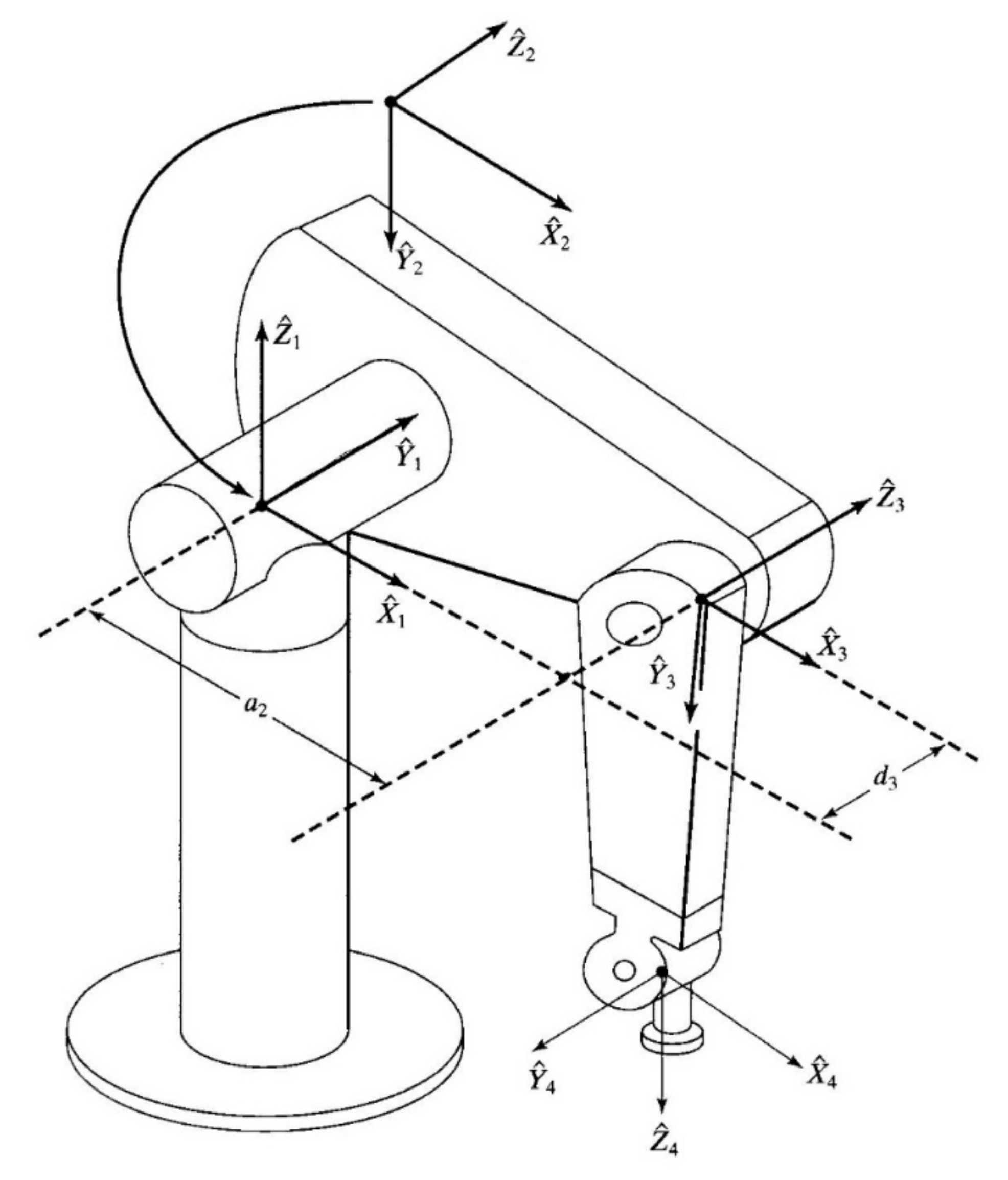
2. Mathematical Dynamics Model of Robot Manipulators and Problem Formulation

2.1. Robot Dynamics

Let us consider a serial n-link robot manipulator under the effects of dynamic uncertainty and unknown fault as follows:

$$\ddot{q}=M{\left(q\right)}^{-1}\left[\tau \left(t\right)-C\left(q,\dot{q}\right)\dot{q}-G\left(q\right)-F_r\left(\dot{q}\right)-{\tau }_d\left(t\right)\right] +\mathrm{\Omega }\left(q,\dot{q},t\right)$$

(1)

where $q,\dot{q},\ddot{q}\in {\Re }^n$ correspondingly represent the robot’s joint positions, velocity and acceleration vectors; $M\left(q\right)\in {\Re }^{n\times n}$ represents the inertia matrix, which is symmetric and positively definite, making it invertible; $C\left(q,\dot{q}\right)\in {\Re }^{n\times n}$, $G\left(q\right)\in {\Re }^n$ and $F_r\left(\dot{q}\right)\in {\Re }^n$ denote the Coriolis and centripetal forces, gravitational vector and friction vector, respectively; ${\tau }_d(t)\in {\Re }^n$ denotes the disturbance vector; $\tau (t)\in {\Re }^n$ denotes the control input signal; and $\mathrm{\Omega }\left(q,\dot{q},t\right)=\omega \left(t-T_f\right)\mathrm{\Phi }\left(q,\dot{q}\right)$ denotes the unknown but bounded fault with the time profile $\omega \left(t-T_f\right)=diag\left\{{\omega }_1\left(t-T_f\right),{\omega }_2\left(t-T_f\right),\dots ,{\omega }_n\left(t-T_f\right)\right\}$, where ${\omega }_i\left(t-T_f\right)=\left\{\begin{array}{c}0 if t\le T_f\\ 1-e^{-{\zeta }_i\left(t-T_f\right)} if t\ge T_f\end{array}\right.$. The unknown fault function $\mathrm{\Phi }\left(q,\dot{q}\right)$ occurs at time $T_f$ with evolution rate ${\zeta }_i>0 , \left(i=1,2,\dots ,n\right)$.

By defining $u=\tau (t)$ and $x={\left[\begin{array}{cc}{x}_1{}^T& x_2{}^T\end{array}\right]}^T$ with $x_1=q$, $x_2=\dot{q}$, we could transfer system (1) into the state space form as

$$\begin{array}{l}{\dot{x}}_1=x_2\\ {\dot{x}}_2=\mathrm{\Psi }(x)+M{\left(x_1\right)}^{-1}u+\mathrm{\Delta }(x,t)\end{array}$$

(2)

where $\mathrm{\Psi }(x)=M{\left(q\right)}^{-1}\left[-C\left(q,\dot{q}\right)-G\left(q\right)\right]$ represents the nominal model of robot manipulators and $\mathrm{\Delta }(x,t)=M{\left(q\right)}^{-1}\left[-F_r\left(\dot{q}\right)-{\tau }_d\right]+\mathrm{\Omega }\left(q,\dot{q},t\right)$ denotes the lumped unknown but bounded dynamic uncertainty and unknown fault.

Remark 1.

In this paper, the unknown fault was considered as an additional dynamic uncertainty; therefore, their total effects on the system were carried out. We simply named them the lumped unknown input.

2.2. Problem Formulation

Let $x_d\in {\Re }^n$ be an expected trajectory of a robot’s joint, where the tracking error is defined as

$$e=x_1-x_d$$

(3)

The central purpose of this paper was divided into two parts. First, a novel high-speed TOSMO was proposed for the first time to estimate both a system’s states and the lumped unknown input with high precision and a fast response time. Second, based on the achieved information from the proposed observer, a fault-tolerant control approach using NFTSMC was then designed for system (2) to ensure that the joint position $x_1$ could track the desired trajectory $x_d$ with high accuracy, even in the presence of the lumped unknown input and the absence of the velocity measurement. In addition, the controller further demonstrated the effectiveness of the proposed high-speed TOSMO. The proposed algorithm was constructed based on assumptions as follows:

Assumption 1.

The desired trajectory $x_d$was a twice continuously differentiable function in respect to time $t$.

Assumption 2.

The lumped unknown input $\mathrm{\Delta }(x,t)$was bounded by a positive constant ${\mathrm{\Delta }}_D$as

$$\left|\mathrm{\Delta }(x,t)\right|\le {\mathrm{\Delta }}_D$$

(4)

Assumption 3.

The derivative of the lumped unknown input $\mathrm{\Delta }(x,t)$in respect to time existed and was bounded by a positive constant ${\mathrm{\Delta }}_{\dot{D}}$as

$$\left|\frac{d}{dt}\mathrm{\Delta }(x,t)\right|\le {\mathrm{\Delta }}_{\dot{D}}$$

(5)

Note that Assumption 3 is realistic and has been used in much research [44,45,46].

3. Design of Observer

3.1. High-Speed Third-Order Sliding Mode Observer

In this section, a novel high-speed TOSMO was proposed by adding additional terms to the original TOSMO. Thanks to the linear characteristic of these terms, which can strongly deal with perturbations that are very far away from the origin, the slow convergence problem of the TOSMO was improved.

Based on system (2), the novel high-speed TOSMO was proposed as follows:

$$\begin{array}{l}{\dot{\widehat{x}}}_1=k_1{\left|x_1-{\widehat{x}}_1\right|}^{2/3}sign\left(x_1-{\widehat{x}}_1\right)+{\widehat{x}}_2+\mathit{\Gamma }\left(x_1-{\widehat{x}}_1\right)\\ {\dot{\widehat{x}}}_2=\mathrm{\Psi }(\widehat{x})+M{\left(x_1\right)}^{-1}u+k_2{\left|x_1-{\widehat{x}}_1\right|}^{1/3}sign\left(x_1-{\widehat{x}}_1\right)+\Gamma \left({\dot{\widehat{x}}}_1-{\widehat{x}}_2\right)-\widehat{z}\\ \dot{\widehat{z}}=-k_{3}sign\left(x_1-{\widehat{x}}_1\right)\end{array}$$

(6)

where $\widehat{x}$ is the estimation of $x$, $k_i$$\left(i=1, 2, 3\right)$ denotes the sliding gains and $\mathrm{\Gamma }$ is a positive constant. In the proposed observer, the additional terms were bolded to distinguish them from the original TOSMO.

Theorem 1.

For the robot manipulator system given in (2) with the high-speed TOSMO (6), if the sliding gains of the observer were chosen as Remark 3, then the proposed observer was stable and the estimation states $\left({\widehat{x}}_1, {\widehat{x}}_2\right)$would achieve the real states$\left(x_1, x_2\right)$in finite time.

Proof of Theorem 1.

By subtracting (6) from (2), we obtained the estimation errors as

$$\begin{array}{l}{\dot{\tilde{x}}}_1=-k_1{\left|{\tilde{x}}_1\right|}^{2/3}sign\left({\tilde{x}}_1\right)+{\tilde{x}}_2-\mathrm{\Gamma }{\tilde{x}}_1\\ {\dot{\tilde{x}}}_2=-k_2{\left|{\tilde{x}}_1\right|}^{1/3}sign\left({\tilde{x}}_1\right)-\mathrm{\Gamma }\left({\dot{\widehat{x}}}_1-{\widehat{x}}_2\right)+\mathrm{\Delta }(x,t)-\delta (x,\tilde{x})+\widehat{z}\\ \dot{\widehat{z}}=-k_{3}sign\left({\tilde{x}}_1\right)\end{array}$$

(7)

where ${\tilde{x}}_1=x_1-{\widehat{x}}_1$ and ${\tilde{x}}_2=x_2-{\widehat{x}}_2$ represent the position and velocity estimation errors, respectively. The estimation error $\delta (x,\tilde{x})=\mathrm{\Psi }(\widehat{x})-\mathrm{\Psi }(x)$. To facilitate the next design approach, in this phase, we assumed that $\left|\delta (x,\tilde{x})\right|\le {\mathrm{\Delta }}_{\delta }$ and $\left|\dot{\delta }(x,\tilde{x})\right|\le {\mathrm{\Delta }}_{\dot{\delta }}$, where ${\mathrm{\Delta }}_{\delta }$ and ${\mathrm{\Delta }}_{\dot{\delta }}$, were positive constants. Note that this assumption was the same as Assumption 3; thus, it could be supported in both theoretical and practical applications.

Substituting the first term of (6) into (7), we obtained

$$\begin{array}{l}{\dot{\tilde{x}}}_1=-k_1{\left|{\tilde{x}}_1\right|}^{2/3}sign\left({\tilde{x}}_1\right)+{\tilde{x}}_2-\mathrm{\Gamma }{\tilde{x}}_1\\ {\dot{\tilde{x}}}_2=-k_2{\left|{\tilde{x}}_1\right|}^{1/3}sign\left({\tilde{x}}_1\right)+\mathrm{\Delta }(x,t)-\delta (x,\tilde{x})+\widehat{z}-\mathrm{\Gamma }{k}_1{\left|{\tilde{x}}_1\right|}^{2/3}sign\left({\tilde{x}}_1\right)-{\mathrm{\Gamma }}^2{\tilde{x}}_1\\ \dot{\widehat{z}}=-k_{3}sign\left({\tilde{x}}_1\right)\end{array}$$

(8)

By defining the new variable $\overline{x}={\tilde{x}}_2-\mathrm{\Gamma }{\tilde{x}}_1$, the estimation errors in (8) were rewritten as

$$\begin{array}{l}{\dot{\tilde{x}}}_1=-k_1{\left|{\tilde{x}}_1\right|}^{2/3}sign\left({\tilde{x}}_1\right)+\overline{x}\\ \dot{\overline{x}}=-k_2{\left|{\tilde{x}}_1\right|}^{1/3}sign\left({\tilde{x}}_1\right)+\mathrm{\Delta }(x,t)-\delta (x,\tilde{x})+\widehat{z}\\ -\mathrm{\Gamma }{k}_1{\left|{\tilde{x}}_1\right|}^{2/3}sign\left({\tilde{x}}_1\right)-{\mathrm{\Gamma }}^2{\tilde{x}}_1\\ \underset{-\mathrm{\Gamma }{\dot{\tilde{x}}}_1}{\underbrace{+\mathrm{\Gamma }{k}_1{\left|{\tilde{x}}_1\right|}^{2/3}sign\left({\tilde{x}}_1\right)+{\mathrm{\Gamma }}^2{\tilde{x}}_1-\mathrm{\Gamma }{\tilde{x}}_2}}\\ \dot{\widehat{z}}=-k_{3}sign\left({\tilde{x}}_1\right)\end{array}$$

(9)

Letting $\widehat{\mathrm{\Delta }}(x,t)=\mathrm{\Delta }(x,t)-\delta (x,\tilde{x})+L$, the system (9) became

$$\begin{array}{l}{\dot{\tilde{x}}}_1=-k_1{\left|{\tilde{x}}_1\right|}^{2/3}sign\left({\tilde{x}}_1\right)+\overline{x}\\ \dot{\overline{x}}=-k_2{\left|{\tilde{x}}_1\right|}^{1/3}sign\left({\tilde{x}}_1\right)+\widehat{\mathrm{\Delta }}(x,t)+\widehat{z}\\ \dot{\widehat{z}}=-k_{3}sign\left({\tilde{x}}_1\right)\end{array}$$

(10)

where $L=-\mathrm{\Gamma }{\tilde{x}}_2$ with the assumptions were that $\left|L\right|\le {\mathrm{\Delta }}_L$ and $\left|\frac{d}{dt}L\right|\le {\mathrm{\Delta }}_{\dot{L}}$.

By defining ${\tilde{x}}_3=\widehat{z}+\widehat{\mathrm{\Delta }}(x,t)$, the system in (10) could be rewritten in the same form of the second-order sliding mode differentiator [47] as

$$\begin{array}{l}{\dot{\tilde{x}}}_1=-k_1{\left|{\tilde{x}}_1\right|}^{2/3}sign\left({\tilde{x}}_1\right)+\overline{x}\\ \dot{\overline{x}}=-k_2{\left|{\tilde{x}}_1\right|}^{1/3}sign\left({\tilde{x}}_1\right)+{\tilde{x}}_3\\ {\dot{\tilde{x}}}_3=-k_{3}sign\left({\tilde{x}}_1\right)+\dot{\widehat{\mathrm{\Delta }}}(x,t)\end{array}$$

(11)

Equation (11) is also as well-known as the TOSMO [48]. By selecting the candidate Lyapunov function $V_0$ and using the same demonstrating process as in [48], it could be concluded that system (11) was stable and the differentiators ${\tilde{x}}_1,$$\overline{x}$ and ${\tilde{x}}_3$ converged to zero in finite time. Thus, system (7) was stable and the estimation errors ${\tilde{x}}_1,$${\tilde{x}}_2$ converged to zero in finite time. □

Remark 2.

The proposed high-speed TOSMO in (6) was designed based on the original TOSMO in [42]. The linear characteristics of the added terms were utilized to increase the convergence speed of the estimated signals.

Remark 3.

The observer gains of (6) were selected according to [47] as $k_1={\alpha }_1{\overline{\mathrm{\Delta }}}^{1/3}$, $k_2={\alpha }_2{\overline{\mathrm{\Delta }}}^{2/3}$ and $k_3={\alpha }_3\overline{\mathrm{\Delta }}$, where ${\alpha }_1=2$, ${\alpha }_2=2.12$ and ${\alpha }_3=1.1$ with $\overline{\mathrm{\Delta }}={\mathrm{\Delta }}_{\dot{D}}+{\mathrm{\Delta }}_{\dot{\delta }}+{\mathrm{\Delta }}_{\dot{L}}$.

3.2. Unknown Input Identification

After the convergence time, the estimated velocity reached the real velocity, ${\widehat{x}}_2=x_2$; thus, the term $L=-\mathrm{\Gamma }{\tilde{x}}_2$ converged to zero. The third term of system (11) then became

$${\dot{\tilde{x}}}_3=-k_{3}sign\left({\tilde{x}}_1\right)+\dot{\widehat{\mathrm{\Delta }}}(x,t)\equiv 0$$

(12)

Notably, because the velocity estimation error ${\tilde{x}}_2$ converged to zero, the auxiliary unknown input term $\widehat{\mathrm{\Delta }}(x,t)=\mathrm{\Delta }(x,t)-\delta (x,\tilde{x})+L$ converged to $\mathrm{\Delta }(x,t)$.

The lumped unknown input terms could be rebuilt as

$$\widehat{\mathrm{\Delta }}(x,t)={\displaystyle \mathrm{\int }{k}_{3}sign\left({\tilde{x}}_1\right)}$$

(13)

Since the estimated unknown input in (13) included an integral operation, the lumped unknown input terms could be rebuilt directly from the output injection term, and the chattering of the obtained function was partially eliminated without the need for a lowpass filter. In addition, the proposed observer in (6) not only maintained the advantages of the conventional TOSMO such as the finite-time convergence and high estimation accuracy for both velocity and the lumped unknown input, but also provided a faster convergence time than that of the TOSMO. The outstanding features of the proposed high-speed TOSMO were verified in the simulation part.

Remark 4.

The obtained lumped unknown input could be used for fault detection and fault isolation and could also be applied to the fault-tolerant control to eliminate its effect on the system. The estimated velocity could be employed in the controller design process instead of the real measured velocity.

4. Design of Control Algorithm

In this section, a fault-tolerant control tactic using the NFTSMC algorithm was proposed to carry out the effects of the lumped unknown input of system (2). In addition, in some special cases, the tachometers in robots would be cut off by manufacturers to save cost and reduce weight. For that reason, this paper assumed that the tachometers did not exist. The estimated velocity, ${\widehat{x}}_2$, which was obtained from the proposed observer in Section 3, was utilized; therefore, the requirement of the real measured velocity was eliminated.

4.1. Design of Nonsingular Fast Terminal Sliding Surface

Let us define the estimated velocity error as

$$\widehat{\dot{e}}={\widehat{x}}_2-{\dot{x}}_d$$

(14)

where ${\dot{x}}_d$ describes the desired velocity.

A NFTS surface was selected as in [49]

$$\widehat{s}=\widehat{\dot{e}}+{\displaystyle \mathrm{\int }\left[{\beta }_1{\left|e\right|}^{{\gamma }_1}sign\left(e\right)+{\beta }_2{\left|\widehat{\dot{e}}\right|}^{{\gamma }_2}sign\left(\widehat{\dot{e}}\right)+{\beta }_{3}e+{\beta }_4{e}^3\right]}dt$$

(15)

where the parameters ${\beta }_1, {\beta }_2, {\beta }_3, {\beta }_4$ are positive constants and the parameters ${\gamma }_1, {\gamma }_2$ could be selected as $0<{\gamma }_1<1, {\gamma }_2=2{\gamma }_1/(1+{\gamma }_1)$.

According to the SMC theory, the following conditions were satisfied when the robot system reached the sliding mode:

$$\begin{array}{l}\widehat{s}=0\\ \dot{\widehat{s}}=0\end{array}$$

(16)

Thus, the sliding mode dynamics could be acquired as

$$\widehat{\dot{e}}=-{\displaystyle \mathrm{\int }\left[{\beta }_1{\left|e\right|}^{{\gamma }_1}sign\left(e\right)+{\beta }_2{\left|\widehat{\dot{e}}\right|}^{{\gamma }_2}sign\left(\widehat{\dot{e}}\right)+{\beta }_{3}e+{\beta }_4{e}^3\right]}dt$$

(17)

Theorem 2.

For the sliding mode dynamics in (17), the origin was defined as the stable equilibrium point and the state trajectories converged to zero in finite time.

Proof of Theorem 2.

Taking the derivative of the tracking error in (3) in respect to time yielded

$$\begin{array}{l}\dot{e}={\dot{x}}_1-{\dot{x}}_d\\ =x_2-{\dot{x}}_d\end{array}$$

(18)

Based on the definition of the estimation errors in Section 3, the velocity error (14) was rewritten as

$$\begin{array}{l}\widehat{\dot{e}}={\widehat{x}}_2-{\dot{x}}_d\\ =x_2-{\dot{x}}_d-{\tilde{x}}_2\end{array}$$

(19)

After the convergence time of the estimation errors (7), the estimated velocity, ${\widehat{x}}_2$, reached the true velocity, $x_2$. Hence, the velocity error (19) became

$$\widehat{\dot{e}}=x_2-{\dot{x}}_d=\dot{e}$$

(20)

The sliding mode dynamics in (17) became

$$\dot{e}=-{\displaystyle \mathrm{\int }\left[{\beta }_1{\left|e\right|}^{{\gamma }_1}sign\left(e\right)+{\beta }_2{\left|\dot{e}\right|}^{{\gamma }_2}sign\left(\dot{e}\right)+{\beta }_{3}e+{\beta }_4{e}^3\right]}dt$$

(21)

Then, the following sliding mode dynamics could be obtained

$$\ddot{e}=-{\beta }_1{\left|e\right|}^{{\gamma }_1}sign\left(e\right)-{\beta }_2{\left|\dot{e}\right|}^{{\gamma }_2}sign\left(\dot{e}\right)-{\beta }_{3}e-{\beta }_4{e}^3$$

(22)

A Lyapunov function candidate was selected as

$$V_1=\frac{{\beta }_1}{{\gamma }_1+1}{\left|e\right|}^{{\gamma }_1+1}+\frac{1}{2}{\dot{e}}^2+\frac{{\beta }_3}{2}{e}^2+\frac{{\beta }_4}{4}{e}^4$$

(23)

Taking the time derivative of the Lyapunov function candidate (23) and substituting the result from (22) yielded

$$\begin{array}{l}{\dot{V}}_1={\beta }_1{\left|e\right|}^{{\gamma }_1}sign(e)\dot{e}+\dot{e}\ddot{e}+{\beta }_{3}e\dot{e}+{\beta }_4{e}^3\dot{e}\\ =\dot{e}\left(-{\beta }_1{\left|e\right|}^{{\gamma }_1}sign\left(e\right)-{\beta }_2{\left|\dot{e}\right|}^{{\gamma }_2}sign\left(\dot{e}\right)-{\beta }_{3}e-{\beta }_4{e}^3\right)\\ +{\beta }_1{\left|e\right|}^{{\gamma }_1}sign(e)\dot{e}+{\beta }_{3}e\dot{e}+{\beta }_4{e}^3\dot{e}\\ =-{\beta }_2{\left|\dot{e}\right|}^{{\gamma }_2+1}\end{array}$$

(24)

From (23) and (24), it could be concluded that $V_1>0$ and ${\dot{V}}_1<0$, therefore, the origin of the sliding mode dynamics (17) was a stable equilibrium point and the state trajectories $e$ and $\widehat{\dot{e}}$ converged to zero in finite time. Thus, Theorem 2 was successfully proven. □

4.2. Observer-Based NFTSMC Design

To obtain the control law for the robot manipulator system (2), an observer-based NFTSMC, as shown in Figure 1, was proposed. The control input signal was design as follows:

$$u=-M\left(x_1\right)\left(u_{eq}+u_{sw}\right)$$

(25)

Here, the equivalent control law, $u_{eq}$, played the role of holding the error state variables on the sliding surface, and was designed as follows:

$$u_{eq}=\mathrm{\Psi }(x)+k_2{\left|{\tilde{x}}_1\right|}^{1/3}sign\left({\tilde{x}}_1\right)+\mathrm{\Gamma }\left({\dot{\widehat{x}}}_1-{\widehat{x}}_2\right) +{\displaystyle \mathrm{\int }{k}_{3}sign(}{\tilde{x}}_1)+A-{\ddot{x}}_d$$

(26)

where $A={\beta }_1{\left|e\right|}^{{\gamma }_1}sign\left(e\right)+{\beta }_2{\left|\widehat{\dot{e}}\right|}^{{\gamma }_2}sign\left(\widehat{\dot{e}}\right)+{\beta }_{3}e+{\beta }_4{e}^3$.

The switching control law, $u_{sw}$, played the role of driving the state variables to the sliding surface, and was designed as follows:

$$u_{sw}=\left({\mathrm{\Delta }}_{\delta }+\mu \right)sign\left(\widehat{s}\right)$$

(27)

where $\mu$ is a small positive constant.

The proposed control input was presented in the following Theorem 3:

Theorem 3.

Consider the robot manipulator system given by (2); if NFTSMC was designed as (25)–(27), then system (2) was stable. Additionally, the finite-time convergence of the tracking errors was guaranteed.

Proof of Theorem 3.

Taking the derivative of both the sliding surface (15) and the tracking velocity error (14) in respect to time, we obtained

$$\dot{\widehat{s}}=\frac{d}{dt}\widehat{\dot{e}}+A$$

(28)

$$\frac{d}{dt}\widehat{\dot{e}}={\dot{\widehat{x}}}_2-{\ddot{x}}_d$$

(29)

Substituting the second term of the proposed observer (6) into (29) yielded

$$\begin{array}{l}\frac{d}{dt}\widehat{\dot{e}} =-{\ddot{x}}_d+\mathrm{\Psi }(\widehat{x})+M{(x_1)}^{-1}u+k_2{\left|{\tilde{x}}_1\right|}^{1/3}sign\left({\tilde{x}}_1\right)+\mathrm{\Gamma }\left({\dot{\widehat{x}}}_1-{\widehat{x}}_2\right)+\widehat{z}\\ \dot{\widehat{z}}=k_{3}sign({\tilde{x}}_1)\end{array}$$

(30)

Substituting (30) into (28), we obtained

$$\begin{array}{l}\dot{\widehat{s}}=-{\ddot{x}}_d+\mathrm{\Psi }(\widehat{x})+M{(x_1)}^{-1}u+k_2{\left|{\tilde{x}}_1\right|}^{1/3}sign\left({\tilde{x}}_1\right)+\mathrm{\Gamma }\left({\dot{\widehat{x}}}_1-{\widehat{x}}_2\right)+\widehat{z}+A\\ =-{\ddot{x}}_d+\mathrm{\Psi }(x)+\delta (x,\tilde{x})+M{(x_1)}^{-1}u+k_2{\left|{\tilde{x}}_1\right|}^{1/3}sign\left({\tilde{x}}_1\right)+\mathrm{\Gamma }\left({\dot{\widehat{x}}}_1-{\widehat{x}}_2\right)+\widehat{z}+A\\ \dot{\widehat{z}}=k_{3}sign\left({\tilde{x}}_1\right)\end{array}$$

(31)

Applying control input in (25)–(27) to (31) gave

$$\dot{\widehat{s}}=-\left({\mathrm{\Delta }}_{\delta }+\mu \right)sign\left(\widehat{s}\right)+\delta (x,\tilde{x})$$

(32)

Let us define the Lyapunov function candidate as follows:

$$V_2=\frac{1}{2}{\widehat{s}}^T\widehat{s}$$

(33)

With the result of (32), the time derivative of the Lyapunov function candidate (33) yielded

$$\begin{array}{l}{\dot{V}}_2={\widehat{s}}^T\dot{\widehat{s}}\\ ={\widehat{s}}^T\left(-\left({\mathrm{\Delta }}_{\delta }+\mu \right)sign\left(\widehat{s}\right)+\delta (x,\tilde{x})\right)\\ =-\left({\mathrm{\Delta }}_{\delta }+\mu \right){\displaystyle \sum _{i=1}^n\left|{\widehat{s}}_i\right|}+\delta {(x,\tilde{x})}^T\widehat{s}\le -\mu {\displaystyle \sum _{i=1}^n\left|{\widehat{s}}_i\right|}\\ \le -\mu ‖\widehat{s}‖=-\sqrt{2}\mu V_2{}^{1/2}<0, \forall \widehat{s}\ne 0\end{array}$$

(34)

From (33) and (34), it could be concluded that system (2) was stable, and the finite-time convergence of the tracking errors was guaranteed. Thus, Theorem 3 was successfully proven. □

Remark 5.

In the equivalent control law (26), we could see that the estimated lumped unknown input, ${\displaystyle \mathrm{\int }{k}_{3}sign(}{\tilde{x}}_1)$, which was obtained from the high-speed TOSMO in Equation (6), was included. Consequently, the switching control law now was utilized to handle the effects of the estimation errors; therefore, a small value of sliding gain could be chosen. By this way, the high-frequency chattering phenomenon would be significantly decreased in the control input signal.

Remark 6.

In combining the observer and controller, the convergence speed of the controller was dependent on the convergence speed of the designed observer. Therefore, the proposed high-speed TOSMO not only supported early fault detection, but also helped the controller to achieve a faster convergence speed than when combined with the TOSMO.

Remark 7.

Although the NFTS surface was selected according to [49], the proposed equivalent control law in (26) was different. Therefore, it could be considered as a contribution of this paper.

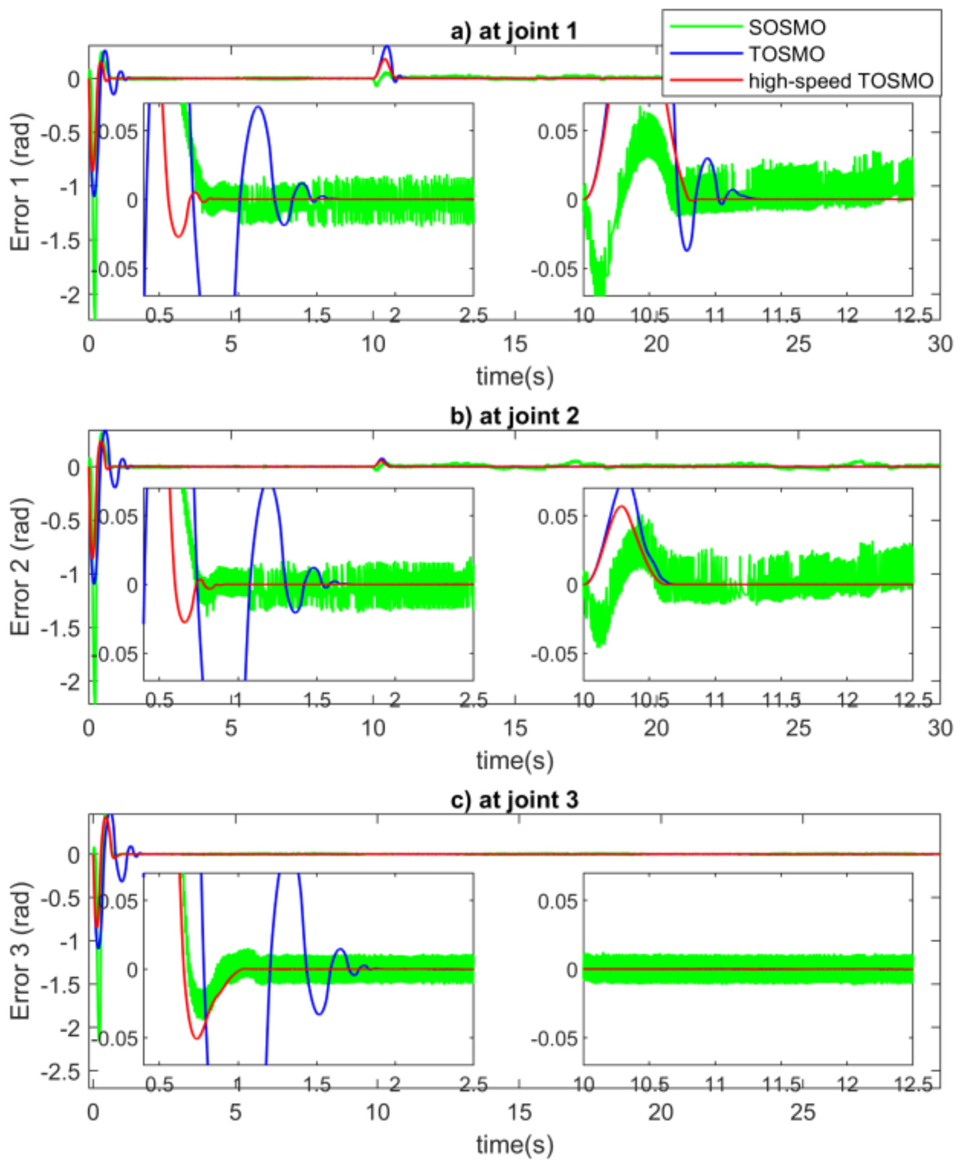
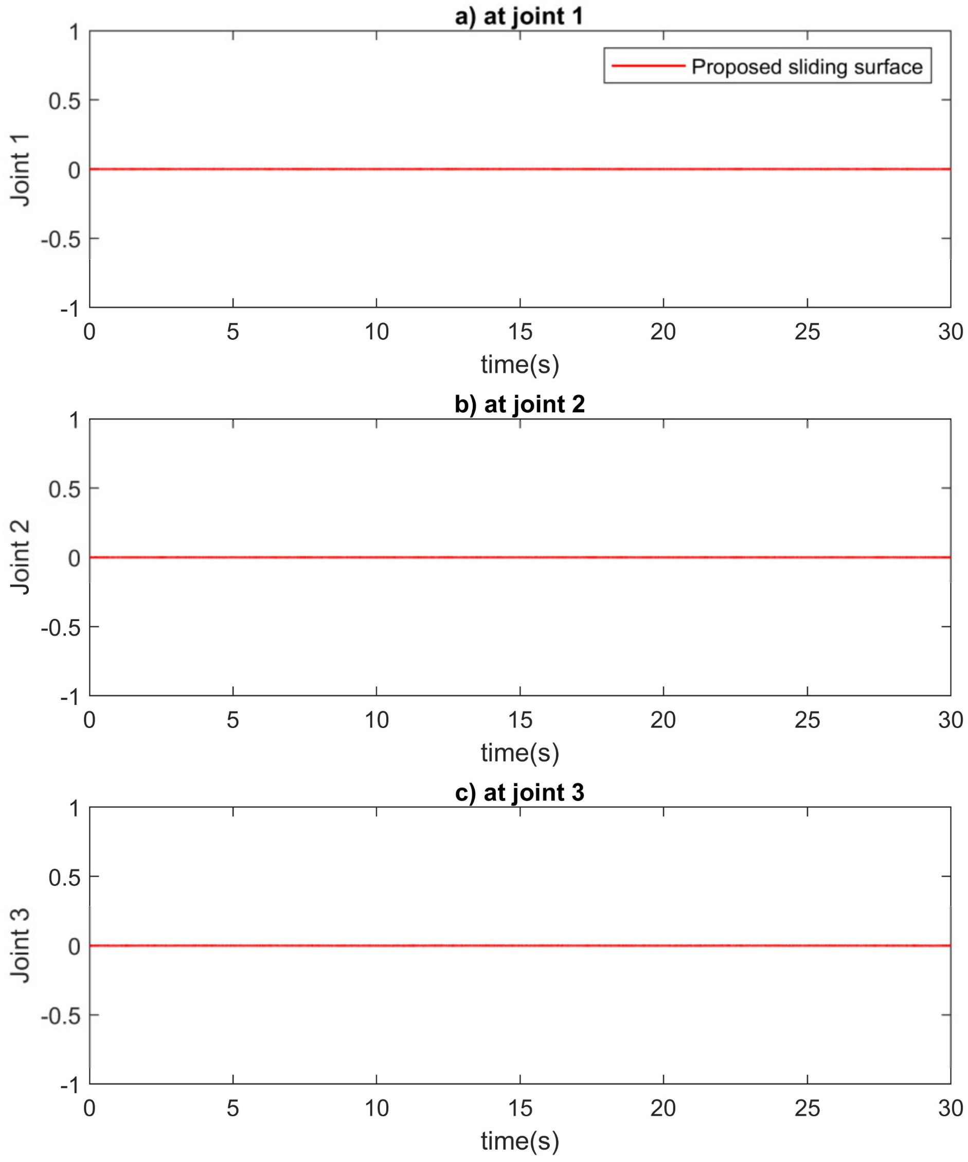
5. Numerical Simulations

To validate the efficiency of the suggested algorithm, in this section, we used the PUMA560 robot manipulator with the last three joints blocked for a computer simulation. The structure of the PUMA560 robot is shown in Figure 2. The specific parameter values of the PUMA560 robot dynamic model were provided in [50]. In the simulation analysis, the MATLAB/Simulink program was used with a sampling time of ${10}^{-3}$ s.

In the simulation, the desired trajectories of the three were assumed as

$$q_d=\left[\begin{array}{c}{q}_{d_1}\\ q_{d_2}\\ q_{d_3}\end{array}\right]=\left[\begin{array}{c}\cos \left(\pi t/5\right)-1\\ \sin \left(\pi t/5+\pi /2\right)-1\\ \sin \left(\pi t/5+\pi /2\right)-1\end{array}\right]$$

The initial states of the robot were selected as $q_1(0)=q_2(0)=q_3(0)=-0.5$ and ${\dot{q}}_1(0)={\dot{q}}_2(0)={\dot{q}}_3(0)=0$.

The friction vector and external disturbance vector were assumed as

$$\begin{gathered} F_r=\left[\begin{array}{c}{F}_{r1}\\ F_{r2}\\ F_{r3}\end{array}\right]=\left[\begin{array}{c}1.9\sin \left({\dot{q}}_1\right)\\ 2.03\sin \left({\dot{q}}_2\right)\\ 1.76\sin \left({\dot{q}}_3\right)\end{array}\right] \\ {\tau }_d=\left[\begin{array}{c}{\tau }_{d_1}\\ {\tau }_{d_2}\\ {\tau }_{d_3}\end{array}\right]=\left[\begin{array}{c}1.1{\dot{q}}_1+1.2\sin \left(3q_1\right)\\ 1.65{\dot{q}}_2+2.14\sin \left(2q_2\right)\\ -3.01{\dot{q}}_3+1.3\sin \left(q_3\right)\end{array}\right] \end{gathered}$$

The fault was assumed to occur at $T_f=10 \mathrm{s}$, with the fault signal as follows:

$$\mathrm{\Phi }=\left[\begin{array}{c}{\mathrm{\Phi }}_1\\ {\mathrm{\Phi }}_2\\ {\mathrm{\Phi }}_3\end{array}\right]=\left[\begin{array}{c}10\sin (q_1{q}_2)+3.7\cos \left({\dot{q}}_1{q}_2\right)+5.2\cos \left({\dot{q}}_1{\dot{q}}_2\right)\\ 15\sin (q_1{q}_2)+3.6\cos \left({\dot{q}}_1{q}_2\right)+2.7\cos \left({\dot{q}}_1{\dot{q}}_2\right)\\ 0\end{array}\right]$$

The parameters of the controllers and observers were selected as follows: ${\gamma }_1=1/2, {\gamma }_2=2/3$, ${\beta }_1=diag\left(15,15,15\right)$, ${\beta }_2=diag\left(10,10,10\right)$, ${\beta }_3=diag\left(10,10,10\right)$, ${\beta }_4=diag\left(5,5,5\right)$, ${\mathrm{\Delta }}_{\delta }=0.5$, $\overline{\mathrm{\Delta }}=22$, $\mu =0.01$ and $\mathrm{\Gamma }=5$.

The simulation consisted of two parts: First, the estimation results of the proposed high-speed TOSMO were compared with that of the TOSMO and the SOSMO, which were designed as in [42]. Second, the proposed fault-tolerant technique was compared with three controllers: (1) NFTSMC without compensation; (2) NFTSMC with the SOSMO compensation (NFTSMC-SOSMO); (3) NFTSMC with the TOSMO compensation (NFTSMC-TOSMO).

In the first part, the comparison results among three observers are shown in Figure 3, Figure 4 and Figure 5. The obtained velocity estimation errors are shown in Figure 3. As in the results, the SOSMO (green solid line) provided a faster estimation of velocity compared to the TOSMO (blue solid line). In contrast, the TOSMO provided a velocity estimation with higher precision and less chattering compared to the SOSMO. The red solid line in the figure shows the estimation results of the high-speed TOSMO. It was easy to see that the estimated information of the high-speed TOSMO maintained the higher precision and lesser chattering characteristic of the TOSMO, while the convergence speed was significantly increased and matched the speed of the SOSMO. The faster velocity estimation would help the controller reach a faster convergence time. In terms of the lumped unknown input estimation, the results are shown in Figure 4 and Figure 5. As shown in the results, the SOSMO provided estimation information with a lower accuracy compared to the TOSMO and the proposed high-speed TOSMO due to the time delay when using a lowpass filter to reconstruct the estimation signal. On the contrary, the TOSMO and the high-speed TOSMO could reconstruct the lumped unknown input directly without any filtration. However, the convergence time of the TOSMO was a little slower. The same applied to the velocity estimation results, where the lumped unknown input estimation results of the high-speed TOSMO could maintain the high estimation performance of the TOSMO and reached the convergence speed of the SOSMO. It is worth mentioning that the faster estimation speed helped in early fault detection, thus, reducing the robot’s failure rate.

In the second part, the comparison results among four controllers were shown in Figure 6 and Figure 7. Figure 6 shows the results of the tracking error at each joint. As in the figure, in terms of the tracking performance, NFTSMC without compensation (green solid line) and the NFTSMC-SOSMO (black dash line) provided quite good tracking precision. However, with better approximation information, the NFTSMC-TOSMO (blue solid line) and the proposed fault-tolerant control strategy (red solid line) provided higher control performance. The two controllers provided almost the same tracking accuracy due to the estimation accuracy of the TOSMO and the high-speed TOSMO being not much different. In terms of the convergence speed, NFTSMC without compensation and the NFTSMC-TOSMO converged simultaneously because they used the same velocity signal in the design process. According to the effect of the velocity signal, the proposed fault-tolerant control strategy converged faster compared to the above two controllers, and almost the same as the NFTSMC-SOSMO. Therefore, it could be concluded that the proposed high-speed TOSMO not only obtained estimation information faster, but also helped the designed controller achieve better control performance. The comparison of control input torque is shown in Figure 7. As in the figure, the control input of NFTSMC without compensation was under the effect of the chattering phenomenon because of using a large sliding gain. After compensation, the sliding gain could be chosen with a smaller value; therefore, the chattering phenomenon in the control inputs of the NFTSMC-SOSMO, the NFTSMC-TOSMO and the proposed fault-tolerant control were significantly reduced. The time response of the proposed NFTS surface is shown in Figure 8.

6. Conclusions

This paper proposed a novel fault-tolerant control strategy for robot manipulator systems using only position measurements. Thanks to the linear characteristic of the added elements, the proposed high-speed TOSMO could estimate both the velocity signal and the lumped unknown input with a faster convergence time compared to the TOSMO. The obtained information from the observer was combined with NFTSMC in designing the fault-tolerant controller. The proposed controller–observer tactic provided excellent properties, such as a fast convergence time, high-position tracking precision, finite-time convergence, chattering phenomenon reduction, robustness against the effects of the lumped unknown input and velocity requirement elimination. The faster convergence characteristic of the observer also improved the convergence speed of the designed controller. The system stability and finite-time convergence were proved using the Lyapunov stability theory. Finally, the efficiency of the proposed algorithm was validated with simulations on the PUMA560 robot manipulator. Due to the efficiency of the proposed algorithm, it would be possible to implement it in real robot system in the future. In addition, designing a fixed-time observer based on the proposed high-speed TOSMO is a promising idea.

References

1. Jin, L.; Li, S.; Yu, J.; He, J. Robot manipulator control using neural networks: A survey. Neurocomputing 2018, 285, 23–34. [Google Scholar] [CrossRef]
2. Zhang, S.; Dong, Y.; Ouyang, Y.; Yin, Z.; Peng, K. Adaptive neural control for robotic manipulators with output constraints and uncertainties. IEEE Trans. Neural Netw. Learn. Syst. 2018, 29, 5554–5564. [Google Scholar] [CrossRef] [PubMed]
3. Madsen, E.; Rosenlund, O.S.; Brandt, D.; Zhang, X. Adaptive feedforward control of a collaborative industrial robot manipulator using a novel extension of the Generalized Maxwell-Slip friction model. Mech. Mach. Theory 2021, 155, 104109. [Google Scholar] [CrossRef]
4. Nubert, J.; Köhler, J.; Berenz, V.; Allgöwer, F.; Trimpe, S. Safe and fast tracking on a robot manipulator: Robust mpc and neural network control. IEEE Robot. Autom. Lett. 2020, 5, 3050–3057. [Google Scholar] [CrossRef]
5. Xie, Z.; Jin, L.; Luo, X.; Hu, B.; Li, S. An Acceleration-Level Data-Driven Repetitive Motion Planning Scheme for Kinematic Control of Robots With Unknown Structure. IEEE Trans. Syst. Man Cybern. Syst. 2021, 52, 5679–5691. [Google Scholar] [CrossRef]
6. Fan, J.; Jin, L.; Xie, Z.; Li, S.; Zheng, Y. Data-driven motion-force control scheme for redundant manipulators: A kinematic perspective. IEEE Trans. Ind. Inform. 2021, 18, 5338–5347. [Google Scholar] [CrossRef]
7. Van, M.; Do, X.P.; Mavrovouniotis, M. Self-tuning fuzzy PID-nonsingular fast terminal sliding mode control for robust fault tolerant control of robot manipulators. ISA Trans. 2020, 96, 60–68. [Google Scholar] [CrossRef]
8. Vo, A.T.; Kang, H.-J.; Nguyen, V.-C. An output feedback tracking control based on neural sliding mode and high order sliding mode observer. In Proceedings of the 2017 10th International Conference on Human System Interactions (HSI), Ulsan, Korea, 17–19 July 2017; pp. 161–165. [Google Scholar]
9. Song, Y.; Huang, X.; Wen, C. Robust adaptive fault-tolerant PID control of MIMO nonlinear systems with unknown control direction. IEEE Trans. Ind. Electron. 2017, 64, 4876–4884. [Google Scholar] [CrossRef]
10. Alibeji, N.; Sharma, N. A PID-Type Robust Input Delay Compensation Method for Uncertain Euler—Lagrange Systems. IEEE Trans. Control Syst. Technol. 2017, 25, 2235–2242. [Google Scholar] [CrossRef]
11. Tutsoy, O.; Barkana, D.E. Model free adaptive control of the under-actuated robot manipulator with the chaotic dynamics. ISA Trans. 2021, 118, 106–115. [Google Scholar] [CrossRef]
12. Muñoz-Vázquez, A.J.; Treesatayapun, C. Model-free discrete-time fractional fuzzy control of robotic manipulators. J. Frankl. Inst. 2022, 359, 952–966. [Google Scholar] [CrossRef]
13. Song, Y.; Guo, J. Neuro-adaptive fault-tolerant tracking control of Lagrange systems pursuing targets with unknown trajectory. IEEE Trans. Ind. Electron. 2017, 64, 3913–3920. [Google Scholar] [CrossRef]
14. Nguyen, V.-C.; Vo, A.-T.; Kang, H.-J. Continuous PID Sliding Mode Control Based on Neural Third Order Sliding Mode Observer for Robotic Manipulators. In Proceedings of the International Conference on Intelligent Computing, Nanchang, China, 3–6 August 2019; pp. 167–178. [Google Scholar]
15. Cheng, X.; Liu, H.; Lu, W. Chattering-Suppressed Sliding Mode Control for Flexible-Joint Robot Manipulators. Actuators 2021, 10, 288. [Google Scholar] [CrossRef]
16. Zhou, W.; Wang, Y.; Liang, Y. Sliding mode control for networked control systems: A brief survey. ISA Trans. 2021, 124, 249–259. [Google Scholar] [CrossRef]
17. Alwi, H.; Edwards, C. Fault detection and fault-tolerant control of a civil aircraft using a sliding-mode-based scheme. IEEE Trans. Control Syst. Technol. 2008, 16, 499–510. [Google Scholar] [CrossRef]
18. Utkin, V.I. Sliding Modes in Control and Optimization; Springer Science & Business Media: New York, NY, USA, 2013. [Google Scholar]
19. Yu, S.; Yu, X.; Shirinzadeh, B.; Man, Z. Continuous finite-time control for robotic manipulators with terminal sliding mode. Automatica 2005, 41, 1957–1964. [Google Scholar] [CrossRef]
20. Zhihong, M.; Paplinski, A.P.; Wu, H.R. A robust MIMO terminal sliding mode control scheme for rigid robotic manipulators. IEEE Trans. Automat. Control 1994, 39, 2464–2469. [Google Scholar] [CrossRef]
21. Islam, S.; Liu, X.P. Robust sliding mode control for robot manipulators. IEEE Trans. Ind. Electron. 2010, 58, 2444–2453. [Google Scholar] [CrossRef]
22. Nguyen, V.-C.; Le, P.-N.; Kang, H.-J. Model-Free Continuous Fuzzy Terminal Sliding Mode Control for Second-Order Nonlinear Systems. In Proceedings of the International Conference on Intelligent Computing, Shenzhen, China, 12–15 August 2021; pp. 245–258. [Google Scholar]
23. Xu, Q. Piezoelectric nanopositioning control using second-order discrete-time terminal sliding-mode strategy. IEEE Trans. Ind. Electron. 2015, 62, 7738–7748. [Google Scholar] [CrossRef]
24. Truong, T.N.; Vo, A.T.; Kang, H.-J. Implementation of an Adaptive Neural Terminal Sliding Mode for Tracking Control of Magnetic Levitation Systems. IEEE Access 2020, 8, 206931–206941. [Google Scholar] [CrossRef]
25. Mobayen, S. Fast terminal sliding mode controller design for nonlinear second-order systems with time-varying uncertainties. Complexity 2015, 21, 239–244. [Google Scholar] [CrossRef]
26. Cruz-Ortiz, D.; Chairez, I.; Poznyak, A. Non-singular terminal sliding-mode control for a manipulator robot using a barrier Lyapunov function. ISA Trans. 2022, 121, 268–283. [Google Scholar] [CrossRef] [PubMed]
27. Shao, X.; Sun, G.; Xue, C.; Li, X. Nonsingular terminal sliding mode control for free-floating space manipulator with disturbance. Acta Astronaut. 2021, 181, 396–404. [Google Scholar] [CrossRef]
28. Zaare, S.; Soltanpour, M.R. Continuous fuzzy nonsingular terminal sliding mode control of flexible joints robot manipulators based on nonlinear finite time observer in the presence of matched and mismatched uncertainties. J. Frankl. Inst. 2020, 357, 6539–6570. [Google Scholar] [CrossRef]
29. Nguyen, V.-C.; Kang, H.-J. A Fault Tolerant Control for Robotic Manipulators Using Adaptive Non-singular Fast Terminal Sliding Mode Control Based on Neural Third Order Sliding Mode Observer. In Proceedings of the International Conference on Intelligent Computing, Sanya, China, 4–6 December 2020; pp. 202–212. [Google Scholar]
30. Vo, A.T.; Kang, H.-J. A novel fault-tolerant control method for robot manipulators based on non-singular fast terminal sliding mode control and disturbance observer. IEEE Access 2020, 8, 109388–109400. [Google Scholar] [CrossRef]
31. Nguyen, V.-C.; Le, P.-N.; Kang, H.-J. An Active Fault-Tolerant Control for Robotic Manipulators Using Adaptive Non-Singular Fast Terminal Sliding Mode Control and Disturbance Observer. Actuators 2021, 10, 332. [Google Scholar] [CrossRef]
32. Utkin, V.; Guldner, J.; Shi, J. Sliding Mode Control in Electro-Mechanical Systems; CRC Press: Boca Raton, FL, USA, 2009. [Google Scholar]
33. Zhou, Q.; Shi, P.; Xu, S.; Li, H. Observer-based adaptive neural network control for nonlinear stochastic systems with time delay. IEEE Trans. Neural Netw. Learn. Syst. 2012, 24, 71–80. [Google Scholar] [CrossRef]
34. Abdollahi, F.; Talebi, H.A.; Patel, R. V A stable neural network-based observer with application to flexible-joint manipulators. IEEE Trans. Neural Netw. 2006, 17, 118–129. [Google Scholar] [CrossRef]
35. Ya-Li, D.; Sheng-Wei, M.E.I. Adaptive observer for a class of nonlinear systems. Acta Autom. Sin. 2007, 33, 1081–1084. [Google Scholar]
36. Jiang, B.; Staroswiecki, M.; Cocquempot, V. Fault diagnosis based on adaptive observer for a class of non-linear systems with unknown parameters. Int. J. Control 2004, 77, 367–383. [Google Scholar] [CrossRef]
37. Wang, Y.; Leibold, M.; Lee, J.; Ye, W.; Xie, J.; Buss, M. Incremental Model Predictive Control Exploiting Time-Delay Estimation for a Robot Manipulator. IEEE Trans. Control Syst. Technol. 2022, 1–16, (Early Access). [Google Scholar] [CrossRef]
38. Van, M.; Ge, S.S.; Ren, H. Finite Time Fault Tolerant Control for Robot Manipulators Using Time Delay Estimation and Continuous Nonsingular Fast Terminal Sliding Mode Control. IEEE Trans. Cybern. 2017, 47, 1681–1693. [Google Scholar] [CrossRef] [PubMed]
39. Wang, X.; Liao, R.; Shi, C.; Wang, S. Linear extended state observer-based motion synchronization control for hybrid actuation system of more electric aircraft. Sensors 2017, 17, 2444. [Google Scholar] [CrossRef] [PubMed]
40. Saleki, A.; Fateh, M.M. Model-free control of electrically driven robot manipulators using an extended state observer. Comput. Electr. Eng. 2020, 87, 106768. [Google Scholar] [CrossRef]
41. Van, M.; Kang, H.-J.; Suh, Y.-S. A novel neural second-order sliding mode observer for robust fault diagnosis in robot manipulators. Int. J. Precis. Eng. Manuf. 2013, 14, 397–406. [Google Scholar] [CrossRef]
42. Nguyen, V.-C.; Vo, A.-T.; Kang, H.-J. A Non-singular Fast Terminal Sliding Mode Control Based on Third-Order Sliding Mode Observer for a Class of Second-Order Uncertain Nonlinear Systems and Its Application to Robot Manipulators. IEEE Access 2020, 8, 78109–78120. [Google Scholar] [CrossRef]
43. Nguyen, V.-C.; Vo, A.-T.; Kang, H.-J. A Finite-Time Fault-Tolerant Control Using Non-Singular Fast Terminal Sliding Mode Control and Third-Order Sliding Mode Observer for Robotic Manipulators. IEEE Access 2021, 9, 31225–31235. [Google Scholar] [CrossRef]
44. Feng, Y.; Han, F.; Yu, X. Chattering free full-order sliding-mode control. Automatica 2014, 50, 1310–1314. [Google Scholar] [CrossRef]
45. Van, M.; Ge, S.S.; Ren, H. Robust fault-tolerant control for a class of second-order nonlinear systems using an adaptive third-order sliding mode control. IEEE Trans. Syst. Man Cybern. Syst. 2016, 47, 221–228. [Google Scholar] [CrossRef]
46. Tran, X.-T.; Kang, H.-J. Continuous adaptive finite-time modified function projective lag synchronization of uncertain hyperchaotic systems. Trans. Inst. Meas. Control 2018, 40, 853–860. [Google Scholar] [CrossRef]
47. Levant, A. Higher-order sliding modes, differentiation and output-feedback control. Int. J. Control 2003, 76, 924–941. [Google Scholar] [CrossRef]
48. Ortiz-Ricardez, F.A.; Sánchez, T.; Moreno, J.A. Smooth Lyapunov function and gain design for a second order differentiator. In Proceedings of the 2015 54th IEEE Conference on Decision and Control (CDC), Osaka, Japan, 15–18 December 2015; pp. 5402–5407. [Google Scholar]
49. Tran, X.-T.; Kang, H.-J. A Novel Adaptive Finite-Time Control Method for a Class of Uncertain Nonlinear Systems. Int. J. Precis. Eng. Manuf. 2015, 16, 2647–2654. [Google Scholar] [CrossRef]
50. Armstrong, B.; Khatib, O.; Burdick, J. The explicit dynamic model and inertial parameters of the PUMA 560 arm. In Proceedings of the 1986 IEEE International Conference on Robotics and Automation, San Francisco, CA, USA, 7–10 April 1986; Volume 3, pp. 510–518. [Google Scholar]
Figure 1. Overall structure of the proposed fault-tolerant control approach.
Actuators 11 00259 g001
Figure 2. Structure of the PUMA560 robot manipulator.
Actuators 11 00259 g002
Figure 3. Velocity estimation errors at (a) joint 1, (b) joint 2 and (c) joint 3.
Actuators 11 00259 g003
Figure 4. Lumped unknown input estimation at (a) joint 1, (b) joint 2 and (c) joint 3.
Actuators 11 00259 g004
Figure 5. Lumped unknown input estimation errors at (a) joint 1, (b) joint 2 and (c) joint 3.
Actuators 11 00259 g005
Figure 6. Comparison of tracking errors among controllers at (a) joint 1, (b) joint 2 and (c) joint 3.
Actuators 11 00259 g006
Figure 7. Comparison of control input torque among controllers at (a) joint 1, (b) joint 2 and (c) joint 3.
Actuators 11 00259 g007
Figure 8. Time response of the proposed sliding surface at (a) joint 1, (b) joint 2 and (c) joint 3.
Actuators 11 00259 g008
Publisher’s Note: MDPI stays neutral with regard to jurisdictional claims in published maps and institutional affiliations.