Admissible Control for Non-Linear Singular Systems Subject to Time-Varying Delay and Actuator Saturation: An Interval Type-2 Fuzzy Approach

Abstract

Applied in many fields, nonlinear systems involving delay and algebraic equations are referred to as singular systems. These systems remain challenging due to saturation constraints that affect actuators and cause harm to their operation. Furthermore, the complexity of the problem will increase when uncertainty also simultaneously affects the system under consideration. To address this issue, this paper investigated a feasible control strategy for nonlinear singular systems with time-varying delay that are subject to uncertainty and actuator saturation. The IT-2 fuzzy model was adopted to describe the dynamic of the non-linear delayed systems using lower and upper membership functions to deal with the uncertainty. Moreover, the polyhedron model was applied to characterize the saturation function. The goal of the control approach was to design a relevant IT2 fuzzy state feedback controller with mismatched membership functions so that the closed-loop system is admissible. On the basis of an appropriate Lyapunov–Krasovskii functional, sufficient delay-dependent conditions were established and an optimization problem was formulated in terms of linear matrix inequality constraints to optimize the attraction domain. Simulation examples are provided to verify the effectiveness of the proposed method.

1. Introduction

This section includes the literature review, notations, and acronyms used in the document, as well as an outline of the publication and its goals.

1.1. Literature Review

Singular systems that are described by a couple of algebraic and differential equations are characterized by their different modes, namely finite dynamic modes, infinite nondynamic modes, and infinite dynamic modes, respectively. The infinite dynamic modes have the feature to destroy the stability and performance of the system. Thus, the admissibility, which includes stability, regularity, and non-impulsiveness/causality, should be verified when dealing with this class of systems. As a consequence, the investigation of singular systems is both theoretically and practically important [1,2]. It is worth noting that time delays are common in many physical plants, and they can have a substantial negative impact on the performance and even the stability of practical systems [3,4,5,6,7]. Singular models and time-delay phenomena are general enough to enable some fundamental results from the theory of state-space systems to be extended to this class of systems (see, for instance, [8,9,10,11,12]). Alternatively, it is widely known that all physical plants are affected by the actuator and/or sensor saturation. The saturation constraint has a nonlinear impact on the performance of the controlled system unless the controller is built to account for it. In addition, ignorance of the consequences of actuator saturation may destroy system stability. Control with input/output saturation has been subjected to a great deal of research and development over the last decade [13,14,15,16,17].

In general, the research on nonlinear systems [18] is an extremely hard issue due to their inherent complexity. Due to its rigorous mathematical structure, the fuzzy model has recently been applied to handle nonlinear complex systems, since this model is known for its powerful approximation of smoothly nonlinear systems [19,20,21]. In the research on nonlinear singular systems against input saturation, the fuzzy method has thus far proven useful, including the finite-time output feedback control for fuzzy singular system with actuator saturation [22], the fault-tolerant sliding mode control for fuzzy systems with time-varying delay and actuator saturation [23], the stabilization of the descriptor systems against input saturation [24], and the fuzzy dissipative controller design for non-linear descriptor systems subject to time-delay and actuator saturation [25].

In many cases, uncertainty arises, such as partially unknown parameters, unpredictable disturbances in the system, varying interpretations of linguistic variables of the fuzzy models, etc. It is worth noting, however, that the membership functions of type-1 fuzzy sets are well-known, and the control problem cannot be handled directly for nonlinear plants with parameter uncertainties. As type-1 fuzzy sets have limitations in dealing with non-linear plants subject to parameter uncertainties, the IT-2 fuzzy model was proposed and used in [26,27]. Research on IT-2 fuzzy systems has attracted attention due to the advantages of IT-2 fuzzy sets over type-1 fuzzy sets in dealing with parameter uncertainties, and many control design results have been developed [28,29,30]. To mention a few, in [31], fuzzy decentralized output feedback control was investigated using the event-triggered approach for interval type-2 fuzzy systems against input saturation. The study in [32] discussed the issue of filter design for IT-2 fuzzy systems with D-stability constraints. The authors in [33] investigated discrete-time interval-valued fuzzy systems with actuator faults to study the reliable non-fragile control problem with performance. When the system is subject to stochastic network delays and actuator saturation, a distributed-delay-dependent method was proposed in [34] for stabilizing interval type-2 Takagi–Sugeno fuzzy systems. Under saturated state feedback, robust stabilization was investigated in [35] for uncertain linear systems with discrete and distributed delays.

Very recently, the IT-2 fuzzy approach was extended to non-linear singular systems with uncertainties. To mention a few, admissibilization for IT-2 fuzzy singular systems was studied in [36]. Based on the LMI approach, the dynamic output-feedback control design issue was investigated in [37] for singular interval-valued fuzzy systems.

There is a need to emphasize that the previous papers discussed various fuzzy stabilization problems for IT-2 fuzzy singular systems without simultaneously considering the phenomenon of input saturation. In light of this, we undertook this study. Furthermore, although some related results have recently been published for delayed nonlinear systems characterized by IT-2 fuzzy models [38,39], they cannot be applied to nonlinear singular systems. This paper attempts to overcome the deficiencies of the aforementioned studies by dealing with the stabilization problem for input-saturated IT-2 fuzzy singular systems while simultaneously taking into account that uncertainty and delay may affect the process.

1.2. Objective and Outline

This study has the following main objectives:

(i)

Instead of existing control schemes developed for type-1 fuzzy singular systems with delay and actuator saturation [40], this study explored state feedback controllers based on IT-2 fuzzy rules in order to handle uncertain non-linear singular systems.

(ii)

The delay property and actuator saturation for the IT-2 fuzzy singular system under consideration were simultaneously considered in this study. Moreover, compared with the results suggested in [36,41], a more realistic problem was investigated in this paper that cannot be solved by the methods in the previous references.

(iii)

A new Lyapunov–Krasovskii functional candidate was constructed, and the delay-range-dependent approach was adopted to derive an admissibilization criterion via LMI formulation. Furthermore, the domain of attraction of the origin can be estimated for the underlying system.

After outlining the introduction and the objectives of our study, the paper is organized as follows: Section 2 presents the model and assumptions, as well as a description of the problem under study. In Section 3, we present and discuss the main findings of the paper. Specifically, this section is dedicated to developing a new delay-dependent admissibility criterion using the IT-2 fuzzy model from (3) and selecting a suitable Lyapunov–Krasovskii functional. To further ensure the usage of this scheme, we developed an LMI criterion to establish that the closed-loop system is admissible and to optimize the attraction domain. To demonstrate the potential applications of the proposed scheme and validate its effectiveness, numerical simulations on mass–spring–damper and inverted pendulum systems are presented in Section 4. Lastly, we conclude with some conclusions regarding the obtained results, as well as some suggestions for future research in Section 5.

1.3. Notations

Table 1. List of notations and acronyms used in the paper.

Symbol	Acronym/Notation
ℝ	set of the real numbers
$\mathcal{X}\in {\mathrm{ℝ}}^n$	n-dimensional Euclidean space
$\mathit{X}\in {\mathrm{ℝ}}^{n\times m}$	$n\times m$ real matrix
$\mathit{X}>0$	real symmetric positive definite matrix $\mathit{X}$
$\parallel \mathit{X}\parallel$	norm of the matrix $\mathit{X}$
${\mathit{X}}^{\top }$	transpose of the matrix $\mathit{X}$
$\mathrm{sym}\left(\mathit{X}\right)$	$\mathit{X}+{\mathit{X}}^{\top }$
$\lambda \left(\right)$	eigenvalue of a matrix
${\parallel \varphi \parallel }_c$	${max}_{\alpha \in [-d_2,0]}\parallel \mathbf{\varphi }\left(\alpha \right)\parallel$
$\parallel \dot{\varphi }{\parallel }_c$	${max}_{\alpha \in [-d_2,0]}\parallel \dot{\mathbf{\varphi }}\left(\alpha \right)\parallel$
*	term that is induced by symmetry
r	number of if-then rules
LMI	linear matrix inequalities
IT-2	Interval type-2 fuzzy model
TS	Takagi–Sugeno

lists the notations and acronyms that should be used in this study.

2. Preliminaries and Problem Statement

The aim of this section is to introduce some preliminaries that facilitate the understanding of our proposal and state the problem that we are investigating.

2.1. IT-2 TS Fuzzy Model

Consider a class of non-linear singular systems that can be described by the following IT-2 TS fuzzy model:

$$\begin{array}{cc}\hfill & {\mathit{R}}_i:\mathrm{If}{\theta }_1\left(\mathit{x}\left(t\right)\right)\mathrm{is}{\mathcal{M}}_i^1\mathrm{and}\mathrm{If}{\theta }_2\left(\mathit{x}\left(t\right)\right)\mathrm{is}{\mathcal{M}}_i^2\cdots \mathrm{If}{\theta }_s\left(\mathit{x}\left(t\right)\right)\mathrm{is}{\mathcal{M}}_i^s,\mathrm{Then}\hfill \\ & \left\{\begin{array}{cc}\hfill \mathit{E}\dot{\mathit{x}}\left(t\right)& ={\mathit{A}}_i\mathit{x}\left(t\right)+{\mathit{A}}_{di}\mathit{x}(t-d\left(t\right))+{\mathit{B}}_i\mathbf{\sigma }\left(\mathit{u}\left(t\right)\right)\hfill \\ \hfill \mathit{x}\left(t\right)& =\mathbf{\varphi }\left(t\right),\forall t\in [-d_{2}0],\hfill \end{array}\right.\hfill \end{array}$$

(1)

where ${\mathcal{M}}_i^k$ is an IT-2 fuzzy set of rule i corresponding to the premise variable ${\theta }_i\left(\mathit{x}\left(t\right)\right)$, $k=1,2,\cdots ,s$, k is the number of premise variables, and $i\in \mathrm{𝕊}\triangleq \{1,2,\dots ,r\}$ is the number of rules. $\mathit{x}\left(t\right)\in {\mathit{R}}^n$ and $\mathbf{\sigma }\left(\mathit{u}\left(t\right)\right)\in {\mathit{R}}^m$ define, respectively, the state and saturated input vectors. Matrices ${\mathit{A}}_i$, ${\mathit{A}}_{di}$ and ${\mathit{B}}_i$ in model (1) are known with appropriate dimensions. $d\left(t\right)$ stands for the time-varying delay, and $\mathbf{\varphi }\left(t\right)$ defines the initial state for all $t\in [-d_{2}0]$.

2.2. Assumptions and Resulting Model

A1

$d\left(t\right)$ is a continuous function such that

$$\begin{array}{c}\hfill 0<d_1\le d\left(t\right)\le d_2,0\le \dot{d}\left(t\right)\le d_r\end{array}$$

(2)

where $d_1$ represents the lower delay bound, $d_2$ stands for the upper delay bound, and $d_r$ is the delay variation rate.

A2

Singular matrix $\mathit{E}$ satisfies $rank\left(\mathit{E}\right)=q<n$.

A3

$\mathbf{\sigma }\left(\mathit{u}\right(t\left)\right)$ is the saturation that affects the actuator according to the following model:

$$\begin{array}{cc}\hfill \mathbf{\sigma }\left(\mathit{u}\right(t\left)\right)& ={\left[\begin{array}{cccc}\sigma \left(u_1\left(t\right)\right)& \sigma \left(u_2\left(t\right)\right)& \cdots & \sigma \left(u_m\left(t\right)\right)\end{array}\right]}^{\top }\hfill \\ \hfill \sigma \left(u_l\left(t\right)\right)& =\left\{\begin{array}{cc}{\overline{u}}_l\hfill & \mathrm{if}{u}_l\left(t\right)>{\overline{u}}_l\hfill \\ u_l\left(t\right)\hfill & \mathrm{if}-{\overline{u}}_l\le u_l\left(t\right)\le {\overline{u}}_l\hfill \\ -{\overline{u}}_l\hfill & \mathrm{if}{u}_l\left(t\right)<-{\overline{u}}_l\hfill \end{array}\right.\hfill \end{array}$$

where $u_l\left(t\right)$ is the $lth$ value of $\mathit{u}\left(t\right)$, and ${\overline{u}}_l$ is the $lth$ saturated level, $l=1,\cdots ,m$.

Based on the IT-2 fuzzy approach, the following interval defines the firing strength of the ith rule:

$$\begin{array}{cc}\hfill {\mathbb{M}}_i& =\left[\begin{array}{cc}\prod _{k=1}^s{\underline{\omega }}_{{\mathcal{M}}_i^k\left(\mathbf{\theta }\left(\mathit{x}\left(t\right)\right)\right)}& \prod _{k=1}^s{\overline{\omega }}_{{\mathcal{M}}_i^k\left(\mathbf{\theta }\left(\mathit{x}\left(t\right)\right)\right)}\end{array}\right]=\left[\begin{array}{cc}{\underline{\mu }}_i\left(\mathit{x}\left(t\right)\right)& {\overline{\mu }}_i\left(\mathit{x}\left(t\right)\right)\end{array}\right]\hfill \end{array}$$

where ${\underline{\mu }}_i\left(\mathit{x}\left(t\right)\right)\ge 0$ and ${\overline{\mu }}_i\left(\mathit{x}\left(t\right)\right)\ge 0$ are, respectively, the the lower and upper membership functions, and ${\underline{\omega }}_{{\mathcal{M}}_i^k\left(\mathbf{\theta }\left(\mathit{x}\left(t\right)\right)\right)}\ge 0$, and ${\overline{\omega }}_{{\mathcal{M}}_i^k\left(\mathbf{\theta }\left(\mathit{x}\left(t\right)\right)\right)}\ge 0$ stand, respectively, for the lower and upper grades of membership. Therefore, the non-linear singular system can be described as

$$\begin{array}{cc}\hfill & \left\{\begin{array}{cc}\hfill \mathit{E}\dot{\mathit{x}}\left(t\right)& =\sum _{i=1}^r{\mu }_i\left(\mathit{x}\left(t\right)\right)\left({\mathit{A}}_i\mathit{x}\left(t\right)+{\mathit{A}}_{di}\mathit{x}(t-d\left(t\right))+{\mathit{B}}_i\sigma \left(\mathit{u}\left(t\right)\right)\right)\hfill \\ \hfill \mathit{x}\left(t\right)& =\mathbf{\varphi }\left(t\right),t\in [-d_2,0]\hfill \end{array}\right.\hfill \end{array}$$

(3)

${\mu }_i\left(\mathit{x}\left(t\right)\right)$ denotes the grade of the membership of the ith local system defined as

$$\begin{array}{ccc}\hfill {\mu }_i\left(\mathit{x}\left(t\right)\right)& ={\underline{\alpha }}_i\left(\mathit{x}\left(t\right)\right){\underline{\mu }}_i\left(\mathit{x}\left(t\right)\right)+{\overline{\alpha }}_i\left(\mathit{x}\left(t\right)\right){\overline{\mu }}_i\left(\mathit{x}\left(t\right)\right),\sum _{i=1}^r{\mu }_i\left(\mathit{x}\left(t\right)\right)\hfill & \hfill =1\end{array}$$

where ${\underline{\alpha }}_i\left(\mathit{x}\left(t\right)\right)$ and ${\overline{\alpha }}_i(\mathit{x}\left(t\right)$ are two weighting coefficient functions satisfying

$$\begin{array}{c}\hfill 0\le {\underline{\alpha }}_i\left(\mathit{x}\left(t\right)\right),{\overline{\alpha }}_i\left(\mathit{x}\left(t\right)\right)\le 1,{\underline{\alpha }}_i\left(\mathit{x}\left(t\right)\right)+{\overline{\alpha }}_i\left(\mathit{x}\left(t\right)\right)=1\end{array}$$

(4)

Note that, by introducing weighting coefficient functions, we can represent any time-variant or time-invariant unmeasured parameters of the general non-linear system. Moreover, these functions are not necessarily known but exist and satisfy (4).

As a matter of convenience, ${\mu }_i\left(\mathit{x}\left(t\right)\right)$ will be referred to as ${\mu }_i$ in the sequel.

2.3. IT-2 Fuzzy State Feedback Controller Design

Here, the subsequent IT-2 fuzzy state-feedback controller structure was adopted to admissibilize the system under consideration:

$$\begin{array}{cc}\hfill \mathrm{Controller}\mathrm{Rule}{}_j:& \mathrm{If}{\vartheta }_1\left(\mathit{x}\left(t\right)\right)\mathrm{is}{\mathcal{N}}_j^1\mathrm{and}\mathrm{If}{\vartheta }_2\left(\mathit{x}\left(t\right)\right)\mathrm{is}{\mathcal{N}}_j^2\cdots \mathrm{If}{\vartheta }_s\left(\mathit{x}\left(t\right)\right)\mathrm{is}{\mathcal{N}}_j^s,\mathrm{Then}\hfill \\ & \mathit{u}\left(t\right)={\mathit{K}}_j\mathit{x}\left(t\right)\hfill \end{array}$$

where ${\mathit{K}}_j$ is the gain matrix to be designed. Similarly, $\mathbf{\vartheta }\left(\mathit{x}\left(t\right)\right)=[{\vartheta }_1\left(\mathit{x}\left(t\right)\right),{\vartheta }_2\left(\mathit{x}\left(t\right)\right),\dots ,{\vartheta }_s$$\left(\mathit{x}\right(t\left)\right)]$ defines the premise vector, and ${\mathcal{N}}_j^{k_c},(k_c=1,2,\cdots ,s)$ represents the type-2 fuzzy sets of the j-th controller rule.

The following is the firing interval for the jth rule:

$$\begin{array}{cc}\hfill {\mathbb{N}}_j& =\left[\begin{array}{cc}{\underline{\nu }}_j\left(\mathit{x}\left(t\right)\right)& {\overline{\nu }}_j\left(\mathit{x}\left(t\right)\right)\end{array}\right],j\in \mathrm{𝕊}\hfill \end{array}$$

where

$$\begin{array}{cccc}\hfill {\underline{\nu }}_j\left(\mathit{x}\left(t\right)\right)& =\prod _{k_c=1}^s{\underline{\omega }}_{{\mathcal{N}}_j^{k_c}\left(\mathbf{\vartheta }\left(\mathit{x}\left(t\right)\right)\right)}\ge 0,\hfill & \hfill {\overline{\nu }}_j\left(\mathit{x}\left(t\right)\right)& =\prod _{k_c=1}^s{\overline{\omega }}_{{\mathcal{N}}_j^{k_c}\left(\mathbf{\vartheta }\left(\mathit{x}\left(t\right)\right)\right)}\ge 0,\hfill \end{array}$$

${\underline{\nu }}_j\left(\mathit{x}\left(t\right)\right)$ and ${\overline{\nu }}_j\left(\mathit{x}\left(t\right)\right)$ define, respectively, the lower and upper membership functions. ${\underline{\omega }}_{{\mathcal{N}}_j^{k_c}\left(\mathbf{\vartheta }\left(\mathit{x}\left(t\right)\right)\right)}\ge 0$ and ${\overline{\omega }}_{{\mathcal{N}}_j^{k_c}\left(\mathbf{\vartheta }\left(\mathit{x}\left(t\right)\right)\right)}\ge 0$ stand for the lower and upper grades of the membership of $\mathbf{\vartheta }\left(\mathit{x}\right(t\left)\right)$ in ${\mathcal{N}}_j^k$, respectively. The global fuzzy model can be inferred as follows:

$$\begin{array}{cc}\hfill \mathit{u}\left(t\right)& =\sum _{j=1}^r{\nu }_j\left(\mathit{x}\left(t\right)\right)\left({\mathit{K}}_j\mathit{x}\left(t\right)\right)\hfill \end{array}$$

(5)

$$\begin{array}{cc}\hfill & {\nu }_j\left(\mathit{x}\left(t\right)\right)={\displaystyle \frac{{\underline{\beta }}_j\left(\mathit{x}\left(t\right)\right){\underline{\nu }}_j\left(\mathit{x}\left(t\right)\right)+{\overline{\beta }}_j\left(\mathit{x}\left(t\right)\right){\overline{\nu }}_j\left(\mathit{x}\left(t\right)\right)}{{\displaystyle \sum _{l=1}^r}({\underline{\beta }}_l\left(\mathit{x}\left(t\right)\right){\underline{\nu }}_l\left(\mathit{x}\left(t\right)\right)+{\overline{\beta }}_l\left(\mathit{x}\left(t\right)\right){\overline{\nu }}_l\left(\mathit{x}\left(t\right)\right))}},{\nu }_j\left(\mathit{x}\left(t\right)\right)\ge 0,\sum _{j=1}^r{\nu }_j\left(\mathit{x}\left(t\right)\right)=1\hfill \end{array}$$

(6)

Remark 1.

Over the past several decades, type-1 fuzzy systems have been extensively investigated. It is interesting to note that all of these studies are founded on the PDC approach, in which the controller and the plant both have the same membership functions. Nevertheless, this assumption is not always valid since membership functions may be uncertain in practice. As proposed in [36,41], we aim to address this issue using the interval-valued type-2 fuzzy controller (5).

From (5), the fuzzy-model-based actuator saturation control input is expressed as:

$$\begin{array}{cc}\hfill \mathbf{\sigma }\left(\mathit{u}\right(t\left)\right)& =\mathbf{\sigma }\left(\sum _{j=1}^r{\nu }_j\left(\mathit{x}\left(t\right)\right){\mathit{K}}_j\mathit{x}\left(t\right)\right)\hfill \end{array}$$

(7)

To deal with the saturation function, the following lemmas should be provided for further development.

Definition 1.

• For a positive scalar ρ, an ellipsoid set is defined as

  $$\begin{array}{c}\hfill \epsilon ({\mathit{E}}^{\top }\mathit{P}\mathit{E},\rho )=\{x\in {\mathit{R}}^n;{\mathit{x}}^{\top }{\mathit{E}}^{\top }\mathit{P}\mathit{E}x\le \rho \},\end{array}$$

  where ${\mathit{E}}^{\top }\mathit{P}\mathit{E}$ defines a positive definite matrix.
• For a given matrix $\mathit{H}\in {\mathrm{ℝ}}^{m\times n}$, a polyhedral set is given by

  $$\begin{array}{c}\hfill \mathcal{L}(\mathit{H},\overline{u})=\{x\in {\mathit{R}}^n;|H_{l}x|\le {\overline{u}}_l,l=1,\dots ,m\},\end{array}$$

  where $H_l$ represents the lth row of $\mathit{H}$, and ${\overline{u}}_l$ is a positive given scalar.

Lemma 1

([40]). For given matrices $\mathit{K},\mathit{H}\in {\mathit{R}}^{m\times n}$, if $\mathit{x}\in \mathcal{L}(\mathit{H},\overline{\mathit{u}})$, then

$$\begin{array}{c}\hfill \sigma (\mathit{K}\mathit{x},\overline{u})=co\left\{{\mathit{M}}_s\mathit{K}+{\mathit{M}}_s^{-}\mathit{H},s\in [1,\varsigma ]\right\};\varsigma =2^m\end{array}$$

where $\mathit{x}\in {\mathrm{ℝ}}^n$ is a vector and $co$ stands for the convex hull. In addition, we have

$$\begin{array}{c}\hfill \mathbf{\sigma }(\mathit{K}\mathit{x},\overline{u})=\sum _{s=1}^{\varsigma }{\delta }_s\left({\mathit{M}}_s\mathit{K}+{\mathit{M}}_s^{-}\mathit{H}\right)\mathit{x}\left(\mathit{t}\right)\end{array}$$

where ${\mathit{M}}_s$ is an appropriate dimensional diagonal matrix with either elements 1 or 0, and ${\delta }_1,\cdots ,{\delta }_{\varsigma }$ are positives scalars such that ${\displaystyle \sum _{s=1}^{\varsigma }{\delta }_s=1}$.

By combining (3) and (7), the following closed-loop system is obtained according to the above lemma:

$$\begin{array}{c}\hfill \mathit{E}\dot{\mathit{x}}\left(t\right)=\sum _{s=1}^{\varsigma }\sum _{i=1}^r\sum _{j=1}^r{\mu }_i{\nu }_j{\delta }_s\left({\mathit{A}}_{ijs}\mathit{x}\left(t\right)+{\mathit{A}}_{di}\mathit{x}(t-d\left(t\right))\right)\end{array}$$

(8)

where ${\mathit{A}}_{ijs}={\mathit{A}}_i+{\mathit{B}}_i({\mathit{M}}_s{\mathit{K}}_j+{\mathit{M}}_s^{-}{\mathit{H}}_j),s\in [1,\varsigma ]$.

2.4. Problem Statement

The main objective of this paper is to develop an IT-2 fuzzy controller that maintains the closed-loop system admissible in the presence of actuator saturation for non-linear singular systems expressed by an IT-2 fuzzy model as defined in (3).

3. Main Results

3.1. Admissibility Analysis

In this section, the admissibility of the closed-loop system (8) will be addressed using the following lemmas.

Lemma 2

([42]). For a given vector $\mathit{x}\left(t\right):[u,v]⟼{\mathrm{ℝ}}^n$ where the derivative $\dot{\mathit{x}}\left(t\right)$ is a piecewise continuous function on the interval $[u,v]$, the following inequality holds for any given matrix $\mathit{R}>0$:

$$\begin{array}{c}\hfill {\int }_u^v\dot{\mathit{x}}{\left(s\right)}^{\top }\mathit{R}\dot{\mathit{x}}\left(s\right)ds\ge {\displaystyle \frac{1}{v-u}}\left({\mathbf{Y}}_1^{\top }\left(\mathit{x}\right)\mathit{R}{\mathbf{Y}}_1\left(\mathit{x}\right)+3{\mathbf{Y}}_2^{\top }\left(\mathit{x}\right)\mathit{R}{\mathbf{Y}}_2\left(\mathit{x}\right)+5{\mathbf{Y}}_3^{\top }\left(\mathit{x}\right)\mathit{R}{\mathbf{Y}}_3\left(\mathit{x}\right)\right)\end{array}$$

where

$$\begin{array}{c}\hfill \begin{array}{cc}\hfill {\mathbf{Y}}_1\left(\mathit{x}\right)& =\mathit{x}\left(v\right)-\mathit{x}\left(u\right),{\mathbf{Y}}_2\left(\mathit{x}\right)=\mathit{x}\left(v\right)+\mathit{x}\left(u\right)-\frac{2}{v-u}{\int }_u^v\mathit{x}\left(s\right)ds\hfill \\ \hfill {\mathbf{Y}}_3\left(\mathit{x}\right)& =\mathit{x}\left(v\right)-\mathit{x}\left(u\right)+\frac{6}{v-u}{\int }_u^v\mathit{x}\left(s\right)ds-\frac{12}{{(v-u)}^2}{\int }_u^v{\int }_s^v\mathit{x}\left(w\right)dwds\hfill \end{array}\end{array}$$

Lemma 3

([43]). For any singular matrix $\mathit{E}$ with $\left(\mathit{E}\right)=q$, and decomposed as $\mathit{E}={\mathit{E}}_L{\mathit{E}}_R^{\top }$, a full row rank matrix $\mathit{U}$ and a full column rank matrix $\mathit{V}$ can be found such that $\mathit{U}\mathit{E}=0$ and $\mathit{E}\mathit{V}=0$.

For any symmetric matrix $\mathit{P}\in {\mathrm{ℝ}}^{n\times n}$ and non-singular matrix $\mathit{X}\in {\mathrm{ℝ}}^{(n-q)\times (n-q)}$, we define a non-singular matrix $\mathit{P}\mathit{E}+{\mathit{U}}^{\top }\mathit{X}{\mathit{V}}^{\top }$ so that

$$\begin{array}{c}\hfill {(\mathit{P}\mathit{E}+{\mathit{U}}^{\top }\mathit{X}{\mathit{V}}^{\top })}^{-1}=\overline{\mathit{P}}{\mathit{E}}^{\top }+\mathit{V}\overline{\mathit{X}}\mathit{U}\end{array}$$

where $\overline{\mathit{P}}={\mathit{E}}_L^{\top }\mathit{P}{\mathit{E}}_L>0$ and $\overline{\mathit{X}}={\left({\mathit{V}}^{\top }\mathit{X}\right)}^{-1}{\mathit{V}}^{-1}{\left(\mathit{U}{\mathit{U}}^{\top }\right)}^{-1}$.

Theorem 1.

Let ${\overline{u}}_l$ be a positive scalar, and $d_1$, $d_2$, $d_r$ be scalars satisfying assumption A1 if matrices $\mathit{P}>0$, $\mathit{X}$, ${\mathit{Q}}_1>0$, ${\mathit{Q}}_2>0$, ${\mathit{Q}}_3>0$, ${\mathit{W}}_1>0$, ${\mathit{W}}_2>0$, ${\mathit{V}}_1>0$, ${\mathit{V}}_2>0$, $\mathit{R}>0$, and $\mathit{Z}>0$ exist and verify the following conditions:

$$\begin{array}{cc}\hfill \tilde{\mathbf{\Psi }}({\mathit{A}}_i,{\mathit{A}}_{di})=\left[\begin{array}{ccc}{\tilde{\mathbf{\Psi }}}_{11ijs}& {\tilde{\mathbf{\Psi }}}_{12ijs}\mathit{R}& {\tilde{\mathbf{\Psi }}}_{13ijs}\mathit{Z}\\ *& -\mathit{R}& 0\\ *& *& -\mathit{Z}\end{array}\right]& <0,i,j\in \mathrm{𝕊},s=1,2\cdots ,\varsigma \hfill \end{array}$$

(9)

$$\begin{array}{cc}\hfill \left[\begin{array}{cc}{\mathit{E}}^{\top }\mathbf{\Pi }& {\left({\mathit{H}}_j\right)}_l^{\top }\\ *& \frac{1}{\rho }{\overline{u}}_l^2\end{array}\right]& \ge 0,l=1,\dots ,m\hfill \end{array}$$

(10)

Then, the controller in (5) exists, and for any compatible initial condition satisfying (11), the closed-loop system (8) is admissible within the set $\epsilon ({\mathit{E}}^{\top }\mathit{P}\mathit{E},\rho )$.

$$\begin{array}{c}\hfill \Omega \left({\varsigma }_1,{\varsigma }_2\right)=\left\{\varphi ,:{\displaystyle \frac{{\parallel \varphi \parallel }_c^2}{{\varsigma }_1}}+{\displaystyle \frac{\parallel \dot{\varphi }{\parallel }_c^2}{{\varsigma }_2}}\le 1\right\}\end{array}$$

(11)

$$\begin{array}{cc}\hfill & \begin{array}{cc}\hfill {\varsigma }_1& ={\displaystyle \frac{\rho }{{\chi }_1}},{\varsigma }_2={\displaystyle \frac{\rho }{{\chi }_2}},\hfill \\ \hfill {\chi }_1& ={\lambda }_{max}\left({\mathit{E}}^{\top }\mathbf{\Pi }\right)+d_1{\lambda }_{max}\left({\mathit{Q}}_1\right)+d_2({\lambda }_{max}\left({\mathit{Q}}_2\right)+{\lambda }_{max}\left({\mathit{Q}}_3\right))+{\displaystyle \frac{1}{2}}{d}_1^3{\lambda }_{max}\left({\mathit{W}}_1\right)\hfill \\ & +{\displaystyle \frac{1}{2}}{d}_{12}^2(d_2+d_1){\lambda }_{max}\left({\mathit{W}}_2\right)+{\displaystyle \frac{d_1^5}{12}}{\lambda }_{max}\left({\mathit{V}}_1\right)+{\displaystyle \frac{1}{12}}{d}_{12}^2(d_2^3-d_1^3){\lambda }_{max}\left({\mathit{V}}_2\right)\hfill \\ \hfill {\chi }_2& ={\displaystyle \frac{1}{2}}{d}_1^3{\lambda }_{max}\left({\mathit{E}}^{\top }\mathit{R}\mathit{E}\right)+{\displaystyle \frac{1}{2}}{d}_{12}^2(d_2+d_1){\lambda }_{max}\left({\mathit{E}}^{\top }\mathit{Z}\mathit{E}\right)\hfill \end{array}\hfill \end{array}$$

(12)

$$\begin{array}{cc}\hfill {\tilde{\mathbf{\Psi }}}_{11ijs}& =\left[\begin{array}{cccccccc}{\mathbf{\Psi }}_{11ijs}& {\mathbf{\Psi }}_{12i}& {\mathbf{\Pi }}^{\top }{\mathit{A}}_{di}& 0& {\mathbf{\Psi }}_{15}& 0& {\mathbf{\Psi }}_{17}& 0\\ *& {\mathbf{\Psi }}_{22}& 0& 3{\mathit{E}}^{\top }\mathit{Z}\mathit{E}& {\mathbf{\Psi }}_{25}& -24{\mathit{E}}^{\top }\mathit{Z}\mathit{E}& {\mathbf{\Psi }}_{27}& 30{\mathit{E}}^{\top }\mathit{Z}\mathit{E}\\ *& *& {\mathbf{\Psi }}_{33}& 0& 0& 0& 0& 0\\ *& *& *& {\mathbf{\Psi }}_{44}& 0& 36{\mathit{E}}^{\top }\mathit{Z}\mathit{E}& 0& -30{\mathit{E}}^{\top }\mathit{Z}\mathit{E}\\ *& *& *& *& {\mathbf{\Psi }}_{55}& 0& {\mathbf{\Psi }}_{57}& 0\\ *& *& *& *& *& {\mathbf{\Psi }}_{66}& 0& 180{\mathit{E}}^{\top }\mathit{Z}\mathit{E}\\ *& *& *& *& *& *& {\mathbf{\Psi }}_{77}& 0\\ *& *& *& *& *& *& *& {\mathbf{\Psi }}_{88}\end{array}\right],\hfill \end{array}$$

$$\begin{array}{cc}\hfill \begin{array}{cc}\hfill {\tilde{\mathbf{\Psi }}}_{12ijs}& =\mathrm{col}\left\{d_1{\mathit{A}}_{ijs}^T,0,d_1{\mathit{A}}_{di}^T,0,0,0,0,0\right\},\hfill \\ \hfill {\tilde{\mathbf{\Psi }}}_{13ijs}& =\mathrm{col}\left\{d_{12}{\mathit{A}}_{ijs}^T,0,d_{12}{\mathit{A}}_{di}^T,0,0,0,0,0\right\}\hfill \\ \hfill {\mathbf{\Psi }}_{11ijs}& ={\mathit{Q}}_1+{\mathit{Q}}_2+d_1^2{\mathit{W}}_1+d_{12}^2{\mathit{W}}_2+{\displaystyle \frac{d_1^4}{4}}{}_1+{\displaystyle \frac{d_{12}^4}{4}}{}_2\hfill \\ \hfill & -9{\mathit{E}}^{\top }\mathit{R}\mathit{E}+\mathrm{sym}\left({\mathbf{\Pi }}_{ijs}^{\top }\right)\hfill \\ \hfill {\mathbf{\Psi }}_{12}& =3{\mathit{E}}^{\top }\mathit{R}\mathit{E},\hfill \\ \hfill {\mathbf{\Psi }}_{15}& =-24{\mathit{E}}^{\top }\mathit{R}\mathit{E}\hfill \\ \hfill {\mathbf{\Psi }}_{17}& =30{\mathit{E}}^{\top }\mathit{R}\mathit{E}\hfill \\ \hfill {\mathbf{\Psi }}_{22}& ={\mathit{Q}}_3-{\mathit{Q}}_1-9{\mathit{E}}^{\top }\mathit{R}\mathit{E}-9{\mathit{E}}^{\top }\mathit{Z}\mathit{E}\hfill \\ \hfill {\mathbf{\Psi }}_{25}& =36{\mathit{E}}^{\top }\mathit{R}\mathit{E}\hfill \end{array}& \begin{array}{cc}\hfill {\mathbf{\Psi }}_{27}& =-30{\mathit{E}}^{\top }\mathit{R}\mathit{E}\hfill \\ \hfill {\mathbf{\Psi }}_{33}& =-(1-d_r){\mathit{Q}}_2-9{\mathit{E}}^{\top }\mathit{Z}\mathit{E},\hfill \\ \hfill {\mathbf{\Psi }}_{44}& =-{\mathit{Q}}_3-9{\mathit{E}}^{\top }\mathit{Z}\mathit{E}\hfill \\ \hfill {\mathbf{\Psi }}_{55}& =-192{\mathit{E}}^{\top }\mathit{R}\mathit{E}-d_1^2{\mathit{W}}_1\hfill \\ \hfill {\mathbf{\Psi }}_{57}& =180{\mathit{E}}^{\top }\mathit{R}\mathit{E}\hfill \\ \hfill {\mathbf{\Psi }}_{66}& =-192{\mathit{E}}^{\top }\mathit{Z}\mathit{E}-d_{12}^2{\mathit{W}}_2\hfill \\ \hfill {\mathbf{\Psi }}_{77}& =-180{\mathit{E}}^{\top }\mathit{R}\mathit{E}-{\displaystyle \frac{d_1^4}{4}}{}_1\hfill \\ \hfill {\mathbf{\Psi }}_{88}& =-180{\mathit{E}}^{\top }\mathit{Z}\mathit{E}-{\displaystyle \frac{d_{12}^4}{4}}{}_2\hfill \\ \hfill \mathbf{\Pi }& =(\mathit{P}\mathit{E}+{\mathit{U}}^{\top }\mathit{X}{\mathit{V}}^{\top })\hfill \end{array}\hfill \end{array}$$

Matrices $\mathit{U}\in {\mathrm{ℝ}}^{(n-q)\times n}$ and $\mathit{V}\in {\mathrm{ℝ}}^{n\times (n-q)}$ are as defined in Lemma 3.

Proof. 

First, we choose the following Lyapunov–Krasovsky functional to address the stability of system (8):

$$\begin{array}{c}\hfill V\left(\mathit{x}\left(t\right)\right)=V_1\left(\mathit{x}\left(t\right)\right)+V_2\left(\mathit{x}\left(t\right)\right)+V_3\left(\mathit{x}\left(t\right)\right)+V_4\left(\mathit{x}\left(t\right)\right)\end{array}$$

where

$$\begin{array}{c}\hfill \begin{array}{cc}\hfill V_1\left(\mathit{x}\left(t\right)\right)& =\mathit{x}{\left(t\right)}^{\top }{\mathit{E}}^{\top }\mathit{P}\mathit{E}\mathit{x}\left(t\right)\hfill \\ \hfill V_2\left(\mathit{x}\left(t\right)\right)& ={\int }_{t-d_1}^t\mathit{x}{\left(s\right)}^{\top }{\mathit{Q}}_1\mathit{x}\left(s\right)ds+{\int }_{t-d\left(t\right)}^t\mathit{x}{\left(s\right)}^{\top }{\mathit{Q}}_2\mathit{x}\left(s\right)ds+{\int }_{t-d_2}^{t-d_1}\mathit{x}{\left(s\right)}^{\top }{\mathit{Q}}_3\mathit{x}\left(s\right)ds\hfill \\ \hfill V_3\left(\mathit{x}\left(t\right)\right)& =d_1{\int }_{-d_1}^0{\int }_{t+\theta }^t\dot{\mathit{x}}{\left(s\right)}^{\top }{\mathit{E}}^{\top }\mathit{R}\mathit{E}\dot{\mathit{x}}\left(s\right)dsd\theta +d_{12}{\int }_{-d_2}^{d_1}{\int }_{t+\theta }^t\dot{\mathit{x}}{\left(s\right)}^{\top }{\mathit{E}}^{\top }\mathit{Z}\mathit{E}\dot{\mathit{x}}\left(s\right)dsd\theta \hfill \\ \hfill V_4\left(\mathit{x}\left(t\right)\right)& =d_1{\int }_{-d_1}^0{\int }_{t+\theta }^t\mathit{x}{\left(s\right)}^{\top }{\mathit{W}}_1\mathit{x}\left(s\right)dsd\theta +d_{12}{\int }_{-d_2}^{d_1}{\int }_{t+\theta }^t\mathit{x}{\left(s\right)}^{\top }{\mathit{W}}_2\mathit{x}\left(s\right)dsd\theta \hfill \\ \hfill V_5\left(\mathit{x}\left(t\right)\right)& =\frac{d_1^2}{2}{\int }_{-d_1}^0{\int }_u^0{\int }_{t+\theta }^t\mathit{x}{\left(s\right)}^{\top }{V}_1\mathit{x}\left(s\right)dsd\theta du+\frac{d_{12}^2}{2}{\int }_{-d_2}^{d_1}{\int }_u^0{\int }_{t+\theta }^t\mathit{x}{\left(s\right)}^{\top }{V}_2\mathit{x}\left(s\right)dsd\theta du\hfill \end{array}\end{array}$$

In evaluating the derivative of $V\left(\mathit{x}\right(t\left)\right)$ along the trajectories of system (8), and noting that $\mathit{U}\mathit{E}=0$, we obtain

$$\begin{array}{cc}\hfill & \begin{array}{cc}\hfill {\dot{V}}_1\left(\mathit{x}\left(t\right)\right)& =\mathit{x}{\left(t\right)}^{\top }{\mathit{E}}^{\top }\mathit{P}\dot{\mathit{x}}\left(t\right)=\mathit{x}{\left(t\right)}^{\top }{\mathbf{\Pi }}^{\top }\sum _{s=1}^{\varsigma }\sum _{i=1}^r\sum _{j=1}^r{\mu }_i{\nu }_j{\delta }_s\left({\mathit{A}}_{ijs}\mathit{x}\left(t\right)+{\mathit{A}}_{di}\mathit{x}(t-d\left(t\right))\right)\hfill \\ \hfill {\dot{V}}_2\left(\mathit{x}\left(t\right)\right)& \le \mathit{x}{\left(t\right)}^{\top }({\mathit{Q}}_1+{\mathit{Q}}_2)\mathit{x}\left(t\right)+\mathit{x}{(t-d_1)}^{\top }({\mathit{Q}}_3-{\mathit{Q}}_1)\mathit{x}(t-d_1)\hfill \\ \hfill & -(1-d_r)\mathit{x}{(t-d\left(t\right))}^{\top }{\mathit{Q}}_2\mathit{x}(t-d\left(t\right)+\mathit{x}{(t-d_2)}^{\top }{\mathit{Q}}_3\mathit{x}(t-d_2)\hfill \\ \hfill {\dot{V}}_3\left(\mathit{x}\left(t\right)\right)& =\dot{\mathit{x}}{\left(t\right)}^{\top }(d_1^2{\mathit{E}}^{\top }\mathit{R}\mathit{E}+d_{12}^2{\mathit{E}}^{\top }\mathit{Z}\mathit{E})\dot{\mathit{x}}\left(t\right)-d_1{\int }_{t-d_1}^t\dot{\mathit{x}}{\left(s\right)}^{\top }{\mathit{E}}^{\top }\mathit{R}\mathit{E}\dot{\mathit{x}}\left(s\right)ds\hfill \\ \hfill & -d_{12}{\int }_{t-d_2}^{t-d_1}\dot{\mathit{x}}{\left(s\right)}^{\top }{\mathit{E}}^{\top }\mathit{Z}\mathit{E}\dot{\mathit{x}}\left(s\right)ds\hfill \\ \hfill {\dot{V}}_4\left(\mathit{x}\left(t\right)\right)& =\mathit{x}{\left(t\right)}^{\top }(d_1^2{\mathit{W}}_1+d_{12}^2{\mathit{W}}_2)\mathit{x}\left(t\right)-d_1{\int }_{t-d_1}^t\mathit{x}{\left(s\right)}^{\top }{\mathit{W}}_1\mathit{x}\left(s\right)ds-d_{12}{\int }_{t-d_2}^{t-d_1}\mathit{x}{\left(s\right)}^{\top }{\mathit{W}}_2\mathit{x}\left(s\right)ds\hfill \\ \hfill {\dot{V}}_5\left(\mathit{x}\left(t\right)\right)& =\mathit{x}{\left(t\right)}^{\top }(\frac{d_1^4}{4}{\mathit{V}}_1+\frac{d_{12}^4}{4}{\mathit{V}}_2)\mathit{x}\left(t\right)-\frac{d_1^2}{2}{\int }_{-d_1}^0{\int }_{t+\theta }^t\mathit{x}{\left(s\right)}^{\top }{V}_1\mathit{x}\left(s\right)dsd\theta \hfill \\ \hfill & -\frac{d_{12}^2}{2}{\int }_{-d_2}^{d_1}{\int }_{t+\theta }^t\mathit{x}{\left(s\right)}^{\top }{V}_2\mathit{x}\left(s\right)dsd\theta \hfill \end{array}\hfill \end{array}$$

(13)

According to Lemma 2, we know that:

$$\begin{array}{c}\hfill \begin{array}{c}\hfill -d_1{\int }_{t-d_1}^t\dot{\mathit{x}}{\left(s\right)}^{\top }{\mathit{E}}^{\top }\mathit{R}\mathit{E}\dot{\mathit{x}}\left(s\right)ds\le {\mathbf{\zeta }}_1{\left(t\right)}^{\top }\Lambda \left(\mathit{R}\right){\mathbf{\zeta }}_1\left(t\right)\\ \hfill -d_{12}{\int }_{t-d_2}^{t-d_1}\dot{\mathit{x}}{\left(s\right)}^{\top }{\mathit{E}}^{\top }\mathit{Z}\mathit{E}\dot{\mathit{x}}\left(s\right)ds\le {\mathbf{\zeta }}_2{\left(t\right)}^{\top }\Lambda \left(\mathit{Z}\right){\mathbf{\zeta }}_2\left(t\right)\end{array}\end{array}$$

(14)

where ${\mathbf{\zeta }}_1\left(t\right)=\left[\begin{array}{cccc}\mathit{x}{\left(t\right)}^{\top }& \mathit{x}{(t-d_1)}^{\top }& \frac{1}{d_1}{\int }_{t-d_1}^t\mathit{x}{\left(s\right)}^{\top }ds& \frac{2}{d_1^2}{\int }_{-d_1}^0{\int }_{t+\theta }^t\mathit{x}{\left(s\right)}^{\top }dsd\theta \end{array}\right]$,

${\mathbf{\zeta }}_2\left(t\right)=\left[\begin{array}{cccc}\mathit{x}{(t-d_1)}^{\top }& \mathit{x}{(t-d_2)}^{\top }& \frac{1}{d_{12}}{\int }_{t-d_2}^{t-d_1}\mathit{x}{\left(s\right)}^{\top }ds& \frac{2}{d_{12}^2}{\int }_{-d_2}^{-d_1}{\int }_{t+\theta }^t\mathit{x}{\left(s\right)}^{\top }dsd\theta \end{array}\right]$, and

$$\begin{array}{cc}\hfill \Lambda \left(\mathit{X}\right)& =\left[\begin{array}{cccc}-9{\mathit{E}}^{\top }\mathit{X}\mathit{E}& 3{\mathit{E}}^{\top }\mathit{X}\mathit{E}& -24{\mathit{E}}^{\top }\mathit{X}\mathit{E}& 30{\mathit{E}}^{\top }\mathit{X}\mathit{E}\\ *& -9{\mathit{E}}^{\top }\mathit{X}\mathit{E}& 36{\mathit{E}}^{\top }\mathit{X}\mathit{E}& -30{\mathit{E}}^{\top }\mathit{X}\mathit{E}\\ *& *& -192{\mathit{E}}^{\top }\mathit{X}\mathit{E}& 180{\mathit{E}}^{\top }\mathit{X}\mathit{E}\\ *& *& *& -180{\mathit{E}}^{\top }\mathit{X}\mathit{E}\end{array}\right]\hfill \end{array}$$

Jensen’s inequality leads to

$$\begin{array}{c}\hfill \begin{array}{cc}\hfill & -d_1{\int }_{t-d_1}^t\mathit{x}{\left(s\right)}^{\top }{\mathit{W}}_1\mathit{x}\left(s\right)ds\le -{\left({\int }_{t-d_1}^t\mathit{x}\left(s\right)ds\right)}^{\top }{\mathit{W}}_1\left({\int }_{t-d_1}^t\mathit{x}\left(s\right)ds\right)\hfill \\ \hfill & -d_{12}{\int }_{t-d_2}^{t-d_1}\mathit{x}{\left(s\right)}^{\top }{\mathit{W}}_2\mathit{x}\left(s\right)ds\le -{\left({\int }_{t-d_2}^{t-d_1}\mathit{x}\left(s\right)ds\right)}^{\top }{\mathit{W}}_2\left({\int }_{t-d_2}^{t-d_1}\mathit{x}\left(s\right)ds\right)\hfill \\ \hfill & -\frac{d_1^2}{2}{\int }_{-d_1}^0{\int }_{t+\theta }^t\mathit{x}{\left(s\right)}^{\top }{\mathit{V}}_1\mathit{x}\left(s\right)dsd\theta \le -{\left({\int }_{-d_1}^0{\int }_{t+\theta }^t\mathit{x}\left(s\right)dsd\theta \right)}^{\top }{\mathit{V}}_1\left({\int }_{-d_1}^0{\int }_{t+\theta }^t\mathit{x}\left(s\right)dsd\theta \right)\hfill \\ \hfill & -\frac{d_{12}^2}{2}{\int }_{-d_2}^{d_1}{\int }_{t+\theta }^t\mathit{x}{\left(s\right)}^{\top }{\mathit{V}}_2\mathit{x}\left(s\right)dsd\theta \le -{\left({\int }_{-d_2}^{d_1}{\int }_{t+\theta }^t\mathit{x}\left(s\right)dsd\theta \right)}^{\top }{\mathit{V}}_2\left({\int }_{-d_2}^{d_1}{\int }_{t+\theta }^t\mathit{x}\left(s\right)dsd\theta \right)\hfill \end{array}\end{array}$$

(15)

Let

$$\begin{array}{c}\mathbf{\zeta }\left(t\right)=\left[\begin{array}{ccccc}{\mathit{x}}^{\top }\left(t\right)& {\mathit{x}}^{\top }(t-d_1)& {\mathit{x}}^{\top }(t-d\left(t\right))& {\mathit{x}}^{\top }(t-d_2)& \frac{1}{d_1}{\int }_{t-d_1}^t{\mathit{x}}^{\top }\left(s\right)ds\end{array}\right.\hfill \\ \hfill \left.\begin{array}{ccc}\frac{1}{d_{12}}{\int }_{t-d_2}^{t-d_1}{\mathit{x}}^{\top }\left(s\right)ds& \frac{2}{d_1^2}{\int }_{-d_1}^0{\int }_{t+\theta }^t{\mathit{x}}^{\top }\left(s\right)dsd\theta & \frac{2}{d_{12}^2}{\int }_{-d_2}^{-d_1}{\int }_{t+\theta }^t{\mathit{x}}^{\top }\left(s\right)dsd\theta \end{array}\right].\end{array}$$

Combining (13)–(15) yields

$$\begin{array}{c}\hfill \dot{V}\left(\mathit{x}\left(t\right)\right)\le \sum _{s=1}^{\varsigma }\sum _{i=1}^r\sum _{j=1}^r{\mu }_i{\nu }_j{\delta }_s\left(\mathbf{\zeta }{\left(t\right)}^{\top }\left({\tilde{\mathbf{\Psi }}}_{11ijs}+{\tilde{\mathbf{\Psi }}}_{12ijs}^{\top }\mathit{R}{\tilde{\mathbf{\Psi }}}_{12ijs}+{\tilde{\mathbf{\Psi }}}_{13ijs}^{\top }\mathit{Z}{\tilde{\mathbf{\Psi }}}_{13ijs}\right)\mathbf{\zeta }\left(t\right)\right)\end{array}$$

Performing the Schur complement lemma to (9) yields ${\tilde{\mathbf{\Psi }}}_{11ijs}+{\tilde{\mathbf{\Psi }}}_{12ijs}^{\top }\mathit{R}{\tilde{\mathbf{\Psi }}}_{12ijs}+{\tilde{\mathbf{\Psi }}}_{13ijs}^{\top }\mathit{Z}$${\tilde{\mathbf{\Psi }}}_{13ijs}$$<0$, which implies that $\dot{V}\left(\mathit{x}\left(t\right)\right)\le 0$ and the closed-loop system in (8) is stable.

Next, we prove the regularity and impulse-free properties of system (8). From (9), we know that $\mathbf{\Psi }11ijs<0$, which implies that

$$\begin{array}{c}\hfill \mathrm{sym}\left({\mathbf{\Pi }}^{\top }\mathit{A}ijs\right)-9{\mathit{E}}^{\top }\mathit{R}\mathit{E}<0\end{array}$$

(16)

For matrix $\mathit{E}$, there exist two non-singular matrices $\mathbb{M}$ and $\mathbb{N}$, such that

$$\begin{array}{cc}\hfill & \begin{array}{cc}\hfill \widehat{\mathit{E}}& =\mathbb{M}\mathit{E}\mathbb{N}=\left[\begin{array}{cc}Iq& 0\\ 0& 0\end{array}\right],{\widehat{\mathit{A}}}_{ijs}=\mathbb{M}{\mathit{A}}_{ijs}\mathbb{N}=\left[\begin{array}{cc}{\widehat{\mathit{A}}}_{ijs11}& {\widehat{\mathit{A}}}_{ijs12}\\ {\widehat{\mathit{A}}}_{ijs21}& {\widehat{\mathit{A}}}_{ijs22}\end{array}\right],\hfill \\ \hfill \widehat{\mathbf{\Pi }}& ={\mathbb{M}}^{-T}\mathbf{\Pi }\mathbb{N}=\left[\begin{array}{cc}{\widehat{\mathbf{\Pi }}}_{11}& {\widehat{\mathbf{\Pi }}}_{12}\\ {\widehat{\mathbf{\Pi }}}_{21}& {\widehat{\mathbf{\Pi }}}_{22}\end{array}\right],\widehat{\mathit{R}}={\mathbb{M}}^{-T}\mathit{R}{\mathbb{M}}^{-1}=\left[\begin{array}{cc}{\widehat{\mathit{R}}}_{11}& {\widehat{\mathit{R}}}_{12}\\ {\widehat{\mathit{R}}}_{21}& {\widehat{\mathit{R}}}_{22}\end{array}\right]\hfill \end{array}\hfill \end{array}$$

(17)

Based on Lemma 3, we know that ${\mathit{E}}^{\top }\mathbf{\Pi }={\mathbf{\Pi }}^{\top }\mathit{E}$. Pre- and post-multiplying ${\mathbf{\Pi }}^{\top }\mathit{E}$ and (16) by ${\mathbb{N}}^{\top }$ and $\mathbb{N}$, respectively, using (17), we know that ${\widehat{\mathbf{\Pi }}}_{12}=0$ and

$$\begin{array}{cc}\hfill & \begin{array}{c}\hfill \mathrm{sym}\left({\widehat{\mathbf{\Pi }}}_{22}^{\top }{\widehat{\mathit{A}}}_{ijs22}\right)<0\end{array}\hfill \end{array}$$

Thus, this would mean that ${\widehat{\mathit{A}}}_{ijs22}$ is non-singular; then, it can be concluded, given the definition suggested in [1], that system (8) is regular and impulse-free.

Pre and post-multiplying (10) by $diag(\sqrt{\frac{{\overline{u}}_l}{\rho }},\sqrt{\frac{\rho }{{\overline{u}}_l}})$, we obtain

$$\begin{array}{c}\hfill \left[\begin{array}{cc}\frac{{\overline{u}}_l}{\rho }{\mathit{E}}^{\top }\mathbf{\Pi }& {\left({\mathit{H}}_j\right)}_l^{\top }\\ *& {\overline{u}}_l\end{array}\right]\ge 0\end{array}$$

(18)

Using (18) yields:

$$\begin{array}{c}\hfill \left[\begin{array}{cc}\pm \mathit{x}{\left(t\right)}^{\top }& 1\end{array}\right]\left[\begin{array}{cc}\frac{{\overline{u}}_l}{\rho }{\mathit{E}}^{\top }\mathbf{\Pi }& {\left({\mathit{H}}_j\right)}_l^{\top }\\ *& {\overline{u}}_l\end{array}\right]\left[\begin{array}{c}\pm \mathit{x}\left(t\right)\\ 1\end{array}\right]\ge 0\end{array}$$

Equivalently, we obtain

$$\begin{array}{c}\hfill 2|{\mathit{H}}_{jl}\mathit{x}\left(t\right)|\le {\overline{u}}_l(1+\frac{1}{\rho }\mathit{x}{\left(t\right)}^{\top }{\mathit{E}}^{\top }\mathit{P}\mathit{E}\mathit{x}\left(t\right))\le 2{\overline{u}}_l,\forall j=1,\cdots ,r\end{array}$$

Thus, it can be verified that $\epsilon ({\mathit{E}}^{\top }\mathit{P}\mathit{E},\rho )\subset {\bigcap }_{j=1}^r\mathcal{L}({\mathit{H}}_j,\overline{\mathit{u}})$, and using the fact that $\dot{V}\left(\mathit{x}\left(t\right)\right)\le 0$, it is easy to verify that $V\left(\mathit{x}\right(t\left)\right)\le V\left(\mathit{x}\right(0\left)\right)$; this results in

$$\begin{array}{cc}& \begin{array}{cc}& \mathit{x}{\left(t\right)}^{\top }{\mathit{E}}^{\top }\mathit{P}\mathit{E}\mathit{x}\left(t\right)\le \mathit{V}\left(\mathit{x}\left(t\right)\right)\le \mathit{V}\left(x\left(0\right)\right)\le {\parallel \varphi \parallel }_c^2\{{\lambda }_{max}\left({\mathit{E}}^{\top }\mathbf{\Pi }\right)+d_1{\lambda }_{max}\left({\mathit{Q}}_1\right)\hfill \\ & +d_2({\lambda }_{max}\left({\mathit{Q}}_2\right)+{\lambda }_{max}\left({\mathit{Q}}_3\right))+{\displaystyle \frac{1}{2}}{d}_1^3{\lambda }_{max}\left({\mathit{W}}_1\right)+{\displaystyle \frac{1}{2}}{d}_{12}^2(d_2+d_1){\lambda }_{max}\left({\mathit{W}}_2\right)\hfill \\ & +{\displaystyle \frac{1}{12}}{d}_1^5{\lambda }_{max}\left({\mathit{V}}_1\right)+{\displaystyle \frac{1}{12}}{d}_{12}^2(d_2^3-d_1^3){\lambda }_{max}\left({\mathit{V}}_2\right)\}\hfill \\ & +\parallel \dot{\varphi }{\parallel }_c^2\left\{{\displaystyle \frac{1}{2}}{d}_1^3{\lambda }_{max}\left({\mathit{E}}^{\top }\mathit{R}\mathit{E}\right)+{\displaystyle \frac{1}{2}}{d}_{12}^2(d_2+d_1){\lambda }_{max}\left({\mathit{E}}^{\top }\mathit{Z}\mathit{E}\right)\right\}\hfill \\ & \le {\chi }_1{\parallel \varphi \parallel }_c^2+{\chi }_2{\parallel \dot{\varphi }\parallel }_c^2\le \rho \hfill \end{array}\hfill \end{array}$$

Thus, the constraint in (11) is verified for any compatible initial condition, and this completes the proof.

□

3.2. Fuzzy Controller Design

Our task here is to translate the conditions in Theorem 1 into LMI terms that can be solved with the existing solvers.

Theorem 2.

For positive scalars $d_1$, $d_2$, $d_r$, and ${\overline{u}}_l>0$, if there exist scalars $\gamma >0$, ${\lambda }_1$, and ${\lambda }_2$, and matrices $\overline{\mathit{P}}>0$, $\overline{\mathit{X}}$, ${\overline{\mathit{Q}}}_1>0$, ${\overline{\mathit{Q}}}_2>0$, ${\overline{\mathit{Q}}}_3>0$, ${\overline{\mathit{W}}}_1>0$, ${\overline{\mathit{W}}}_2>0$, ${\overline{\mathit{V}}}_1>0$, ${\overline{\mathit{V}}}_2>0$, $\overline{\mathit{R}}>0$, $\overline{\mathit{Z}}>0$${\overline{\mathit{H}}}_j$, ${\mathit{F}}_j$, and ${\mathbf{\Gamma }}_i^{\top }={\mathbf{\Gamma }}_i$ such that, under the condition ${\mu }_j-{\kappa }_j{\nu }_j\ge 0$$,(0<{\kappa }_j<1)$, the following LMIs hold:

$$\begin{array}{cc}\hfill & {\overline{\mathbf{\Psi }}}_{ijs}-{\mathbf{\Gamma }}_i<0\hfill \\ & {\kappa }_i({\overline{\mathbf{\Psi }}}_{iis}-{\mathbf{\Gamma }}_i)-{\mathbf{\Gamma }}_i<0\hfill \\ & {\kappa }_j({\overline{\mathbf{\Psi }}}_{ijs}-{\mathbf{\Gamma }}_i)+{\kappa }_i({\overline{\mathbf{\Psi }}}_{jis}-{\mathbf{\Gamma }}_j)+{\mathbf{\Gamma }}_i+{\mathbf{\Gamma }}_j<0\hfill \end{array}$$

(19)

$$\left[\begin{array}{cc}{\overline{\mathbf{\Pi }}}^{\top }{\mathit{E}}^{\top }& {\left({\overline{\mathit{H}}}_j\right)}_l^{\top }\\ *& \gamma {\overline{u}}_l^2\end{array}\right]\ge 0,\gamma =\frac{1}{\rho },i,j\in \mathrm{𝕊},s=1,2\cdots \varsigma ,l=1,\dots ,m$$

(20)

then the closed-loop singular system (8) is admissible within the set $\epsilon ({\mathit{E}}^{\top }\mathit{P}\mathit{E},\rho )$ for any compatible initial condition satisfying (11). Moreover, the gains ${\mathit{H}}_j$ and ${\mathit{K}}_j$ are computed by ${\mathit{H}}_j={\overline{\mathit{H}}}_j{\overline{\mathbf{\Pi }}}^{-1}$, ${\mathit{K}}_j={\mathit{F}}_j{\overline{\mathbf{\Pi }}}^{-1}$, and the parameters in (12) are defined as

$$\begin{array}{cc}& \begin{array}{cc}\hfill {\chi }_1& ={\lambda }_{max}\left({\mathit{E}}^{\top }{\overline{\mathbf{\Pi }}}^{-1}\right)+d_1{\lambda }_{max}\left({\overline{\mathbf{\Pi }}}^{-T}{\overline{\mathit{Q}}}_1{\overline{\mathbf{\Pi }}}^{-1}\right)\hfill \\ & +d_2({\lambda }_{max}\left({\overline{\mathbf{\Pi }}}^{-T}{\overline{\mathit{Q}}}_2{\overline{\mathbf{\Pi }}}^{-1}\right)+{\lambda }_{max}\left({\overline{\mathbf{\Pi }}}^{-T}{\overline{\mathit{Q}}}_3{\overline{\mathbf{\Pi }}}^{-1}\right))\hfill \\ & +{\displaystyle \frac{1}{2}}{d}_1^3{\lambda }_{max}\left({\overline{\mathbf{\Pi }}}^{-T}{\overline{\mathit{W}}}_1{\overline{\mathbf{\Pi }}}^{-1}\right)+{\displaystyle \frac{1}{2}}{d}_{12}^2(d_2+d_1){\lambda }_{max}\left({\overline{\mathbf{\Pi }}}^{-T}{\overline{\mathit{W}}}_2{\overline{\mathbf{\Pi }}}^{-1}\right)\hfill \\ & +{\displaystyle \frac{d_1^5}{12}}{\lambda }_{max}\left({\overline{\mathbf{\Pi }}}^{-T}{\overline{\mathit{V}}}_1{\overline{\mathbf{\Pi }}}^{-1}\right)+{\displaystyle \frac{1}{12}}{d}_{12}^2(d_2^3-d_1^3){\lambda }_{max}\left({\overline{\mathbf{\Pi }}}^{-T}{\overline{\mathit{V}}}_2{\overline{\mathbf{\Pi }}}^{-1}\right)\hfill \\ \hfill {\chi }_2& ={\displaystyle \frac{1}{2}}{d}_1^3{\lambda }_{max}\left(\mathit{E}{\overline{\mathbf{\Pi }}}^{-1}\overline{\mathit{R}}{\overline{\mathbf{\Pi }}}^{-T}{\mathit{E}}^{\top }\right)+{\displaystyle \frac{1}{2}}{d}_{12}^2(d_2+d_1){\lambda }_{max}\left(\mathit{E}{\overline{\mathbf{\Pi }}}^{-1}\overline{\mathit{Z}}{\overline{\mathbf{\Pi }}}^{-T}{\mathit{E}}^{\top }\right)\hfill \end{array}\hfill \end{array}$$

where

$$\begin{array}{cc}\hfill {\overline{\mathbf{\Psi }}}_{ijs}& =\left[\begin{array}{ccc}{\overline{\mathbf{\Psi }}}_{11ijs}& {\overline{\mathbf{\Psi }}}_{12ijs}& {\overline{\mathbf{\Psi }}}_{13ijs}\\ *& -{\lambda }_1\mathrm{sym}\left(\overline{\mathbf{\Pi }}\right)+{\lambda }_1^2\overline{\mathit{R}}& 0\\ *& *& -{\lambda }_2\mathrm{sym}\left(\overline{\mathbf{\Pi }}\right)+{\lambda }_2^2\overline{\mathit{Z}}\end{array}\right]\hfill \\ \hfill {\overline{\mathbf{\Psi }}}_{11ijs}& =\left[\begin{array}{cccccccc}{\widehat{\mathbf{\Psi }}}_{11ijs}& {\widehat{\mathbf{\Psi }}}_{12i}& {\mathit{A}}_{di}\overline{\mathbf{\Pi }}& 0& {\widehat{\mathbf{\Psi }}}_{15i}& 0& {\widehat{\mathbf{\Psi }}}_{17i}& 0\\ *& {\widehat{\mathbf{\Psi }}}_{22}& 0& 3\mathit{E}\overline{\mathit{Z}}{\mathit{E}}^{\top }& {\widehat{\mathbf{\Psi }}}_{25i}& -24\mathit{E}\overline{\mathit{Z}}{\mathit{E}}^{\top }& {\widehat{\mathbf{\Psi }}}_{27i}& 30\mathit{E}\overline{\mathit{Z}}{\mathit{E}}^{\top }\\ *& *& {\widehat{\mathbf{\Psi }}}_{33}& 0& 0& 0& 0& 0\\ *& *& *& -{\overline{\mathit{Q}}}_3-9\mathit{E}\overline{\mathit{Z}}{\mathit{E}}^{\top }& 0& 36\mathit{E}\overline{\mathit{Z}}{\mathit{E}}^{\top }& 0& -30\mathit{E}\overline{\mathit{Z}}{\mathit{E}}^{\top }\\ *& *& *& *& {\widehat{\mathbf{\Psi }}}_{55}& 0& {\widehat{\mathbf{\Psi }}}_{57}& 0\\ *& *& *& *& *& {\widehat{\mathbf{\Psi }}}_{66}& 0& 180\mathit{E}\overline{\mathit{Z}}{\mathit{E}}^{\top }\\ *& *& *& *& *& *& {\widehat{\mathbf{\Psi }}}_{77}& 0\\ *& *& *& *& *& *& *& {\widehat{\mathbf{\Psi }}}_{88i}\end{array}\right]\hfill \end{array}$$

$$\begin{array}{ccc}\hfill & \begin{array}{cc}\hfill {\overline{\mathbf{\Psi }}}_{12ijs}& =\mathrm{col}\left\{{\overline{\mathit{A}}}_{ijs},0,{\overline{\mathbf{\Pi }}}^{\top }{\mathit{A}}_{di}^T,0,0,0,0,0\right\},\hfill \\ \hfill {\overline{\mathbf{\Psi }}}_{13ijs}& =\mathrm{col}\left\{{\overline{\mathit{A}}}_{ijs},0,{\overline{\mathbf{\Pi }}}^{\top }{\mathit{A}}_{di}^T,0,0,0,0,0\right\}\hfill \\ \hfill {\widehat{\mathbf{\Psi }}}_{11i}& ={\overline{\mathit{Q}}}_1+{\overline{\mathit{Q}}}_2+d_1^2{\overline{\mathit{W}}}_1+d_{12}^2{\overline{\mathit{W}}}_2+{\displaystyle \frac{d_1^4}{4}}{\overline{\mathit{V}}}_1+{\displaystyle \frac{d_{12}^4}{4}}{\overline{\mathit{V}}}_2\hfill \\ & -9\overline{\mathit{E}}\overline{\mathit{R}}{\overline{\mathit{E}}}^{\top }+\mathrm{sym}\left({\overline{\mathit{A}}}_{ijs}^{\top }\right)\hfill \\ \hfill {\widehat{\mathbf{\Psi }}}_{12i}& =3\mathit{E}\overline{\mathit{R}}{\mathit{E}}^{\top },\hfill \\ \hfill {\widehat{\mathbf{\Psi }}}_{15i}& =-24\mathit{E}\overline{\mathit{R}}{\mathit{E}}^{\top }\hfill \\ \hfill {\widehat{\mathbf{\Psi }}}_{17i}& =30\mathit{E}\overline{\mathit{R}}{\mathit{E}}^{\top },\hfill \\ \hfill {\widehat{\mathbf{\Psi }}}_{22i}& ={\overline{\mathit{Q}}}_3-{\overline{\mathit{Q}}}_1-9\mathit{E}\overline{\mathit{R}}{\mathit{E}}^{\top }-9\mathit{E}\overline{\mathit{Z}}{\mathit{E}}^{\top }\hfill \\ \hfill {\widehat{\mathbf{\Psi }}}_{25i}& =36\mathit{E}\overline{\mathit{R}}{\mathit{E}}^{\top }\hfill \\ \hfill {\widehat{\mathbf{\Psi }}}_{27i}& =-30\mathit{E}\overline{\mathit{R}}{\mathit{E}}^{\top }\hfill \end{array}\hfill & \hfill \begin{array}{cc}\hfill {\widehat{\mathbf{\Psi }}}_{33i}& =-(1-d_r){\overline{\mathit{Q}}}_2,\hfill \\ \hfill {\widehat{\mathbf{\Psi }}}_{55i}& =-192\mathit{E}\overline{\mathit{R}}{\mathit{E}}^{\top }-d_1^2{\overline{\mathit{W}}}_1\hfill \\ \hfill {\widehat{\mathbf{\Psi }}}_{57i}& =180\mathit{E}\overline{\mathit{R}}{\mathit{E}}^{\top },\hfill \\ \hfill {\widehat{\mathbf{\Psi }}}_{66i}& =-192\mathit{E}\overline{\mathit{Z}}{\mathit{E}}^{\top }-d_1^2{\overline{\mathit{W}}}_2\hfill \\ \hfill {\widehat{\mathbf{\Psi }}}_{77i}& =-180\mathit{E}\overline{\mathit{R}}{\mathit{E}}^{\top }-{\displaystyle \frac{d_1^4}{4}}{\overline{\mathit{V}}}_1,\hfill \\ \hfill {\widehat{\mathbf{\Psi }}}_{88i}& =-180\mathit{E}\overline{\mathit{Z}}{\mathit{E}}^{\top }-{\displaystyle \frac{d_{12}^4}{4}}{\overline{\mathit{V}}}_2\hfill \\ \hfill {\mathit{A}}_{ijs}& ={\mathit{A}}_i\overline{\mathbf{\Pi }}+{\mathit{B}}_i({\mathit{M}}_s{\mathit{F}}_j+{\mathit{M}}_s^{-}{\overline{\mathit{H}}}_j)\hfill \\ \hfill \overline{\mathbf{\Pi }}& =\overline{\mathit{P}}{\mathit{E}}^{\top }+\mathit{V}\overline{\mathit{X}}\mathit{U}\hfill \end{array}\end{array}$$

Proof. 

Consider ${\sum }_{i=1}^r{\sum }_{j=1}^r{\mu }_i({\mu }_j-{\nu }_j){\mathbf{\Gamma }}_i=0$, where ${\mathbf{\Gamma }}_i={\mathbf{\Gamma }}_i^{\top }$ is any arbitrary matrix with suitable dimensions. Then, we have

$$\begin{array}{cc}\hfill & \begin{array}{cc}\hfill & \sum _{s=1}^{\varsigma }{\delta }_s\left(\sum _{i=1}^r\sum _{j=1}^r{\mu }_i{\nu }_j{\overline{\mathbf{\Psi }}}_{ijs}\right)=\sum _{s=1}^{\varsigma }{\delta }_s\left(\sum _{i=1}^r\sum _{j=1}^r{\mu }_i{\nu }_j{\overline{\mathbf{\Psi }}}_{ijs}+\sum _{i=1}^r\sum _{j=1}^r{\mu }_i({\mu }_j-{\nu }_j){\mathbf{\Gamma }}_i\right)\hfill \\ \hfill & =\sum _{s=1}^{\varsigma }{\delta }_s\left(\sum _{i=1}^r\sum _{j=1}^r{\mu }_i({\nu }_j+{\kappa }_j{\mu }_j-{\kappa }_j{\mu }_j){\overline{\mathbf{\Psi }}}_{ijs}+\sum _{i=1}^r\sum _{j=1}^r{\mu }_i({\mu }_j-{\nu }_j+{\kappa }_j{\mu }_j-{\kappa }_j{\mu }_j){\mathbf{\Gamma }}_i\right)\hfill \\ \hfill & =\sum _{s=1}^{\varsigma }{\delta }_s\left(\sum _{i=1}^r\sum _{j=1}^r{\mu }_i{\mu }_j({\kappa }_j{\overline{\mathbf{\Psi }}}_{ijs}-{\kappa }_j{\mathbf{\Gamma }}_i+{\mathbf{\Gamma }}_i)+\sum _{i=1}^r\sum _{j=1}^r{\mu }_i({\nu }_j-{\kappa }_j{\mu }_j)({\overline{\mathbf{\Psi }}}_{ijs}-{\mathbf{\Gamma }}_i)\right)\hfill \\ \hfill & =\sum _{s=1}^{\varsigma }{\delta }_s(\sum _{i=1}^r{\mu }_i^2({\kappa }_i{\mathbf{\Psi }}_{iis}-{\kappa }_i{\mathbf{\Gamma }}_i+{\mathbf{\Gamma }}_i)+\sum _{i=1}^{r-1}\sum _{j=i+1}^r{\mu }_i{\mu }_j({\kappa }_j{\overline{\mathbf{\Psi }}}_{ijs}-{\kappa }_j{\mathbf{\Gamma }}_i+{\mathbf{\Gamma }}_i+{\kappa }_i{\mathbf{\Psi }}_{jis}-{\kappa }_i{\mathbf{\Gamma }}_j+{\mathbf{\Gamma }}_j)\hfill \\ \hfill & +\sum _{i=1}^r\sum _{j=1}^r{\mu }_i({\nu }_j-{\kappa }_j{\mu }_j)({\overline{\mathbf{\Psi }}}_{ijs}-{\mathbf{\Gamma }}_i))\hfill \end{array}\hfill \end{array}$$

(21)

It can be concluded from (19) that

$$\begin{array}{c}\hfill \sum _{s=1}^{\varsigma }{\delta }_s\left(\sum _{i=1}^r\sum _{j=1}^r{\mu }_i{\nu }_j{\overline{\mathbf{\Psi }}}_{ijs}\right)<0\end{array}$$

(22)

The theorem implies that $-{\lambda }_2\mathrm{sym}\left(\overline{\mathbf{\Pi }}\right)+{\lambda }_2^2\overline{\mathit{Z}}<0$ and that $\overline{\mathbf{\Pi }}$ is non-singular.

Since $\overline{\mathit{P}}>0$, it is easy to verify that ${\mathit{E}}_L^{\top }\overline{\mathit{P}}{\mathit{E}}_L>0$. Thus, according to Lemma 3, we have $\begin{array}{cc}& \begin{array}{cc}\hfill {\overline{\mathbf{\Pi }}}^{-1}& =(\mathit{P}\mathit{E}+{\mathit{U}}^{\top }\mathit{X}{\mathit{V}}^{\top })=\mathbf{\Pi }\hfill \end{array}\hfill \end{array}$.

Using the fact that, for any ${\lambda }_1>0$ and ${\lambda }_2>0$, the following condition holds:

$$\begin{array}{cc}& \begin{array}{cc}\hfill 0& \le {({\lambda }_1\overline{\mathbf{\Pi }}-\mathit{R})}^{\top }\mathit{R}({\lambda }_1\overline{\mathbf{\Pi }}-\mathit{R})=\mathit{R}-{\lambda }_1\mathrm{sym}\left(\overline{\mathbf{\Pi }}\right)+{\lambda }_1^2{\overline{\mathbf{\Pi }}}^{\top }\mathit{R}\overline{\mathbf{\Pi }}\hfill \\ \hfill 0& \le {({\lambda }_2\overline{\mathbf{\Pi }}-\mathit{Z})}^{\top }\mathit{R}({\lambda }_2\overline{\mathbf{\Pi }}-\mathit{Z})=\mathit{R}-{\lambda }_2\mathrm{sym}\left(\overline{\mathbf{\Pi }}\right)+{\lambda }_2^2{\overline{\mathbf{\Pi }}}^{\top }\mathit{Z}\overline{\mathbf{\Pi }}\hfill \end{array}\hfill \end{array}$$

Equivalently, we obtain

$$\begin{array}{cccc}\hfill -\mathit{R}& \le -{\lambda }_1\mathrm{sym}\left(\overline{\mathbf{\Pi }}\right)+{\lambda }_1^2\overline{\mathit{R}},\hfill & \hfill -\mathit{Z}& \le -{\lambda }_2\mathrm{sym}\left(\overline{\mathbf{\Pi }}\right)+{\lambda }_2^2\overline{\mathit{Z}}\hfill \end{array}$$

(23)

Let ${\mathit{F}}_j={\mathit{K}}_j\overline{\mathbf{\Pi }}$ and ${\overline{\mathit{H}}}_j={\mathit{H}}_j\overline{\mathbf{\Pi }}$. Using (23), and performing the congruence transformation to (22) by $diag(\mathbf{\Pi },\mathbf{\Pi },\mathbf{\Pi },\mathbf{\Pi },\mathbf{\Pi },\mathbf{\Pi },\mathbf{\Pi },\mathbf{\Pi },\mathit{I},\mathit{I})$, its transpose

$$\begin{array}{c}\hfill \tilde{\mathbf{\Psi }}({\mathit{A}}_{ijs},{\mathit{A}}_{di})<0\end{array}$$

holds using the following expressions:

$$\begin{array}{cccccccc}\hfill {\mathit{Q}}_i& ={\overline{\mathbf{\Pi }}}^{-T}{\overline{\mathit{Q}}}_i{\overline{\mathbf{\Pi }}}^{-1},(i=1,2,3),\hfill & \hfill {\mathit{W}}_1& ={\overline{\mathbf{\Pi }}}^{-T}{\overline{\mathit{W}}}_1{\overline{\mathbf{\Pi }}}^{-1},\hfill & \hfill {\mathit{W}}_2& ={\overline{\mathbf{\Pi }}}^{-T}{\overline{\mathit{W}}}_2{\overline{\mathbf{\Pi }}}^{-1},\hfill & \hfill {\mathit{V}}_1& ={\overline{\mathbf{\Pi }}}^{-T}{\overline{\mathit{V}}}_1{\overline{\mathbf{\Pi }}}^{-1},\hfill \\ \hfill {\mathit{V}}_2& ={\overline{\mathbf{\Pi }}}^{-T}{\overline{\mathit{V}}}_2{\overline{\mathbf{\Pi }}}^{-1},\hfill & \hfill \mathit{R}& ={\overline{\mathbf{\Pi }}}^{-1}\overline{\mathit{R}}{\overline{\mathbf{\Pi }}}^{-T},\hfill & \hfill \mathit{Z}& ={\overline{\mathbf{\Pi }}}^{-1}\overline{\mathit{Z}}{\overline{\mathbf{\Pi }}}^{-T}.\hfill \end{array}$$

Then, by convexity and using the fact that ${\delta }_s\ge 0$, and ${\sum }_{s=1}^{\varsigma }{\delta }_s=1$, it can be deduced that system (8) is admissible according to Theorem 1. Pre and post-multiplying (20) by $(\mathbf{\Pi },\mathit{I})$, (10) holds. □

Remark 2.

For the purpose of maximizing the the set of initial conditions on (11), the following optimization problem can be solved:

$$\begin{array}{cc}\hfill & \begin{array}{cc}\hfill OP:& \underset{\overline{\mathbf{\Pi }},{\overline{\mathit{Q}}}_1>0,{\overline{\mathit{Q}}}_2>0,{\overline{\mathit{Q}}}_3>0,{\overline{\mathit{W}}}_1>0,{\overline{\mathit{W}}}_2>0,{\overline{\mathit{V}}}_1>0,{\overline{\mathit{V}}}_2>0,\overline{\mathit{R}}>0,\overline{\mathit{Z}}>0,\gamma >0}{min}\Theta \hfill \\ \hfill & subject to\hfill \\ \hfill & a\left)19\right()–(20)\hfill \\ \hfill & b)\left[\begin{array}{cc}{w}_{1}I& {\mathit{E}}_{\mathit{R}}\\ *& {\mathit{E}}_{\mathit{R}}^{\top }\overline{\mathit{P}}{\mathit{E}}_{\mathit{R}}\end{array}\right]\ge 0\hfill \\ \hfill & c)w_{2}I-{\overline{\mathit{Q}}}_1>0,w_{3}I-{\overline{\mathit{Q}}}_2>0,w_{4}I-{\overline{\mathit{Q}}}_3>0,\hfill \\ \hfill & w_{5}I-{\overline{\mathit{W}}}_1>0,w_{6}I-{\overline{\mathit{W}}}_2>0,w_{7}I-{\overline{\mathit{V}}}_1>0,w_{8}I-{\overline{\mathit{V}}}_2>0,w_{9}I-\overline{\mathit{Z}}>0,w_{10}I-\overline{\mathit{R}}>0\hfill \\ \hfill & d){\overline{w}}_1={\lambda }_{max}^{-1}\left(\mathit{E}\right)w_1\ge w_k,k=2,3,\cdots 10\hfill \end{array}\hfill \end{array}$$

(24)

where

$$\begin{array}{c}\hfill \begin{array}{cc}\hfill \Theta & ={\tau }_1\{w_1+w_2{d}_1+(w_3+w_4)d_2+{\displaystyle \frac{1}{2}}{w}_5{d}_1^3+{\displaystyle \frac{1}{2}}{w}_6{d}_{12}^2(d_2+d_1)\hfill \\ \hfill & +{\displaystyle \frac{d_1^5}{12}}{w}_7+{\displaystyle \frac{1}{12}}{d}_{12}^2(d_2^3-d_1^3)w_8\}+{\tau }_2\left\{{\displaystyle \frac{1}{2}}{d}_1^3{w}_9+{\displaystyle \frac{1}{2}}{d}_{12}^2(d_2+d_1)w_{10}\right\}+{\tau }_3\gamma \hfill \end{array}\end{array}$$

where variables $w_i,(i=1,2,\dots 10)$ are introduced for the optimization procedure, and ${\tau }_c,(c=1,2,3)$ represents the weighting relative to the objective function.

From LMI b), we have

$$\begin{array}{c}\hfill {\mathit{E}}_{\mathit{R}}{\left({\mathit{E}}_{\mathit{R}}^{\top }\overline{\mathit{P}}{\mathit{E}}_{\mathit{R}}\right)}^{-1}{\mathit{E}}_{\mathit{R}}^{\top }={\mathit{E}}_{\mathit{R}}\left({\mathit{E}}_{\mathbf{L}}^{\top }\mathit{P}{\mathit{E}}_{\mathbf{L}}\right){\mathit{E}}_{\mathit{R}}^{\top }={\mathit{E}}^{\top }\mathbf{\Pi }={\mathit{E}}^{\top }{\overline{\mathbf{\Pi }}}^{-1}<w_{1}I\end{array}$$

The satisfaction of LMI b) implies that

$$\begin{array}{c}\hfill {\lambda }_{max}\left({\mathit{E}}^{\top }{\overline{\mathbf{\Pi }}}^{-1}\right)\le w_1,\mathrm{and}{\lambda }_{max}\left({\overline{\mathbf{\Pi }}}^{-1}\right)\le {\overline{w}}_1\end{array}$$

Additionally, the satisfaction of the LMIs in c) implies that

$$\begin{array}{cc}\hfill {\chi }_1& \le w_1+\left(w_2{d}_1+(w_3+w_4)d_2+{\displaystyle \frac{1}{2}}{w}_5{d}_1^3+{\displaystyle \frac{1}{2}}{w}_6{d}_{12}^2(d_2+d_1)+{\displaystyle \frac{d_1^5}{12}}{w}_7+{\displaystyle \frac{1}{12}}{d}_{12}^2(d_2^3-d_1^3)w_8\right){\overline{w}}_1^2\hfill \\ \hfill {\chi }_2& \le \left({\displaystyle \frac{1}{2}}{d}_1^3{w}_9+{\displaystyle \frac{1}{2}}{d}_{12}^2(d_2+d_1)w_{10}\left){\lambda }_{max}\right({\mathit{E}}^{\top }\mathit{E}\right){\overline{w}}_1^2\hfill \end{array}$$

We know that ${\varsigma }_i={\displaystyle \frac{\rho }{{\chi }_i}}$. If we minimize the criterion as defined in (23), then the bounds on $\parallel \varphi \parallel$ and $\parallel \dot{\varphi }\parallel$ tend to be greater.

4. Numerical Applications

As part of this section, we present two examples illustrating the proposed control strategy.

4.1. Mass-Spring-Damper System

With the help of the example of a mass–spring–damper system shown in Figure 1 and borrowed from [44], the efficiency and correctness of the proposed control scheme can be demonstrated. Define $x_1\left(t\right)$, $x_2\left(t\right)$, and $x_3\left(t\right)$ as the displacement, velocity, and acceleration of the system, respectively, and $u\left(t\right)$ is the applied force. Newton’s law can be used to describe the mechanical system as follows:

$$\left\{\begin{array}{cc}\hfill {\dot{x}}_1\left(t\right)& =x_2\left(t\right)\hfill \\ \hfill {\dot{x}}_2\left(t\right)& =x_3\left(t\right)\hfill \\ \hfill 0& =-m{x}_3\left(t\right)-x_2\left(t\right)-f\left(x_1\left(t\right)\right)+h\left(x_2\left(t\right)\right)u\left(t\right)\hfill \end{array}\right.$$

(25)

where m is the mass, and the non-linear functions in the model are defined as follows:

$$\begin{array}{cccc}\hfill f\left(x_1\left(t\right)\right)& =1.13x_1\left(t\right)+0.13x_1\left(t\right)(t-d\left(t\right)),\hfill & \hfill h\left(x_2\left(t\right)\right)& =1+0.13{(x_2\left(t\right)+\Delta x_2\left(t\right))}^3\hfill \end{array}$$

Assume that $m=1$, $x_1\left(t\right)\in [-1.51.5]$, $x_2\left(t\right)\in [-1.51.5]$, and $0\le \Delta x_2\left(t\right)\le 0.1$. Given the uncertainty associated with the parameter $\Delta x_2\left(t\right)$, it is evident that the IT-2 fuzzy system should be adopted to model the non-linear system (24). The lower and upper bounds of membership functions of the corresponding IT-2 TS fuzzy model are listed in

Table 2. Lower and upper membership functions of the plant.

Lower Membership Functions	Upper Membership Functions
${\underline{\mu }}_1={\displaystyle \frac{3.375+x_2{\left(t\right)}^3}{7.471}}$	${\overline{\mu }}_1={\displaystyle \frac{3.375+{(x_2\left(t\right)+0.1)}^3}{7.471}}$
${\underline{\mu }}_2={\displaystyle \frac{4.096-{(x_2\left(t\right)+0.1)}^3}{7.471}}$	${\overline{\mu }}_2={\displaystyle \frac{4.096-x_2{\left(t\right)}^3}{7.471}}$

.

The weighting functions are chosen as ${\underline{\alpha }}_i=si{n}^2\left(x_2\left(t\right)\right)$ and ${\overline{\alpha }}_i=1-{\underline{\alpha }}_i^2$ for $i=1,2.$

The interval-valued fuzzy system (1) is defined by the following matrices:

$$\begin{array}{cc}\hfill \mathit{E}& =\left[\begin{array}{ccc}1& 0& 0\\ 0& 1& 0\\ 0& 0& 0\end{array}\right],\hspace{1em}{\mathit{A}}_1={\mathit{A}}_2=\left[\begin{array}{ccc}0& 1& 0\\ 0& 0& 1\\ -1.13& -1& -1\end{array}\right],{\mathit{A}}_{d1}={\mathit{A}}_{d2}=\left[\begin{array}{ccc}0& 0& 0\\ 0& 0& 0\\ -0.13& 0& 0\end{array}\right],\hfill \\ \hfill {\mathit{B}}_1& =\left[\begin{array}{c}0\\ 0\\ 1.43875\end{array}\right],\hspace{1em}{\mathit{B}}_2=\left[\begin{array}{c}0\\ 0\\ 0.56125\end{array}\right]\hfill \end{array}$$

This example aims to design a fuzzy controller (5) that guarantees the admissibility of closed-loop systems. To accomplish this goal,

Table 3. Lower and upper membership functions of the controller.

Lower Membership Functions	Upper Membership Functions
${\underline{\nu }}_1\left(x_2\right)=0.3e^{-(x_2^2/0.35)}$	${\overline{\nu }}_1\left(x_2\right)={\underline{\nu }}_1\left(x_2\right)$
${\underline{\nu }}_2\left(x_2\right)=-0.3+0.3e^{-(x_2^2/0.35)}$	${\overline{\nu }}_2\left(x_2\right)={\underline{\nu }}_2\left(x_2\right)$

lists the lower and upper bounds of membership functions to characterize the interval-valued fuzzy controller.

To well-determine the membership functions, the non-linear weight functions are selected as ${\underline{\beta }}_j\left(x_2\left(t\right)\right)={cos}^2\left(x_2\left(t\right)\right)$ and ${\overline{\beta }}_j\left(x_2\left(t\right)\right)=1-{\underline{\beta }}_j\left(x_2\left(t\right)\right)$. Define $d_1=0.1$, $d_2=0.25$, $d_r=0.6$, ${\kappa }_1=0.9$, and ${\kappa }_2=0.8$.

Then, by solving the problem formulated in (24), a feasible solution can be obtained with minimum values of ${\lambda }_1=0.35$ and ${\lambda }_2=0.4$, and the design parameters are given by

$$\begin{array}{cc}& \begin{array}{cccc}\hfill {\mathit{H}}_1& =\left[\begin{array}{ccc}-1.1115& -0.033098& 0\end{array}\right],\hfill & \hfill {\mathit{H}}_2& =\left[\begin{array}{ccc}-1.0735& -0.26308& 0\end{array}\right],\hfill \\ \hfill {\mathit{K}}_1& =\left[\begin{array}{ccc}-1.4242& -0.14551& 0.83455\end{array}\right],\hfill & \hfill {\mathit{K}}_2& =\left[\begin{array}{ccc}-1.7949& -0.27625& 0.77306\end{array}\right],\hfill \\ \hfill \mathit{P}& =\left[\begin{array}{ccc}6.4385& -0.11536& 0\\ -0.11536& 5.9703& 0\\ 2.7418& 4.7886& 8.0895\end{array}\right]\hfill \end{array}\hfill \end{array}$$

The simulation results are presented in Figure 2 using the above-mentioned fuzzy control gains. In particular, Figure 2a depicts the state responses of the saturated closed-loop for the initial condition $\mathbf{\varphi }\left(t\right)={[1.25,1,-0.7]}^{\top },t\in [-0.250]$. Based on Figure 2c, it is evident that the closed system is well-controlled. Figure 2b illustrates the estimated domain of attraction for various initial conditions when actuator saturation is present and time-varying delay exists.

4.2. Inverted Pendulum System

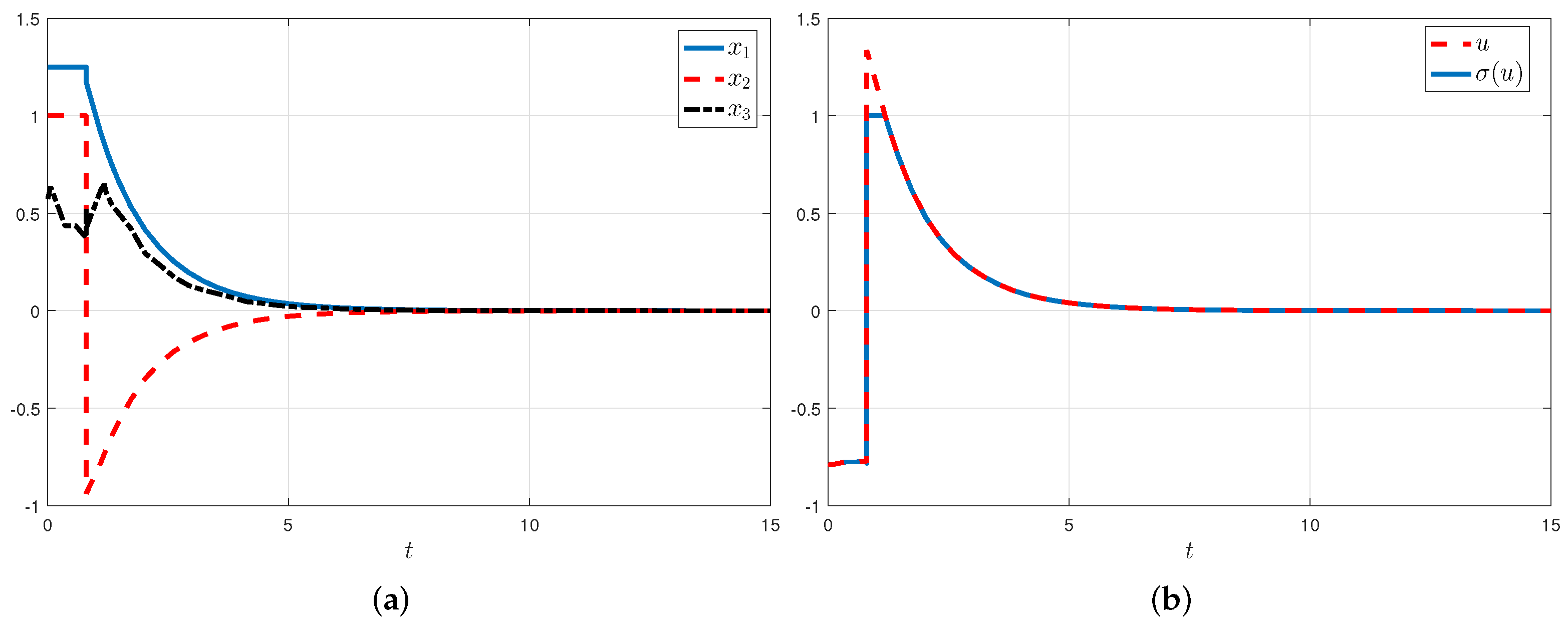
Our goal in this section is to illustrate the effectiveness of the proposed control scheme by comparing it with the relevant work proposed in [45] for an inverted pendulum system described by the interval type-2 fuzzy model without delay and saturation. The following is a system that describes the process:

$$\left\{\begin{array}{c}{\dot{x}}_1\left(t\right)=x_2\left(t\right)\hfill \\ {\dot{x}}_2\left(t\right)=f\left(\mathit{x}\left(t\right)\right)x_1\left(t\right)+h\left(\mathit{x}\left(t\right)\right)u\left(t\right)\hfill \\ 0=Lsin\left(x_1\left(t\right)\right)-x_3\left(t\right)\hfill \end{array}\right.$$

(26)

Non-linear functions $f\left(\mathit{x}\right(t\left)\right)$ and $h\left(\mathit{x}\right(t\left)\right)$ are defined as

$$\begin{array}{cccc}\hfill f\left(\mathit{x}\right(t\left)\right)& =\frac{\left(g-a{m}_{p}L{x}_2^2\left(t\right)cos\left(x_1\left(t\right)\right)\right)sin\left(x_1\left(t\right)\right))}{\left(4L/3-a{m}_{p}L{x}_2^2\left(t\right){cos}^2\left(x_1\left(t\right)\right)\right)x_1\left(t\right)},\hfill & \hfill h\left(\mathit{x}\right(t\left)\right)& =\frac{-acos\left(x_1\left(t\right)\right)}{4L/3-a{m}_{p}L{cos}^2\left(x_1\left(t\right)\right)}\hfill \end{array}$$

$x_1\left(t\right)$ represents the angle between the pendulum and vertical, $x_2\left(t\right)$ represents the angular velocity, and $x_3\left(t\right)$ is the relative horizontal distance between the pendulum center and cart. The force applied to the cart is given by $u\left(t\right)$. The numerical values of the model are: $2L=1$ m is the length of the pendulum, $g=9.8$ m/s² is the gravity acceleration, $m_c\in \left[23\right]$ kg is the mass of the cart, $m_p\in \left[816\right]$ kg is the mass of the pendulum, and $a=1/(m_c+m_p)$. For the sake of this study, the inverted pendulum was taken to operate in a domain fixed by $x_1\left(t\right)\in [-{\displaystyle \frac{5\pi }{12}}{\displaystyle \frac{5\pi }{12}}]$, and $x_2\left(t\right)\in [-55]$.

Next, we describe the inverted pendulum system (26) as follows:

$$\mathit{E}\dot{x}\left(t\right)=\sum _{i=1}^4{\mu }_i\left(\mathit{x}\left(t\right)\right)\left((1-\beta ){\mathit{A}}_i\mathit{x}\left(t\right)\left(t\right)+\beta {\mathit{A}}_i\mathit{x}\left(t\right)(t-d\left(t\right))+{\mathit{B}}_i\mathit{u}\left(t\right)\right)$$

(27)

where $\beta =0.1$, and

$$\begin{array}{cc}\hfill \mathit{E}& =\left[\begin{array}{ccc}1& 0& 0\\ 0& 1& 0\\ 0& 0& 0\end{array}\right],\hspace{1em}{\mathit{A}}_1={\mathit{A}}_2=\left[\begin{array}{ccc}0& 1& 0\\ 0& 0& 0\\ 10.0078& 0& -1\end{array}\right],\hspace{1em}{\mathit{A}}_3={\mathit{A}}_4\left[\begin{array}{ccc}0& 1& 0\\ 0& 0& 0\\ 18.4800& 0& -1\end{array}\right]\hfill \\ \hfill {\mathit{B}}_1& ={\mathit{B}}_3=\left[\begin{array}{c}0\\ 0\\ -0.1765\end{array}\right]{\mathit{B}}_2={\mathit{B}}_4=\left[\begin{array}{c}0\\ 0\\ -0.0206\end{array}\right]\hfill \end{array}$$

Table 4. Lower and upper membership functions of the inverted pendulum.

Lower Membership Functions	Upper Membership Functions
${\underline{\omega }}_{{\mathcal{M}}_1^1}\left(x_1\left(t\right)\right)={\underline{\omega }}_{{\mathcal{M}}_1^2}\left(x_1\left(t\right)\right)=\frac{f_{1max-f_1}}{f_{1max}-f_{1min}}$	${\overline{\omega }}_{{\mathcal{M}}_1^1}\left(x_1\left(t\right)\right)={\overline{\omega }}_{{\mathcal{M}}_1^2}\left(x_1\left(t\right)\right)=\frac{f_{1max-f_1}}{f_{1max}-f_{1min}}$
${\underline{\omega }}_{{\mathcal{M}}_1^3}\left(x_1\left(t\right)\right)={\underline{\omega }}_{{\mathcal{M}}_1^4}\left(x_1\left(t\right)\right)=1-{\underline{\omega }}_{{\mathcal{M}}_1^1}\left(x_1\left(t\right)\right)$	${\overline{\omega }}_{{\mathcal{M}}_1^3}\left(x_1\left(t\right)\right)={\overline{\omega }}_{{\mathcal{M}}_1^4}\left(x_1\left(t\right)\right)=1-{\overline{\omega }}_{{\mathcal{M}}_1^1}\left(x_1\left(t\right)\right)$
with $x_2\left(t\right)=0$, $m_p=m_{pmax}$ and $m_c=m_{cmin}$	with $x_2\left(t\right)=x_{2max}$, $m_p=m_{pmax}$ and $m_c=m_{cmin}$
${\underline{\omega }}_{{\mathcal{M}}_2^1}\left(x_2\left(t\right)\right)={\underline{\omega }}_{{\mathcal{M}}_2^3}\left(x_2\left(t\right)\right)=\frac{f_{2max-f_2}}{f_{2max}-f_{2min}}$	${\overline{\omega }}_{{\mathcal{M}}_2^1}\left(x_2\left(t\right)\right)={\overline{\omega }}_{{\mathcal{M}}_2^3}\left(x_2\left(t\right)\right)=\frac{f_{2max-f_2}}{f_{2max}-f_{2min}}$
${\underline{\omega }}_{{\mathcal{M}}_2^2}\left(x_2\left(t\right)\right)={\underline{\omega }}_{{\mathcal{M}}_2^4}\left(x_2\left(t\right)\right)=1-{\underline{\omega }}_{{\mathcal{M}}_2^1}\left(x_2\left(t\right)\right)$	${\overline{\omega }}_{{\mathcal{M}}_2^2}\left(x_2\left(t\right)\right)={\overline{\omega }}_{{\mathcal{M}}_2^4}\left(x_2\left(t\right)\right)=1-{\overline{\omega }}_{{\mathcal{M}}_2^1}\left(x_2\left(t\right)\right)$
with $m_p=m_{pmin}$ and $m_c=m_{cmax}$	$m_p=m_{pmin}$ and $m_c=m_{cmax}$

defines the lower and upper membership functions used for this example.

We choose the controller membership functions as ${\underline{\nu }}_1\left(x_1\left(t\right)\right)={\overline{\nu }}_1\left(x_1\left(t\right)\right)=0.3e^{(-x_1^2\left(t\right)/0.35)}$, ${\underline{\nu }}_2\left(x_1\left(t\right)\right)={\overline{\nu }}_2\left(x_1\left(t\right)\right)=0.3-{\underline{\nu }}_1\left(x_1\left(t\right)\right)$, ${\underline{\nu }}_3\left(x_1\left(t\right)\right)={\overline{\nu }}_3\left(x_1\left(t\right)\right)=0.7e^{(-x_1^2\left(t\right)/0.35)}$, and ${\underline{\nu }}_4\left(x_1\left(t\right)\right)={\overline{\nu }}_4\left(x_1\left(t\right)\right)=0.7-{\underline{\nu }}_3\left(x_1\left(t\right)\right)$.

Let $d_1=0$, $d_2=0.05$, $\overline{u}=300$, ${\kappa }_1=0.9$, and ${\kappa }_2=0.8$, ${\kappa }_3=0.9$, and ${\kappa }_4=0.8$. Problem (23) produces a feasible solution for ${\lambda }_1=122$ and ${\lambda }_2=122$. The controller gains are listed below.

$$\begin{array}{cc}\hfill & \begin{array}{cc}\hfill {\mathit{H}}_1& =\left[\begin{array}{ccc}485.99& 150.97& 0\end{array}\right],\hfill \\ \hfill {\mathit{K}}_1& =\left[\begin{array}{ccc}7949.1& 2472.3& 338.89\end{array}\right],\hfill & \hfill {\mathit{K}}_2& =\left[\begin{array}{ccc}11109& 3457.4& 469.51\end{array}\right],\hfill \\ \hfill {\mathit{K}}_3& =\left[\begin{array}{ccc}7965.8& 2469.4& 338.69\end{array}\right],\hfill & \hfill {\mathit{K}}_4& =\left[\begin{array}{ccc}11170& 3457.7& 469.7\end{array}\right],\hfill \end{array}\hfill \end{array}$$

(28)

To perform some simulations, based on the parameters mentioned above and the controller in [45] with the following gains:

$$\begin{array}{cc}\hfill & \begin{array}{cccc}\hfill {\mathit{K}}_1& =\left[\begin{array}{ccc}-1174.4396& -189.5425& -96.3306\end{array}\right],\hfill & \hfill {\mathit{K}}_2& =\left[\begin{array}{ccc}-256.0090& 2.4789& -61.9688\end{array}\right]\hfill \end{array}\hfill \end{array}$$

(29)

different cases are considered:

Case 1:

Delay does not affect system. Here, we set $\beta =0$, and both controllers are applied to the system under $\mathbf{\varphi }\left(t\right)={[-{\displaystyle \frac{\pi }{6}},3,0.5]}^{\top }$. The evolution of the state signals is plotted in Figure 3.

Case 2:

A delay affects the system. By using the gains in (28) and (29), respectively, for $\beta =0.1$ and the above delay parameters, the simulation results are shown in Figure 3 and Figure 4 for the initial condition $\mathbf{\varphi }\left(t\right)={[-{\displaystyle \frac{\pi }{20}},0.5,0.5]}^{\top },t\in [-0.050]$.

Case 3:

A delay and saturation affect the system. For this case, Figure 5 shows the states and saturated input signals of the pendulum system when the control law calculated using (28) is implemented for different delays and different initial conditions.

Figure 3 indicates that the two implemented controllers are capable of guaranteeing a convergence of the system’s states when the latter is not affected by delay and saturation. However, in contrast, as can be seen from Figure 4, the controller proposed by [45] is not able to stabilize the system when the delay occurs. Upon examination of the plotted figure in Figure 5, it is evident that the presented control law stabilizes the system despite the time-varying delay and saturation of inputs.

It should be noted that the simulation is conducted assuming measurement errors in $m_p$ and $m_c$, which appear in membership functions such that $m_c=2.5+0.5sin\left(t\right)$ and $m_p=12+4sin\left(t\right)$. This means that the stability conditions based on the type-1 fuzzy system cannot be applied. In light of these results, the synthesized control law is effective in stabilizing the underlying system as well as remaining robust despite input saturation and uncertainty.

4.3. Comparative Explanations

The suggested strategy in this article can effectively solve the problem of admissibilization for mass–spring–damper and inverted pendulum mechanical systems based on the IT-2 fuzzy singular model subject to the time-varying delay and actuator saturation constraints. When compared to previous findings, the following are the primary advantages of the suggested method:

(i)

Compared to existing findings in [22,24,46], the outcome developed in this paper is more realistic and general, since the IT-2 fuzzy model incorporates the system uncertainties. In addition, the premise membership functions of fuzzy controllers and fuzzy systems are not the same.

(ii)

Though further results for interval-valued fuzzy singular systems have been published, such as [36,45], none of these results will be applicable when the system under examination exhibits actuator saturation.

(iii)

For this class of systems, considering the effects of dynamic quantization, using a dynamic/static output feedback controller or an observer-based controller [16] can be a significant issue.

5. Conclusions

An attempt was made in this study to provide solutions to the main challenges that come up when dealing with non-linear singular systems, such as uncertainty, time-varying delay, and saturation. The proposed control scheme emphasizes the use of a state feedback controller based on an IT-2 fuzzy model that exploits both the lower and upper membership functions to adequately characterize uncertainties. By employing an appropriate Lyapunov–Krasovskii functional with convex optimization techniques, the controller existence was analyzed. The proposed control scheme was validated by numerical simulations considering mass–spring–damper and inverted pendulum systems. Research areas that need to be pursued in the near future include quantized output feedback stabilization problems for Markovian jump singular IT-2 fuzzy systems with sensor and actuator saturation.

References

1. Dai, L. Singular Control Systems; Lecture Notes in Control and Information Sciences; Springer: New York, NY, USA, 1989; Volume 118. [Google Scholar]
2. Regaiega, M.A.; Kchaou, M.; Mohamed Chaabane, A.E.H. Robust H guaranteed cost control for discrete-time switched singular systems with time-varying delay. Optim. Control Appl. Meth. 2019, 40, 119–140. [Google Scholar] [CrossRef]
3. Wu, Y.; Lu, R.; Shi, P.; Su, H.; Wu, Z. Analysis and design of synchronization for heterogeneous network. IEEE Trans. Cybern. 2018, 48, 1253–1262. [Google Scholar] [CrossRef] [PubMed]
4. Wu, Y.; Lu, R. Event-based control for network systems via integral quadratic constraints. IEEE Trans. Circuits Syst. Pap. 2018, 65, 1386–1394. [Google Scholar] [CrossRef]
5. Wu, Y.; Lu, R.; Shi, P.; Su, H.; Wu, Z.G. Sampled-Data Synchronization of Complex Networks With Partial Couplings and T-S Fuzzy Nodes. IEEE Trans. Fuzzy Syst. 2018, 26, 782–793. [Google Scholar] [CrossRef]
6. Mahmoud, M. Switched Time-Delay Systems; Springer: Boston, MA, USA, 2010. [Google Scholar]
7. Gu, K.; Kharitonov, V.; Chen, J. Stability of Time-Delay Systems; Springer: Berlin/Heidelberg, Germany, 2003. [Google Scholar]
8. Kchaou, M. Robust observer-based sliding mode control for nonlinear uncertain singular systems with time-varying delay and input non-linearity. Eur. J. Control 2019, 49, 15–25. [Google Scholar] [CrossRef]
9. Feng, Z.; Li, W.; Lam, J. New admissibility analysis for discrete singular systems with time-varying delay. Appl. Math. Comput. 2015, 265, 1058–1066. [Google Scholar] [CrossRef]
10. Wu, Z.; Li, B.; Gao, C.; Jiang, B. Observer-based H control design for singular switching semi-Markovian jump systems with random sensor delays. ISA Trans. 2019, 124, 290–300. [Google Scholar] [CrossRef] [PubMed]
11. Chen, J.; Lin, C.; Chen, B.; Wang, Q. Mixed H and passive control for singular systems with time delay via static output feedback. Appl. Math. Comput. 2017, 293, 244–253. [Google Scholar] [CrossRef]
12. Jiang, B.; Gao, C.; Xie, J. Passivity based sliding mode control of uncertain singular Markovian jump systems with time-varying delay and nonlinear perturbations. Appl. Math. Comput. 2015, 271, 187–200. [Google Scholar] [CrossRef]
13. Zhiqiang, Z.; Daniel, W.H.; Yijingm, W. Fault tolerant control for singular systems with actuator saturation and nonlinear perturbation. Automatica 2010, 46, 569–576. [Google Scholar]
14. Zhang, L.; Boukas, E.K.; Haidar, A. Delay-range-dependent control synthesis for time-delay systems with actuator saturation. Automatica 2008, 44, 2691–2695. [Google Scholar] [CrossRef]
15. Tarbouriech, S.; Gomes da Silva, J. Synthesis of controllers for continuous-time delay systems with saturating controls via LMIs. IEEE Trans. Autom. Control 2000, 45, 105–111. [Google Scholar] [CrossRef] [Green Version]
16. Fu, L.; Ma, Y.; Wang, C. Mix quantized control for singular time-delay system with nonlinearity and actuator saturation. J. Frankl. Inst. 2020, 357, 3953–3974. [Google Scholar] [CrossRef]
17. Xie, X.; Lam, J.; Fan, C.; Wang, X.; Kwok, K.W. Energy-to-Peak Output Tracking Control of Actuator Saturated Periodic Piecewise Time-Varying Systems With Nonlinear Perturbations. IEEE Trans. Syst. Man Cybern. Syst. 2021, 52, 2578–2590. [Google Scholar] [CrossRef]
18. Jemai, W.J.; Jerbi, H.; Abdelkrim, M.N. Nonlinear state feedback design for continuous polynomial systems. Int. J. Control Autom. Syst. 2011, 9, 566–573. [Google Scholar] [CrossRef]
19. Kchaou, M. Robust H Observer-Based Control for a Class of (TS) Fuzzy Descriptor Systems with Time-Varying Delay. Int. J. Fuzzy Syst. 2017, 19, 909–924. [Google Scholar] [CrossRef]
20. Yan, S.; Gu, Z.; Park, J.H.; Xie, X. Sampled Memory-Event-Triggered Fuzzy Load Frequency Control for Wind Power Systems Subject to Outliers and Transmission Delays. IEEE Trans. Cybern. 2022, 1–11. [Google Scholar] [CrossRef]
21. Yan, S.; Gu, Z.; Park, J.H.; Xie, X. Adaptive Memory-Event-Triggered Static Output Control of T-S Fuzzy Wind Turbine Systems. IEEE Trans. Fuzzy Syst. 2022, 30, 3894–3904. [Google Scholar] [CrossRef]
22. Xiaojing, H.; Yuechao, M.; Lei, F. Finite-time dynamic output-feedback dissipative control for singular uncertainty T–S fuzzy systems with actuator saturation and output constraints. J. Frankl. Inst. 2020, 357, 4543–4573. [Google Scholar]
23. Selvaraj, P.; Kaviarasan, B.; Sakthivel, R.; Karimi, H.R. Fault-tolerant SMC for Takagi–Sugeno fuzzy systems with time-varying delay and actuator saturation. IET Control Theory Appl. 2017, 11, 1112–1123. [Google Scholar] [CrossRef]
24. Dang, Q.V.; Vermeiren, L.; Dequidt, A.; Dambrine, M. LMI approach for robust stabilization of Takagi–Sugeno descriptor systems with input saturation. IMA J. Math. Control Inf. 2017, 35, 1103–1114. [Google Scholar] [CrossRef]
25. Yuecha, M.; Menghua, C.; Qingling, Z. Memory dissipative control for singular T–S fuzzy time-varying delay systems under actuator saturation. J. Frankl. Inst. 2015, 352, 3947–3970. [Google Scholar]
26. Mendel, J.M.; John, R.I.; Liu, F. Interval Type-2 Fuzzy Logic Systems Made Simple. IEEE Trans. Fuzzy Syst. 2006, 14, 808–821. [Google Scholar] [CrossRef]
27. Li, Y.; Lam, H.K.; Zhang, L.; Li, H.; Liu, F.; Tsai, S.H. Interval type-2 fuzzy-model-based control design for time-delay systems under imperfect premise matching. In Proceedings of the 2015 IEEE International Conference on Fuzzy Systems (FUZZ-IEEE), Istanbul, Turkey, 2–5 August 2015; pp. 1–6. [Google Scholar] [CrossRef] [Green Version]
28. Jerbi, H.; Kchaou, M.; Alshammari, O.; Abassi, R.; Popescu, D. Observer-based feedback control of interval-valued fuzzy singular system with time-varying delay and stochastic faults. Int. J. Comput. Commun. Control 2022, 17, 3894–3904. [Google Scholar] [CrossRef]
29. Najariyan, M.; Qiu, L. Interval Type-2 Fuzzy Differential Equations and Stability. IEEE Trans. Fuzzy Syst. 2022, 30, 2915–2929. [Google Scholar] [CrossRef]
30. Fu, L.; Lam, H.K.; Liu, F.; Zhou, H.; Zhong, Z. Robust Tracking Control of Interval Type-2 Positive Takagi–Sugeno Fuzzy Systems With External Disturbance. IEEE Trans. Fuzzy Syst. 2022, 30, 4057–4068. [Google Scholar] [CrossRef]
31. Song, W.; Tong, S. Fuzzy decentralized output feedback event-triggered control for interval type-2 fuzzy systems with saturated inputs. Inf. Sci. 2021, 575, 639–653. [Google Scholar] [CrossRef]
32. Li, H.; Pan, Y.; Zhou, Q. Filter Design for Interval Type-2 Fuzzy Systems With D Stability Constraints Under a Unified Frame. IEEE Trans. Fuzzy Syst. 2015, 23, 719–725. [Google Scholar] [CrossRef]
33. Kavikumar, R.; Sakthivel, R.; Kaviarasan, B.; Kwon, O.; Marshal Anthoni, S. Non-fragile control design for interval-valued fuzzy systems against nonlinear actuator faults. Fuzzy Sets Syst. 2019, 365, 40–59. [Google Scholar] [CrossRef]
34. Yan, S.; Gu, Z.; Park, J.H.; Xie, X. Distributed-Delay-Dependent Stabilization for Networked Interval Type-2 Fuzzy Systems With Stochastic Delay and Actuator Saturation. IEEE Trans. Syst. Man Cybern. Syst. 2022, 1–11. [Google Scholar] [CrossRef]
35. Chen, Y.; Fei, S.; Li, Y. Robust Stabilization for Uncertain Saturated Time-Delay Systems: A Distributed-Delay-Dependent Polytopic Approach. IEEE Trans. Autom. Control 2017, 62, 3455–3460. [Google Scholar] [CrossRef]
36. Feng, Z.; Shi, P. Admissibilization of Singular Interval-Valued Fuzzy Systems. IEEE Trans. Fuzzy Syst. 2017, 25, 1765–1776. [Google Scholar] [CrossRef]
37. Park, I.S.; eun Park, C.; Kwon, N.K.; Park, P. Dynamic output-feedback control for singular interval-valued fuzzy systems: Linear matrix inequality approach. Inf. Sci. 2021, 576, 393–406. [Google Scholar] [CrossRef]
38. Zhengchao, X.; Deli, W.; Pak Kin, W.; Wenfeng, L.; Jing, Z. Dynamic-output-feedback based interval type-2 fuzzy control for nonlinear active suspension systems with actuator saturation and delay. Inf. Sci. 2022, 607, 1174–1194. [Google Scholar]
39. Chang, W.-J.; Lin, Y.-W.; Lin, Y.-H.; Pen, C.-L.; Tsai, M.-H. Actuator Saturated Fuzzy Controller Design for Interval Type-2 Takagi-Sugeno Fuzzy Models with Multiplicative Noises. Processes 2021, 9, 823. [Google Scholar] [CrossRef]
40. Gassara, H.; Kchaou, M.; Hajjaji, A.E.; Chaabane, M. Control of Time Delay Fuzzy Descriptor Systems with Actuator Saturation. Circuits Syst. Signal Process. 2014, 33, 3739–3756. [Google Scholar] [CrossRef]
41. Feng, Z.; Zhang, H.; Du, H.; Jiang, Z. Admissibilisation of singular interval type-2 Takagi–Sugeno fuzzy systems with time delay. IET Control Theory Appl. 2020, 14, 1022–1032. [Google Scholar] [CrossRef]
42. Park, P.; Lee, W.I.; Lee, S.Y. Auxiliary function-based integral inequalities for quadratic functions and their applications to time-delay systems. J. Frankl. Inst. 2015, 352, 1378–1396. [Google Scholar] [CrossRef]
43. Uezato, E.; Ikeda, M. Strict LMI conditions for stability, robust stabilization, and H control of descriptor systems. In Proceedings of the IEEE Conference on Decision and Control, Phoenix, AZ, USA, 7–10 December 1999; pp. 4092–4097. [Google Scholar]
44. Sun, X.; Zhang, Q. Admissibility Analysis for Interval Type-2 Fuzzy Descriptor Systems Based on Sliding Mode Control. IEEE Trans. Cybern. 2019, 49, 3032–3040. [Google Scholar] [CrossRef]
45. Sun, X.; Zhang, Q. Admissibility analysis of interval type-2 uncertain stochastic descriptor systems. Neurocomputing 2018, 311, 387–396. [Google Scholar] [CrossRef]
46. Zhu, B.; Zhang, X.; Zhao, Z.; Xing, S.; Huang, W. Delay-Dependent Admissibility Analysis and Dissipative Control for T-S Fuzzy Time-Delay Descriptor Systems Subject to Actuator Saturation. IEEE Access 2019, 7, 159635–159650. [Google Scholar] [CrossRef]
Figure 1. Mass–spring–damper system.
Actuators 12 00030 g001
Figure 2. Simulation plots for mass–spring–damper system. (a) Trajectories of x 1 ( t ) , x 2 ( t ) , and x 3 ( t ) . (b) Ideal and saturated control input signals. (c) Estimated domains of attraction and state trajectories under various initial conditions.
Actuators 12 00030 g002aActuators 12 00030 g002b
Figure 3. State trajectories of the system without delay.
Actuators 12 00030 g003
Figure 4. State trajectories of the system with delay.
Actuators 12 00030 g004
Figure 5. State trajectories using the proposed controller for different delays and initial conditions.
Actuators 12 00030 g005