Abstract
This paper presents a novel approach for analyzing and optimizing motion coupling in the coordinated operation tasks of flexible space multi-arm robots (FMSRs). The method integrates motion coupling between multiple arms and system stiffness to improve the motion and force accuracy of FMSRs by optimizing the configuration. First, a comprehensive model of an FMSR is established using the hypothetical modal method. Then, the motion coupling relationship among multiple arms is analyzed, and a motion coupling degree evaluation index is developed. Furthermore, the constraint relationship of coordinated operation is analyzed, and an equivalent stiffness model for the coordinated operation of the FMSR is formulated along with a stiffness evaluation index. Based on these analyses, the motion trajectory of the FMSR is optimized by comprehensively considering both the motion coupling degree and the equivalent stiffness factors. Finally, numerical simulation experiments are conducted to validate the proposed method, and the results show that the accuracy of the FMSR can be improved by 40% using this approach.
1. Introduction
The coordinated operation of flexible space multi-arm robots (FMSRs) has become increasingly important in the field of robotics due to its wide range of applications [1]. However, the inevitable flexibility of the robot’s links can cause vibrations during motion, resulting in low motion accuracy. In addition, the complex coupling relationship in the motion of FMSRs further reduces the motion accuracy. These problems can lead to changes in the force of the arms and further lead to force unbalance between the arms, causing instability in the FMSR’s control system when performing coordinated tasks. The different ways of improving the motion accuracy of dual/multi-arm robots with rigid links are no longer applicable [2]. Therefore, it is imperative to develop a method that can improve motion accuracy by reducing the vibration amplitude and coupling degree, thereby ensuring successful task execution.
Existing research has mainly focused on developing control strategies and trajectory optimization methods to suppress vibration and improve motion accuracy in manipulators [3]. However, for FMSRs with high coupling and non-linear characteristics, active vibration control parameters are difficult to optimize optimally. In addition, most active vibration control methods require the use of external sensors, and the controller structure is complex and costly. In contrast, the trajectory optimization method determines the objective function by building a dynamic model of the flexible linkage mechanism and then uses a heuristic algorithm to optimize the trajectory that can achieve the lowest vibration and coupling during motion [4,5]. At present, there are three main methods for improving the accuracy of flexible robots through trajectory optimization: reducing the degree of motion coupling, improving stiffness, and energy-based methods.
Liu [6] designed a minimum disturbance controller based on energy conservation to optimize the disturbances generated by the vibration of a dual-arm space robot and improved the tracking accuracy. Cui [5] et al. established an optimal objective function to minimize the residual vibration of a flexible manipulator using joint acceleration constraints and boundary conditions and performed joint trajectory optimization using a conventional PSO algorithm. Zhang [7] established an optimization model for residual vibration and energy consumption considering constraints such as joint stiffness. However, the methods based on energy cannot guarantee the accuracy of the external force while improving the positional accuracy. The accuracy of the force is very important in coordinated operations; otherwise, the controller may become unstable, and its equipment may become damaged.
Numerous researchers have sought ways to improve the stability and accuracy of robots through the stiffness matrix. In one study [8], a multi-objective optimization method based on maneuverability and equivalent stiffness was proposed to obtain optimized operating postures with better equivalent stiffness while avoiding singular conformations and staying away from joint rotation limits. Lin [9] established a spatial distribution mapping of the dexterity performance index, the equivalent stiffness index, and deformation for the end of industrial robots in the whole working space, respectively, and selected the robot end position by equivalent stiffness mapping. Qu [10] used the half-axis length of the equivalent stiffness ellipsoid as an adaptation function and performed pose optimization of a seven-axis redundant manipulator based on a genetic algorithm. Cai [11] obtained an empirical formula for the displacement prediction of vibration intensity by the equivalent stiffness matrix and optimized the attitude based on this empirical formula to obtain a vibration-stabilized machining posture. ABB [12] used the equivalent stiffness model for the real-time compensation of machining deformation. In another study [13], the motion accuracy of the manipulator was improved by establishing and optimizing the stiffness index of the task direction. The authors of [14] sought to find a way to improve the stability and accuracy of the robot system through the force–deformation relationship described by the stiffness matrix. Although the above studies improve the accuracy and stability of the robot, they do not consider the motion coupling characteristics of the system. For FMSRs with strong coupling properties, optimizing only the equivalent stiffness may enhance the degree of motion coupling in certain configurations, particularly the degree of motion coupling between the arms. Thus, such methods suffer from the same problems as the energy-based methods. In addition, these stiffness-based methods are mostly specific to a single manipulator and are not directly applicable to FMSRs, which have complex constraint relationships.
To address the coupling relationship between the manipulator and the base, Yan [15] optimized the motion trajectory of the manipulator by considering the complex factors involved in coupling. Qing [16] et al. proposed a trajectory planning method for a dual-arm space robot that minimizes the disturbance of the base pose caused by motion coupling. In [17], a rigid–flexible hybrid dual-arm coordinated path planning method based on maneuverability optimization was proposed. Several studies [15,16,17] concern the problem of accuracy caused by motion coupling between robots and the base or the operated object. Numerous researchers have investigated the motion coupling of manipulators. Shum [18] described the magnitude of the perturbation caused by the manipulator’s motion to the base and introduced the concept of the coupling factor to investigate the velocity coupling between the manipulator and the base. Xu [19] developed a new dynamic coupling model for free-floating space manipulators, which overcame the challenge of measuring the coupling characteristics. According to the conservation of momentum equation, Zhou [20] obtained a speed relationship matrix between the space manipulator base and the joint or capture target and proposed the dynamic coupling coefficient and coupling ellipse to measure the degree of coupling. In other studies in the literature [18,19,20], the kinematic coupling between the base and joint end of a space manipulator has been investigated, and evaluation metrics such as coupling factors and coupling coefficients have been developed. Deshan [21,22] established a coupling model between a flexible base and a manipulator and defined a metric to quantify the degree of motion coupling between the flexible base and the manipulator. Xu [23] constructed a vibration minimum objective function based on the relationship between joint motion and the vibration of the flexible body. Du [24] derived a dynamic coupling matrix for a flexible space manipulator and used a multi-pulse robust input shaper to suppress the vibration of the flexible structure. The above studies have only analyzed the motion coupling of a single manipulator, but the motion coupling between multiple arms caused by vibrations is not yet clear. Therefore, these results cannot be directly applied to the coordinated operation of FMSRs.
Considering the advantages of the above three methods, we decided to use motion coupling combined with the stiffness method to improve the motion accuracy of FMSRs. However, the above studies also have the following problems: ① The methods based on energy or stiffness cannot guarantee the accuracy of the external force while improving the positional accuracy, which is very limited in coordinated operations. ② The motion coupling between multiple arms caused by vibrations is not yet clear. ③ Due to the complicated constraints involved in the coordinated operation of FMSRs, the existing research on rigid–flexible motion coupling and the stiffness analysis of manipulators cannot be directly applied to FMSRs.
This paper proposes a novel method for analyzing and optimizing motion coupling in the coordinated operation of FMSRs. In Section 2, we construct an FMSR model. In Section 3, we analyze the inter-arm motion coupling relationship and design an evaluation index for the coupling degree. In Section 4, we develop an equivalent stiffness model for the FMSR and analyze the constraint relationship involved in its coordinated operation and then design a stiffness evaluation index. In Section 5, by integrating the motion coupling degree and equivalent stiffness, we optimize the motion trajectory of the FMSR. In the last section, a simulation test demonstrates the effectiveness of our method in significantly improving the motion accuracy of the coordinated operation of FMSRs.
2. FMSR Modeling
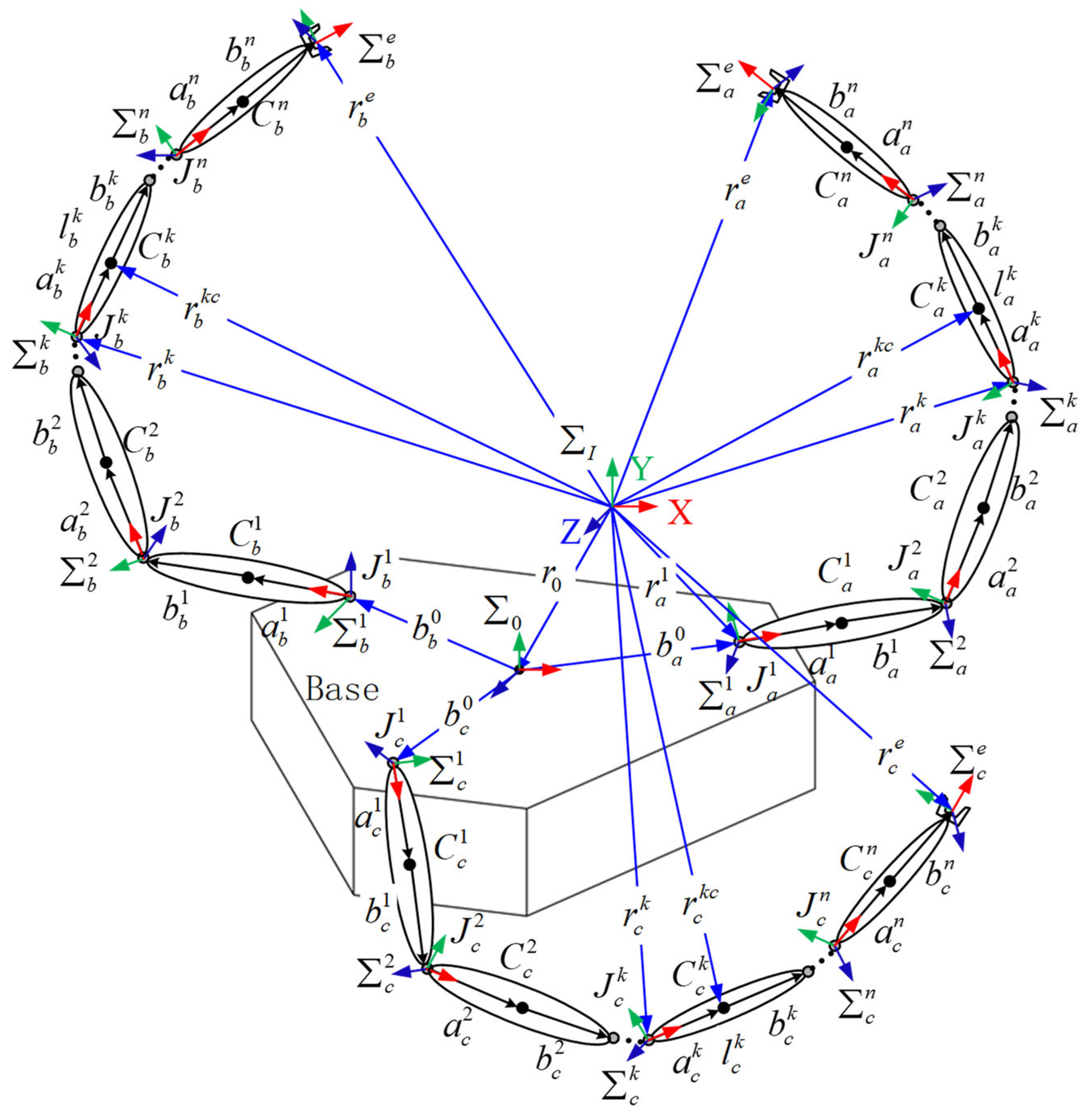
Let an FMSR have arms (), where the joint degree of freedom of the arm () is . A three-arm robot is shown in Figure 1.
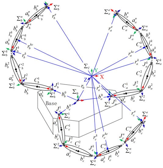
Figure 1.
Schematic diagram of a three-arm robot.
The symbols in Figure 1 are defined as follows:
The inertial coordinate frame;
The centroid coordinate frame of the base;
The end coordinate frame of arm ();
The coordinate frame of link of arm ();
The degrees of freedom of arm ;
The centroid of link of arm ;
The joint between links and of arm ;
The length of link of arm ;
The vector connecting to ;
The vector connecting to ;
The vector from the centroid of the base to the first joint of arm ;
The position vector of the base centroid;
The end position vector of arm ;
The position vector of ;
The position vector of link ’s centroid of arm .
2.1. Coordinate Transformation of Flexible Link
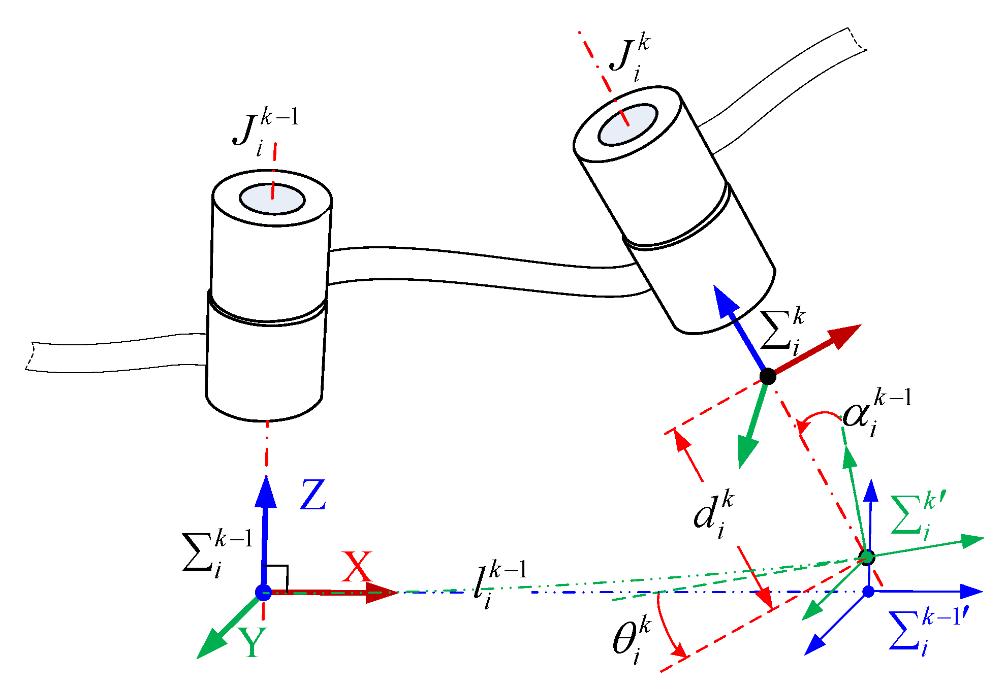
A flexible link is considered a continuous elastic structure. The floating frame of reference formulation is used to describe the deformation of the flexible link in this paper. We use the link of arm , shown in Figure 1, as an example for specific analysis and establish its coordinate frame according to the modified Denavit–Hartenberg (MDH) method, as shown in Figure 2. and are the first and last coordinate frames of link , respectively. Let there be two coordinate frames, and , at the end of the link to describe the posture before and after the link deformation. For a rigid link, the attitude of both coordinate frames coincides with .
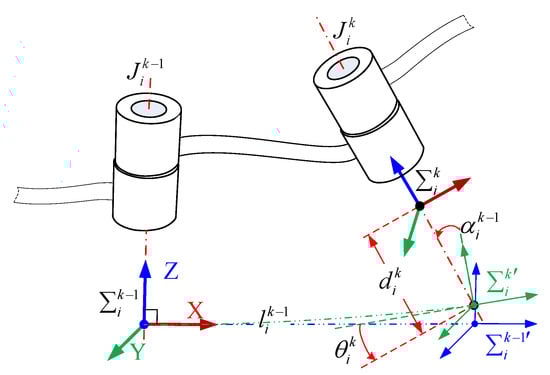
Figure 2.
Diagram of the coordinate frame of the flexible link of arm .
For defining the transformation that transforms the vectors defined in to their description in , the transformation matrix can be written as
where denotes the transformation matrix that translates along the X-axis, denotes the transformation matrix that rotates around the X-axis, and so on [25]. , , , and denote the parameters of MDH. denotes the transformation matrix of the flexible deformation, and its expression is given in the literature [26].
where denotes the sum of the first orders of vibrations of arm ’s link , is the -th order vibration modal function of arm ’s link , is the component of the -th order modal coordinate of link along the -axis, and so on. Since the longitudinal and torsional vibrations of the flexible link are generally neglected, it is known that , .
2.2. Kinematic Model
Considering the flexibility factor, we extend the mathematical model in [27] to FMSRs. Let denote the transformation matrix of the base coordinate frame with respect to the inertial frame . According to Equation (1), the link transformations can be multiplied together to find the single transformation that relates frame to frame :
The angular velocity of the -th link’s centroid and the angular velocity of the end under the inertia frame are as follows:
where denotes the attitude angular velocity of the base spacecraft. is the unit vector along the frame Z-axis described in . is the rotation matrix that relates frame to frame , and its expression can be obtained from Equation (4). is the angular velocity of link ’s centroid relative to the frame, is the angular velocity of the end of link relative to the frame, specified as follows:
where is a function of the Euler angles, which represents the mapping matrix from the Euler angles’ speed to the angular velocity. Since the vibration characteristics of the flexible link in this paper exhibit low amplitude and high frequency, can be considered as the identity matrix. In this paper, symbols are defined in the coordinate frame indicated by their left superscript, and symbols without a left superscript indicate the description in the inertial frame.
The centroid linear velocity of link and the linear velocity of the end under the inertia frame are expressed as follows:
where denotes the linear velocity of the base spacecraft centroid, , and . is the linear velocity of link ’s centroid relative to the frame; specifically,
Using Equations (6) and (8), a new equation is derived as follows:
where denotes the differential vector of the base pose; denotes the joint angle of arm ; , , and . is the Y-axis component of the -th order modal coordinates of arm ’s link . denotes the base-arm Jacobi; denotes the joint-arm Jacobi; and denotes the modal-arm Jacobi.
The mapping relationship between the end velocity of the flexible three-arm space robots and the base velocity, the joint angular velocity, and the modal velocity can be obtained as follows:
where ,,,, , .
3. Motion Coupling Analysis of the FMSR
3.1. Kinematic Decoupling
In the case where the position and attitude of the base of the FMSR are free, it is necessary to decouple the kinematic equations using the momentum conservation law. In this section, the momentum equations of the FMSR are derived.
The linear momentum of the FMSR can be expressed as the sum of the linear momentum of each link.
where is the mass of the base, and is the mass of arm ’s link . is the number of arms.
The angular momentum of the FMSR can be expressed as follows:
where denotes the angular momentum of the FMSR with respect to the base centroid, written as
where and denotes the base inertia and link inertia, respectively.
By combining the linear and angular momentum given in Equations (11) and (12), respectively, the momentum equation for the FMSR can be derived as follows:
where , , and is given in Appendix A.
When the position and attitude of the base are free, the linear and angular momentums of the FMSR are both equal to zero, denoted as . Based on this, the momentum conservation equation of the FMSR in the floating base mode can be derived as follows:
where and . Since the initial momentum of the FMSR in the floating base mode is zero, we can obtain the velocity mapping relationship between the modal coordinates and the base, and the velocity mapping relationship between the modal coordinates and joint angles.
where and are functions of , , and .
Substituting Equation (16) into Equation (10), we obtain the mapping relationship between and , which can be expressed as follows:
where is the Jacobi matrix of the modal coordinates and the end velocity. is denoted in chunks as follows:
3.2. Degree of Motion Coupling
The diagonal elements in Equation (18) represent the mapping relationship between the modal velocity of each robotic arm and its corresponding end velocity. The off-diagonal elements of the matrix represent the mapping relationship between the modal velocity of an arm through the base to the end velocity of another arm, which is referred to as the inter-arm modal motion coupling relationship.
To characterize the influence of modal velocity on the end velocity of the FMSR, metrics for the degree of modal velocity coupling must be defined. Various mathematical metrics have been proposed by scholars to quantitatively evaluate the degree of the singularity of Jacobi matrices. In this paper, the operability degree is chosen as the comprehensive index to evaluate the degree of modal velocity coupling, which can reflect the overall influence of modal coordinates on the velocity of the FMSR. The operability values of , of , and of are used to evaluate the degree of two-by-two coupling of the three-arm end velocity caused by the modal velocity.
4. Equivalent Stiffness Analysis of Coordinated Operating System for the FMSR
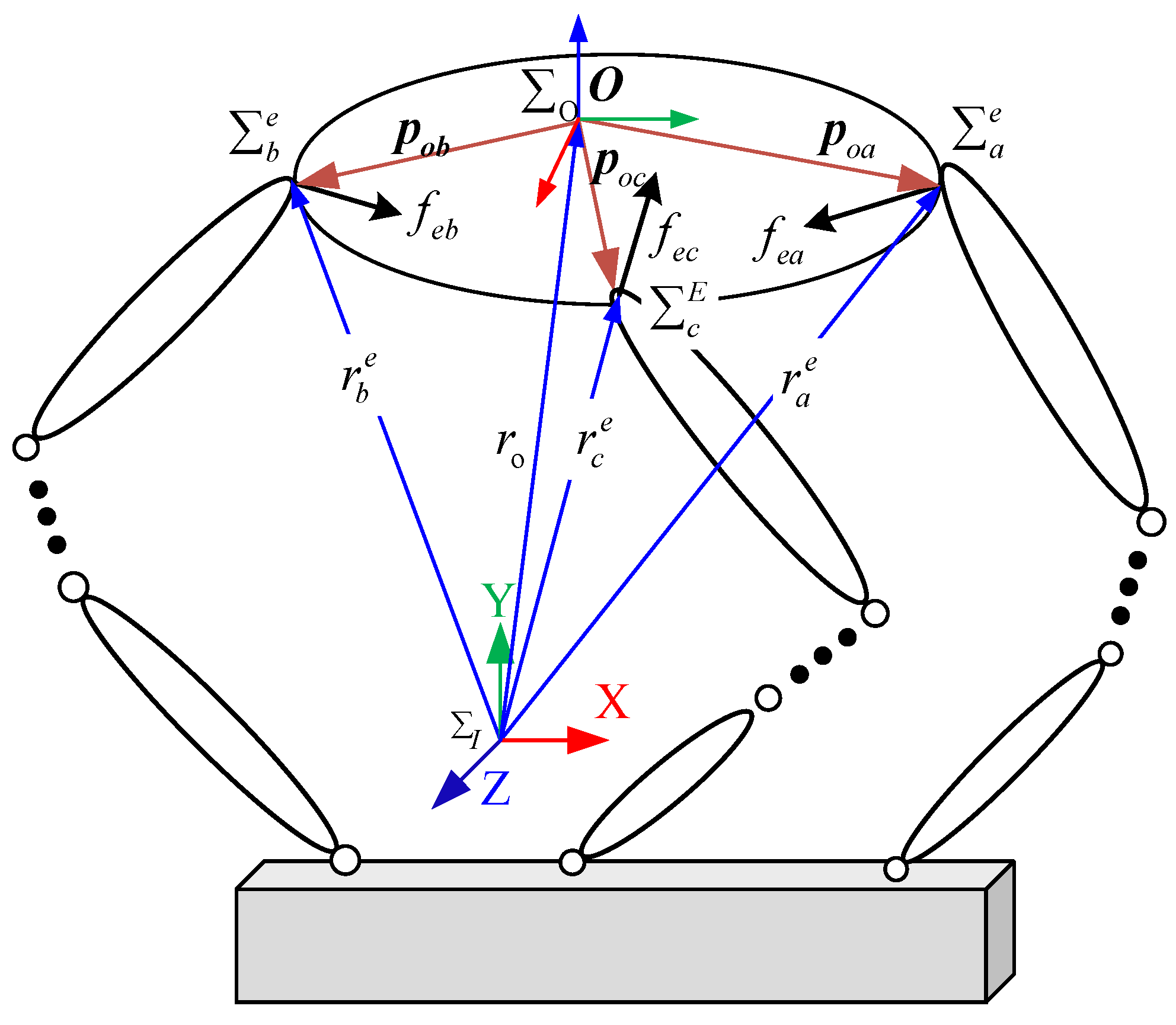
Figure 3 illustrates the coordinated operation system of an FMSR with a rigid body, which is subject to the following assumptions:
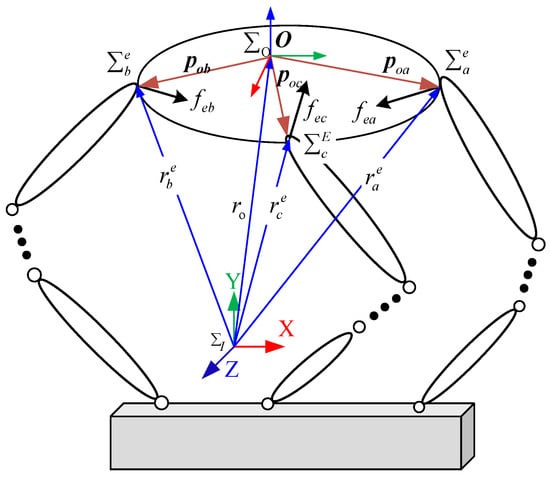
Figure 3.
The coordinated operation of an FMSR with a rigid body.
- ➢
- The end gripper of each robot arm and the rigid body are in a state of no relative displacement;
- ➢
- The entire coordinated operating system of the FMSR is in static equilibrium;
- ➢
- The positional deformation generated in the system satisfies the small deformation condition.
The rigid body coordinate frame is established with the centroid of the rigid body as the origin. The grasping coordinate frame is established with the grasping point at the end of the arm as the origin. It is assumed that the rigid body has infinite stiffness and does not deform under the action of the output force at the end of the robot arm and the external environmental force. To establish the virtual grasping coordinate frame , frame is translated to the origin of as the virtual grasping point.
The solution of the stiffness matrix of the flexible manipulator is given in the literature [13]. The total deformation at frame is the sum of the deformation generated by joint flexibility, linkage flexibility, and the servo.
where the flexibility matrix of the manipulator represents the linear relationship between the external force applied to the end and the resulting deformation caused by the force. The equivalent stiffness matrix of the manipulator end can be represented by the inverse matrix of the flexibility matrix .
4.1. Motion Constraint Relationship
In the inertia frame , the frame , the frame , and the frame can be mathematically represented as follows:
where the position vector is represented by ,, and respectively. Since the axes’ orientation of the frame coincides with that of , the attitude angle is represented by and , respectively.
Assuming a sufficiently large stiffness of the body and negligible deformation under external forces, the origin of frames and will always coincide. Therefore, the pose constraints between the body and the virtual grasping point can be expressed as follows:
4.2. Force Constraint Relationship
In the frame, the output force of the FMSR can be represented as follows:
where and are the output force and torque at the end of each arm, is the position vector from the centroid of the rigid body to the end of each arm, is the grasping matrix of the arm, and denotes the antisymmetric matrix of .
The total external forces acting on the body can be expressed as follows:
where is the grasping matrix of the FMSR, and denotes the end output force of the FMSR.
4.3. Coordinated Operating System Equivalent Stiffness Model
Applying the principle of virtual work, the total work performed by the force can be expressed as follows:
and satisfy Hooke’s law.
where denotes the positional deformation produced by the force; denotes the equivalent flexibility matrix of the multi-arm robot system at the origin ; and , denotes the flexibility matrix of each robot arm in frame .
Rectifying Equations (23), (25) and (26) yields
Then, the equivalent stiffness matrix of the coordinated operating system of the FMSR can be expressed as follows:
Equation (28) characterizes the stiffness performance of the coordinated operating system at the frame . is a 6 × 6 matrix, where each element represents the linear relationship between force and position deformation, as well as moment and angular deformation, resulting in different dimensions. Therefore, to facilitate the analysis, the matrix is divided into four 3 × 3 submatrices.
where denotes position stiffness; denotes attitude stiffness; and and denote position–attitude coupling stiffness.
4.4. Equivalent Stiffness Evaluation Index
Assume that the output of the unit force by the coordination operating system satisfies Equation (30).
Applying the definition of stiffness, Equation (30) can be reformulated as an expression for the stiffness matrix in terms of deformation, given by
Due to the symmetry and positive definiteness of the stiffness matrix, can be decomposed into using singular value decomposition yields, where is a matrix composed of eigenvectors, and is a diagonal matrix composed of singular values , , and . Thus, Equation (31) can be expanded as follows:
Assuming that , , and are substituted and expanded in Equation (32), the following ellipsoidal equation can be obtained:
Equation (33) represents the equivalent flexibility ellipsoid equation, where the half-axis lengths of the three principal axes are the reciprocal of the singular values of the stiffness matrix , and the principal axis direction coincides with the corresponding eigenvectors of the stiffness matrix, respectively. The vector pointing from the origin of the ellipsoid to any point on the surface of the ellipsoid satisfies Equation (30), which represents the flexibility of the coordinated operating system along . The larger the modulus of , the weaker the ability to output force in that direction, and vice versa. Therefore, the shortest half-axis of the flexibility ellipsoid indicates the best stiffness performance of the coordinated operating system.
When operating in interaction with the environment, the FMSR establishes a constraint coordinate frame with the contact point as the origin, and the Z-axis of the constraint coordinate frame is aligned with the normal direction of the constraint surface. In this context, the stiffness model of the system is established at the constraint coordinate frame, and let be the vector along the Z-axis of the constraint coordinate frame that satisfies Equation (30). This vector is defined as the task direction flexibility, which is the deformation produced by the output unit force in the task direction. A smaller value of indicates a better stiffness of the FMSR operating system in the task direction.
5. Motion Accuracy Optimization Method for Coordinated Tasks
5.1. Modeling Multi-Objective Optimization Problems
- Decision variables
The objective of this paper is to optimize the degree of motion coupling and the end equivalent stiffness of the FMSR to achieve optimal performance within its workspace. For a multi-arm robot with three seven-degree-of-freedom redundant manipulators, the decision variables to be optimized are as follows:
- Objective function
In this study, the coordination operation task is used as an example of optimization analysis, and the objective function can be formulated as follows:
Although the multi-objective particle swarm optimization method can obtain the optimal Pareto solution for the multi-objective problem expressed in Equation (36), selecting a suitable solution that meets the task requirements from multiple non-inferior solutions is a new issue. One approach to solving this problem is to obtain the weight coefficients, which can reflect the weight relationship among the indicators by using the covariance matrix. By transforming the multi-objective problem into a single-objective problem using these weight coefficients, the task requirements can be satisfied.
First, it should be noted that the metrics used in the study are dimensionless. Specifically, for the path planning task of the FMSR, a set of indicator values can be obtained for each control cycle during task execution, corresponding to each of the indicators , and . The mean value of each set can then be calculated as follows:
Then, the covariance of the two indicators and can be expressed as follows:
where the denominator uses instead of , which is known as an unbiased estimation. This approach allows for a better estimation of the covariance with a smaller sample. This method can be used to calculate the covariance between any two indicators. The resulting covariance matrix of multiple indicators can be expressed as follows:
The diagonalization of the covariance matrix presented in Equation (39) allows for the decoupling of the coupling relationship between the indicators. Since the covariance matrix is symmetric, there exists an orthogonal matrix that satisfies the relation , where is the diagonalized matrix, and represents the eigenvector matrix of the covariance matrix . The eigenvector matrix can be used to transform the multi-objective optimization problem into a single-objective optimization problem.
Up to now, in solving the covariance matrix of each indicator of the robot, the dimensionless nature of each indicator has been realized. By diagonalizing the covariance matrix, the eigenvector matrix of the covariance matrix can be obtained, which enables the decoupling of each indicator and transforms the multi-objective problem into a single-objective problem.
- Binding conditions
Since the kinematic constraints of the robot were duly considered in the path planning stage, and the motion trajectory of the rigid body was obtained, we now consider the optimization problem using only boundary constraints. These boundary constraints include limits on the velocity and angle that the robot must maintain.
5.2. Solution of Particle Swarm Optimization Algorithm Based on Stochastic Inertia Factor
In this study, the optimization problem presented in Equation (40) is solved using a particle swarm algorithm. Let us denote the position and velocity of the -th particle at step as and respectively. Similarly, let and represent the individual historical optimal solution and the population historical optimal solution of the -th particle at step . The velocity and position update equations can be obtained as follows:
where refers to the inertia factor, controls the dependence of the particle on its initial velocity, and affects its ability to explore the global solution space. The cognitive factor and the random number , which is distributed on the interval , together determine the degree of dependence of the particle on its individual historical optimal solution. The social factor and the random number , also distributed on the interval , together determine the degree of dependence of the particle on the population’s optimal solution.
In this study, a random inertia factor satisfying the normal distribution is used for the PSO algorithm, which tends to oscillate near the global optimal solution in the late stage of the algorithm. The expression for the random inertia factor is as follows:
where and represent the maximum and minimum values of the mean of the random inertia factor, respectively. represents the variance of the random inertia factor. Random number obeys standard normal distribution, and is a random number between 0 and 1.
In this study, the optimization of the robot configuration is performed in the zero space of each arm. Specifically, the vector is mapped to the null space of the arm, and based on this, the velocity and position update equations of the particle swarm are obtained as follows:
where denotes the identity matrix, and is a constraint factor characterizing the degree of particle succession to the speed of the current step update. The values of the above parameters can be adjusted according to the specific requirements of the optimization problem.
The optimization process in this paper involves continuously updating the particle velocity and position using Equation (43). The algorithm terminates when the velocity of each particle becomes 0, and the position no longer changes, or when the maximum number of iterations is reached.
6. Test and Discussion
6.1. Subject
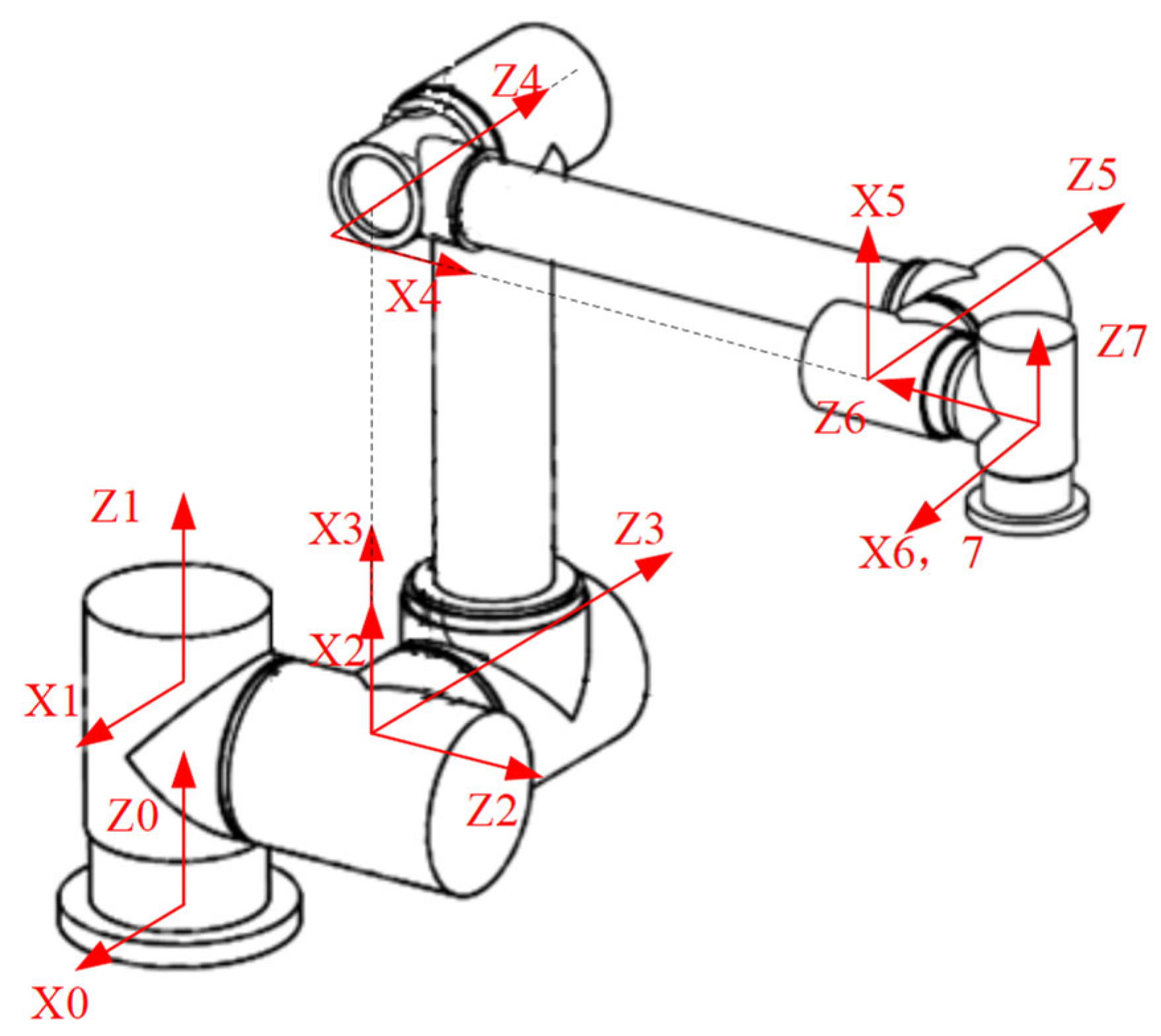
We carried out simulation experiments using a three-arm robot. The three modular arms are named , all of which were configured with a “shoulder3-elbow1-wrist3” structure and had seven degrees of freedom. The shoulder and wrist joints were symmetrical with respect to the elbow joint. The material of the links was aluminum alloy, with an elasticity modulus of 70 GPa. The diameters of link 3 and link 4 were 96 mm and 70 mm, respectively, and the wall thickness was 5 mm. The frame of the arm was established using the MDH method, as shown in Figure 4. The kinematic and dynamic parameters are shown in Table 1 and Table 2, respectively. The initial poses of the three arms in the base frame were [0.5, 0.3, 0, 0, 0, 0], [−0.5, 0.3, 0, 0, 0, 0], and [0, −0.6, 0, 0, 0, 0], respectively. The base mass and inertia were and , respectively.
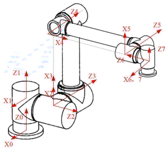
Figure 4.
MDH coordinate frame.

Table 1.
Kinematic parameters.
Table 2.
Dynamics parameters.
6.2. Model Validation
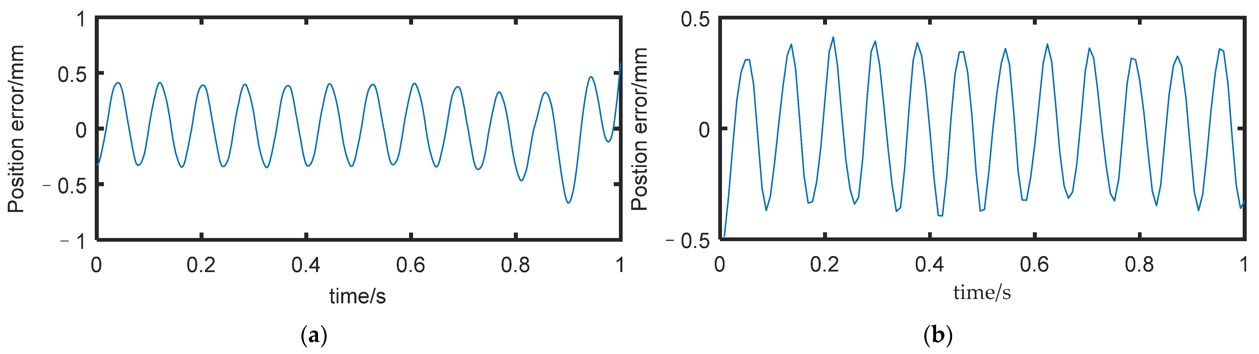
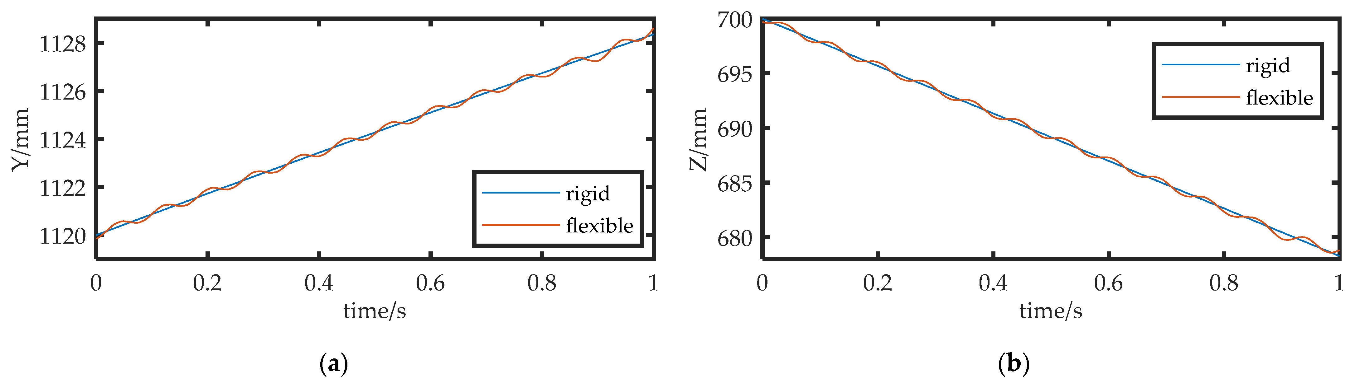
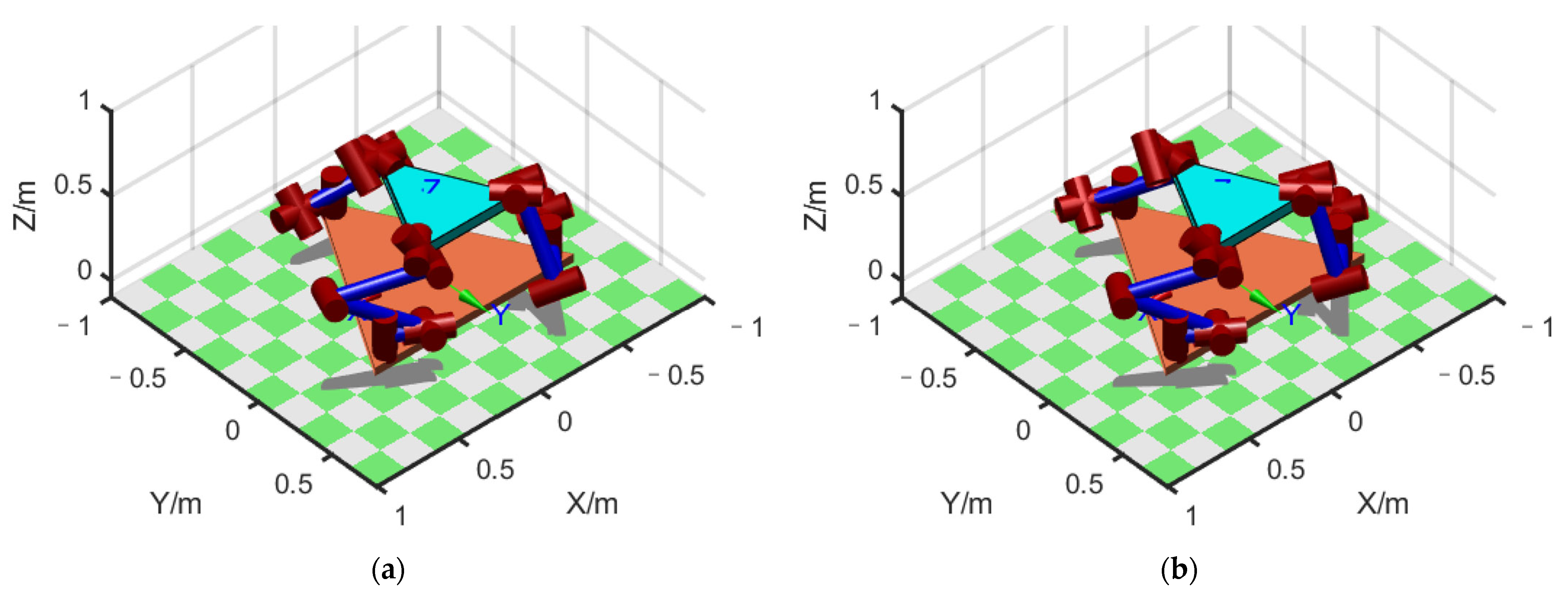
Following the second and third sections, we built a simulation model of the FMSR on a computer using MATLAB and Robotics Toolbox (Peter Corke Release 10), as shown in Figure 5a. ODE45 (Runge–Kutta fourth and fifth order) was used to solve the kinetic differential equations. Although the vibration modes of each link had many orders, the higher order mode had less influence on the amplitude. We intercepted the first three modes to improve computational efficiency. Since the motion of joints 3 and 4 contributed the most to the trajectory error, we set the angular velocity of joints 3 and 4 to 1°/s to obtain the end trajectory. Additionally, we compared it with the trajectory of a rigid arm under the same conditions. The configuration of each arm at the beginning of the model validation experiment was . The position error is shown in Figure 6a. Due to the consistent parameters and configurations of each arm, only the position error of arm a is given here. Figure 7 shows the position and time relationship of arm a during the experiment. As there was no motion or vibration along the X-axis, only the Y-axis and Z-axis results are shown here. It can be seen that the robot continues to vibrate slightly along these two axes, which affects the precision of the trajectory.
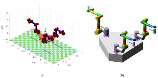
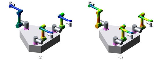
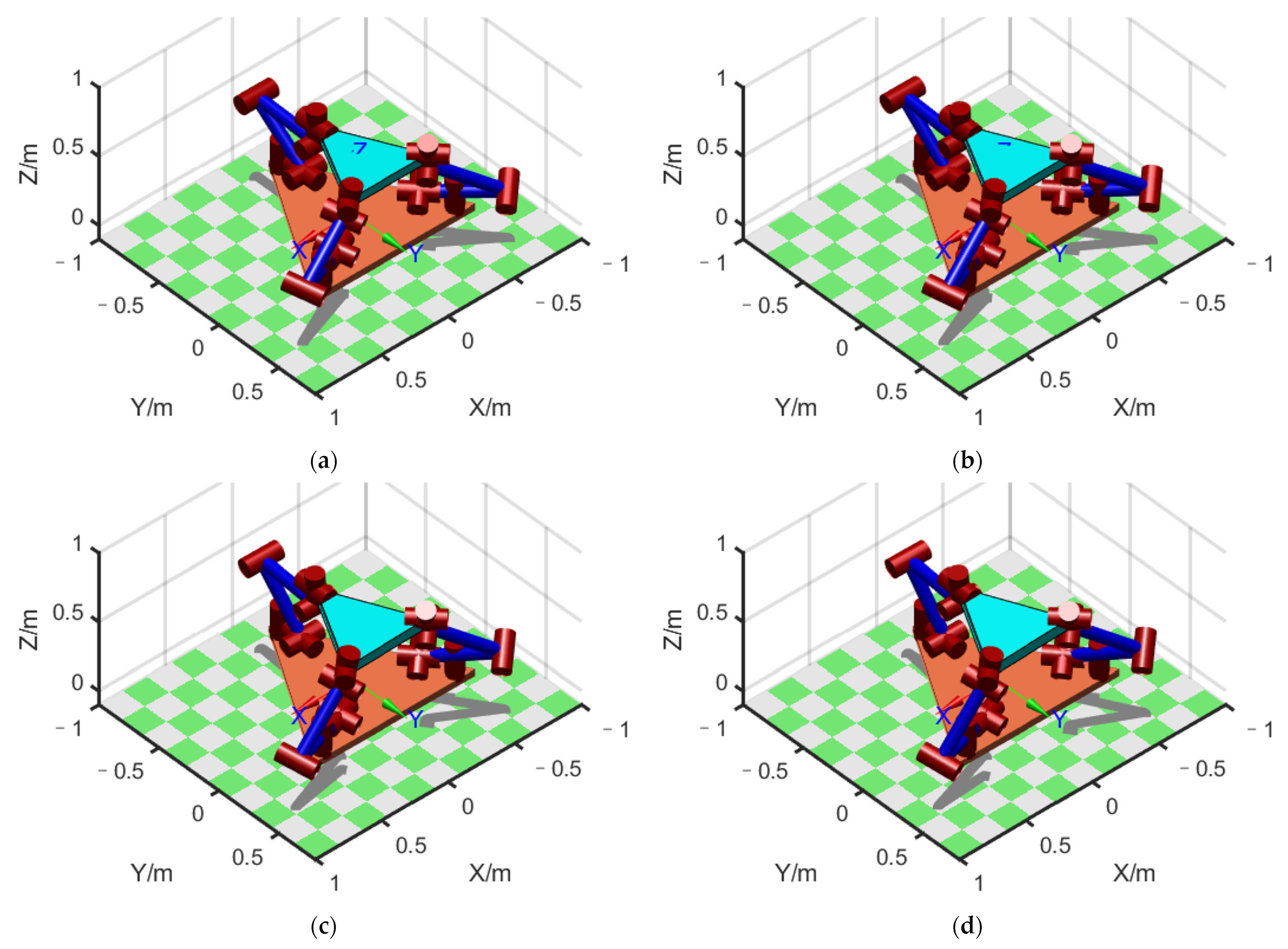
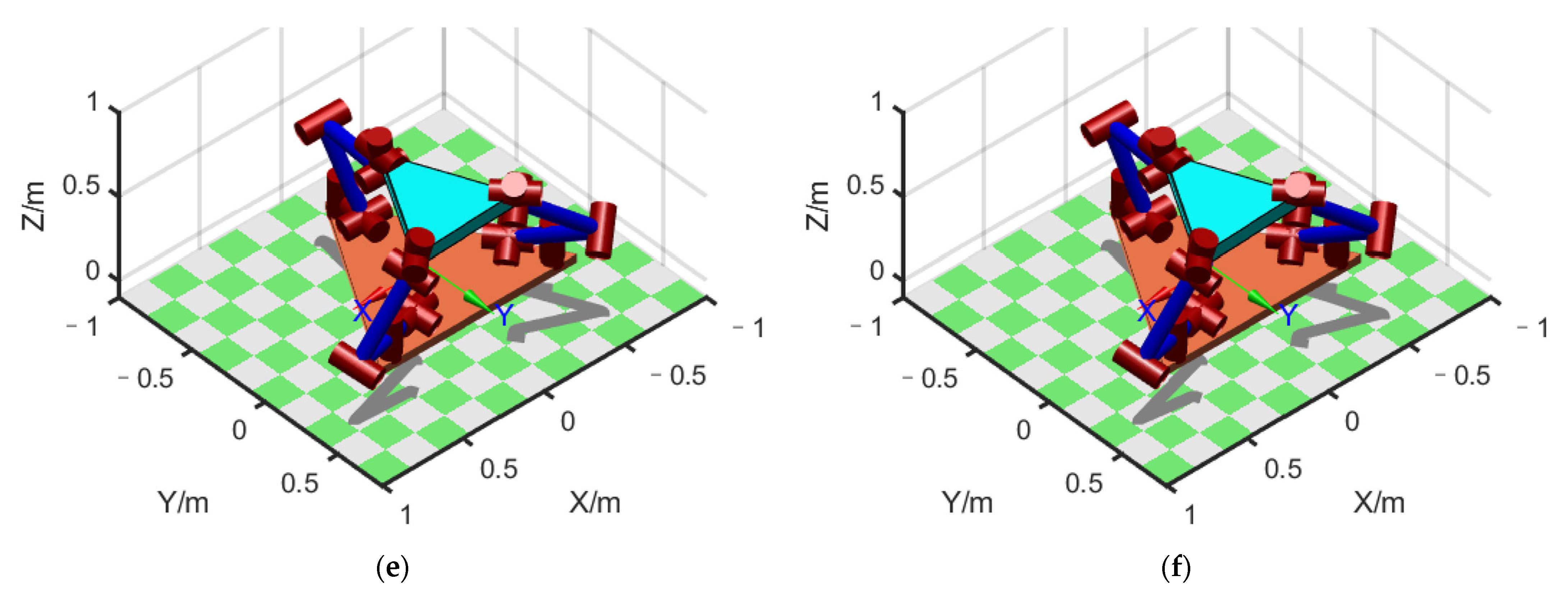
Figure 5.
FMSR model: (a) the model built using MATLAB; (b–d) the configuration changes in the simulation process using ADAMS.
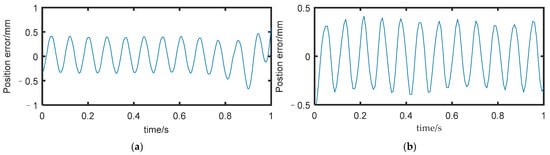
Figure 6.
Position error: (a) the position error obtained using MATLAB; (b) the position error obtained using ADAMS.
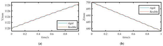
Figure 7.
Position error: (a) position error along Y-axis; (b) position error along Z-axis.
To verify the correctness of the results, a co-simulation environment with MSC/ADAMS and MATLAB/SIMULINK was generated; the 3D model of the FMSR was established in ADAMS, and all control algorithms were generated in SIMULINK. The communication interval between ADAMS and SIMULINK was 0.01, and the simulation mode was set to discrete. To obtain the dynamic response of the flexible links, each link was preprocessed using ABQUS, including mesh partitioning, creating analysis steps (intercepting the first 15th mode), setting boundary conditions, etc., to finally obtain the mnf (modal neutral file). The mnf was then used to replace the rigid links in ADAMS, as shown in Figure 5b–d. Similarly, joints 3 and 4 of each arm were moved at an angular velocity of 1°/s to obtain the position error of the flexible arm and the rigid arm, as shown in Figure 6b. As the arterial angular velocity was relatively small, and the simulation lasted 1 s, the configuration shown in Figure 5b–d does not change significantly. However, the changes in the color of the links show that the joints were constantly moving.
Comparing Figure 6a,b, it can be seen that the model established in this paper and the simulation results using MATLAB are basically consistent with the results of ADAMS in terms of vibration frequency and amplitude, which indicates that the model established in this paper is accurate and effective. However, we were unable to obtain the responses of each vibration mode from ADAMS, and there were also difficulties in simulating over-constrained models, such as coordinated tasks. Therefore, in subsequent analysis, we only used MATLAB for simulation.
6.3. Optimization and Analysis
The robot’s rigid body had a mass of 5 kg, and its cross-sectional shape was a waist triangle with a side length of 0.67 m, 0.67 m, and 0.6 m. The three arms of the FMSR hold the three vertexes of the rigid body and move it from the initial pose to the final pose along the straight-line path, where = [0, 0, 0.6, 0, 0, 0] and = [0.1, 0.1, 0.8, 0, 0, 0]. Let the desired external force of the FMSR be a zero vector. The desired trajectory of the rigid body is obtained using trapezoidal interpolation with the parabolic transition. The motion trajectory of the three arms is derived from the motion constraint relationship. The motion trajectory of each joint is obtained using inverse kinematics.
- Experiment 1
We considered the four points that divided the straight-line path into five equal parts, together with the two endpoints of the path, for a total of six points. We then plotted the configuration diagram separately at these six points to display the changing process of the configuration on the path, as shown in Figure 8a–f. The initial configuration, shown in Figure 8a, was = [114.5°, 11.7°, −78.5°, 56.3°, −63.5°, 160°, −12.5° ], = [−136.8°, −20.0°, −83.2°, 53.7°, −61.0°, 178.4°, −70°], and = [180°, 0°, −143.0°, 55.4°, −2.4°, 0°, 90°].
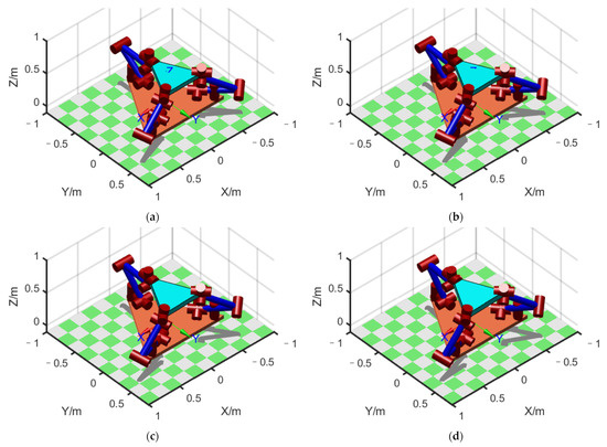

Figure 8.
Configuration of FMSR before optimization: (a–f) configuration at 6 points in sequence.
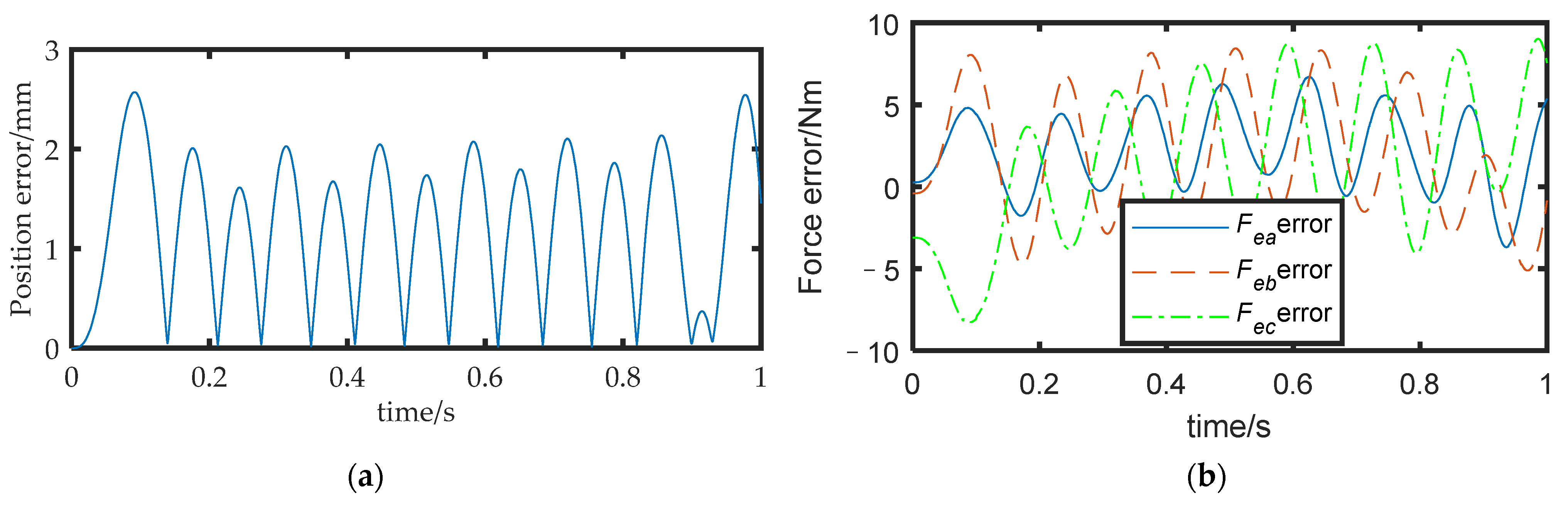
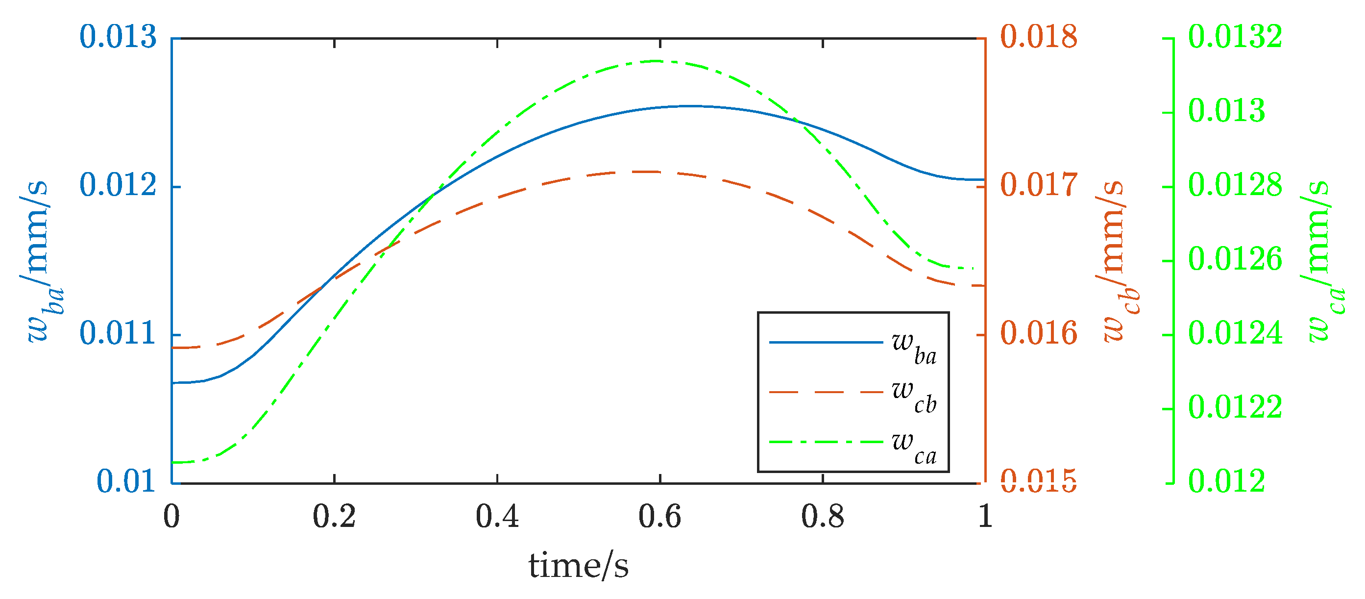
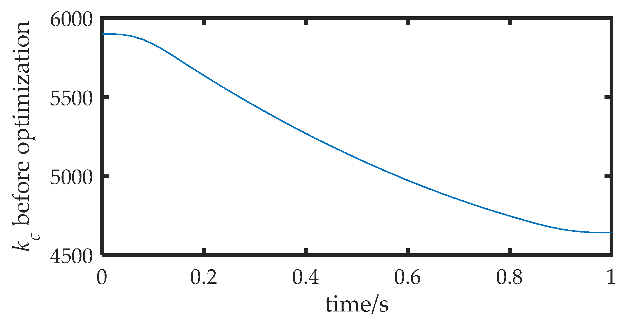
The joint angle was substituted into the model developed in Section 2 to obtain the pose of the FMSR, and the actual trajectory of the rigid body was solved according to the motion and force constraints and compared with the desired trajectory. The position error is shown in Figure 9a, with a maximum value of approximately 2.5 mm. The actual external force of the three arms was obtained according to Equation (20) and compared with the desired external force. The force error is shown in Figure 9b, with a maximum value of approximately 10 N. It can be seen that the position errors due to vibration in coordinated operation and the interaction of the three arms with the rigid body lead to external force errors. Excessive force errors in coordinated operations are dangerous and can easily lead to controller instability. Equation (19) was used to calculate the inter-arm modal motion coupling metrics, as shown in Figure 10. It can be seen that there is motion coupling between the different arms, which means that the movements of the arms affect each other. Equation (34) was used to calculate the task directional stiffness, as shown in Figure 11. It can be seen that when the coupling degree and the directional stiffness are large, the force error is also larger. Therefore, in this study, the accuracy of the FMSR was optimized by establishing the objective function of the coupling degree and the directional stiffness.
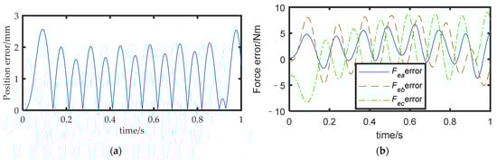
Figure 9.
(a) Position error before optimization; (b) force error before optimization.
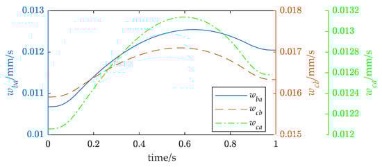
Figure 10.
Inter-arm modal motion coupling metrics before optimization.
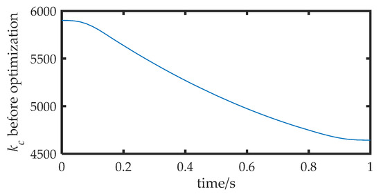
Figure 11.
Task directional stiffness before optimization.
- 2.
- Experiment 2
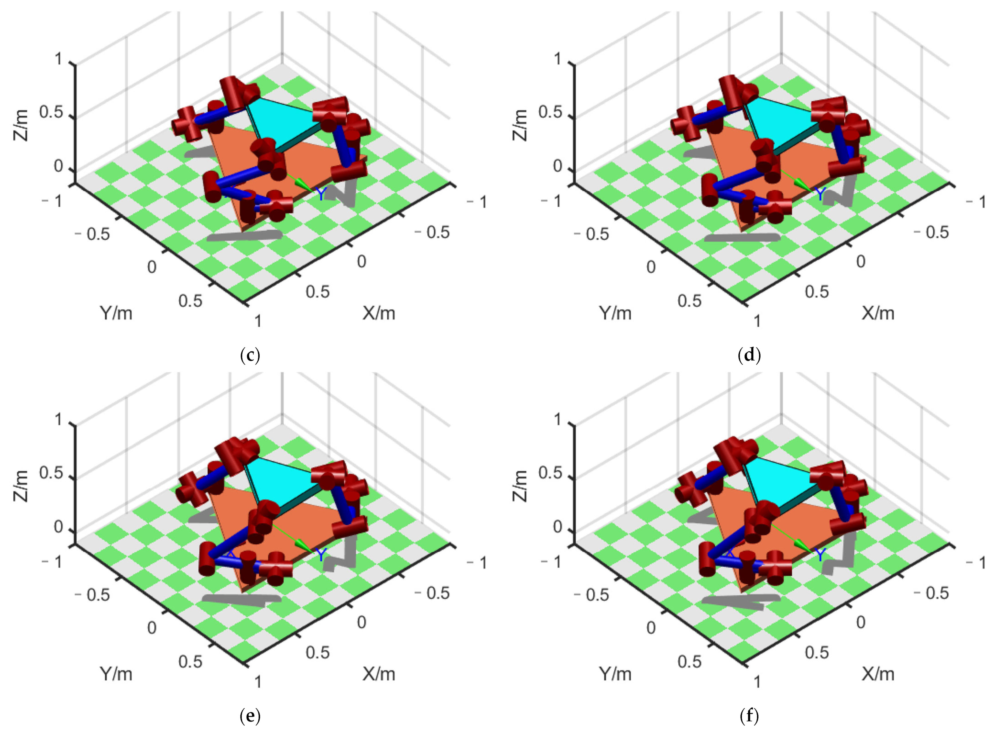
We sought to use the method proposed in this paper to reduce the position error. Using the method developed in Section 5, a model of optimization problems was generated using MATLAB. The number of the particle population was 50, and the maximum iteration was 100 times. The inertia factor was , , and the constraint factor . Equations (41)–(43) were used to optimize each configuration on the expected path. The results of the configuration optimization are shown in Figure 12. The optimized initial configuration was = [62°, −13.2°, −62.7°, 52.9°, −116.7°, 111.4°, 38.5°], = [−216.4°, −21.9°, −92.3°, 38°, −103.6°, 113.4°, −20.5°], and = [85.4°, −36.9°, −159.8°, 26.5°, −54.4°, −53.1°, 186.1°].
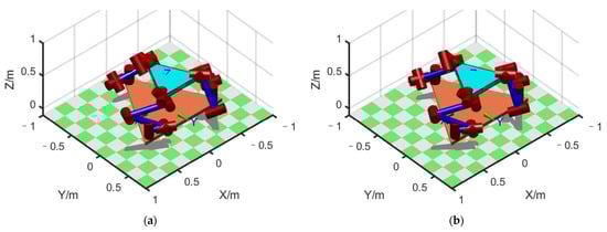
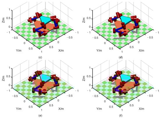
Figure 12.
Configuration of FMSR after optimization: (a–f) configuration at 6 points in sequence.
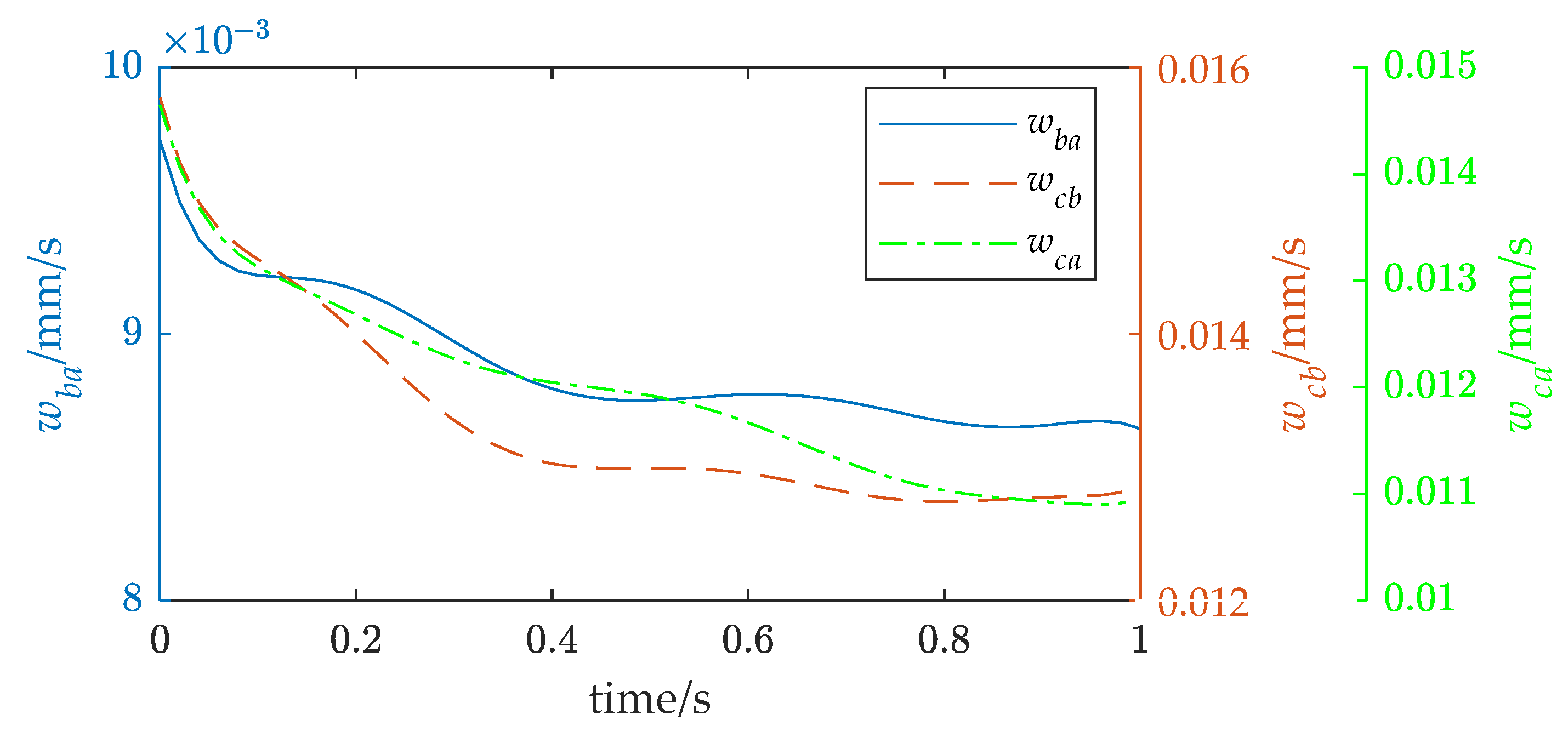
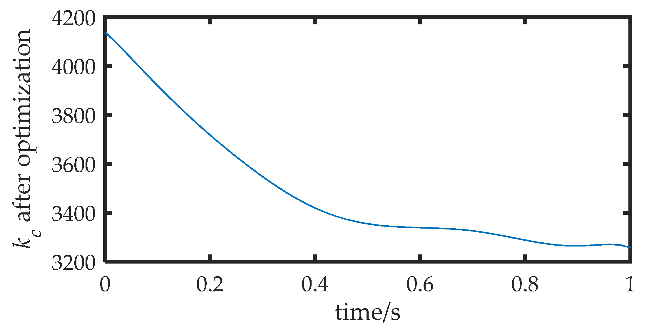
The inter-arm modal motion coupling indices after optimization using the proposed method are shown in Figure 13. Compared with Figure 10, it can be observed that the inter-arm modal motion coupling indices caused by the modal motion were reduced by 15~30% after the optimization. This means that the amplitude of the vibration was reduced, and the degree of motion coupling between the three arms was reduced by up to 30%. The directional flexibility after optimization is shown in Figure 14. A comparison with Figure 11 indicates that the system flexibility in the direction of motion was reduced by 32%.
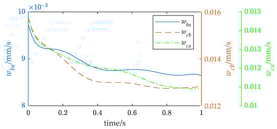
Figure 13.
Inter-arm modal motion coupling metrics after optimization.

Figure 14.
Task directional stiffness after optimization.
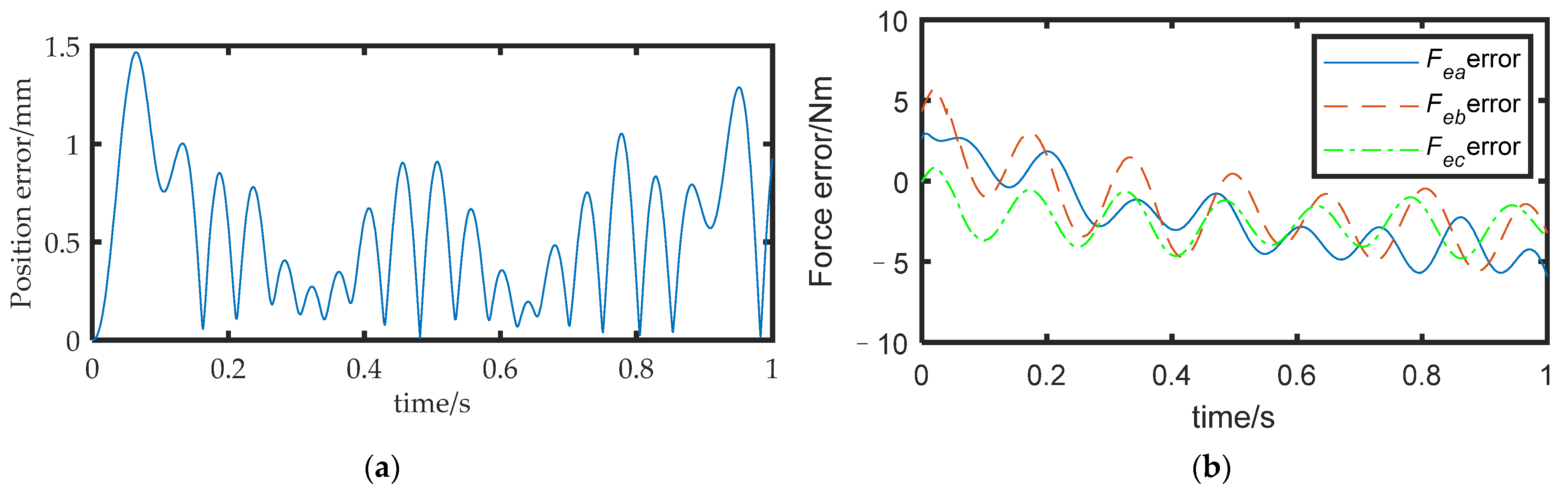
Figure 15a shows the position error between the actual path of the rigid body and the desired path. The results show that the maximum position error before optimization was 2.5 mm (as shown in Figure 9), while the maximum error after optimization was 1.5 mm. The force error is shown in Figure 15b, with a maximum value of approximately 6 N, Comparing Experiments 1 and 2, it can be inferred that the method proposed in this paper could effectively improve the motion accuracy of the FMSR by 40% and improve the accuracy of the external force of the arms.
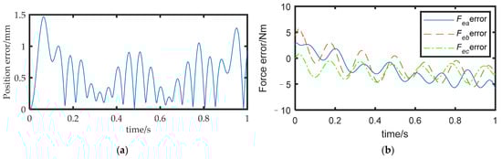
Figure 15.
(a) Position error after optimization; (b) force error after optimization.
A comparison between the experiments without and with the method proposed in this paper is shown in Table 3. It can be seen that the method proposed in this paper could effectively reduce the position error and force error by 40%. The results of the simulation experiment show that the method of this paper is effective in improving the accuracy of the FMSR.
Table 3.
The comparison between the experiments.
7. Conclusions
This paper presents a motion coupling analysis and optimization method to improve motion accuracy in the coordinated operation tasks of FMSRs. The contributions of this study are significant in several aspects. First, a general model of an FMSR was established using the hypothetical modal method. Second, we investigated the rigid–flexible motion coupling law of the FMSR and designed an evaluation index of the coupling degree. Third, the stiffness model of the flexible manipulator was extended to the FMSR by analyzing the constraint relationship in coordinated operation tasks. Finally, we considered the rigid–flexible motion coupling between multiple arms and the stiffness index when optimizing the motion trajectory. This optimization effectively improves the robot’s motion accuracy and force accuracy. Future research will focus on exploring the motion coupling characteristics of the flexible base and the robot during on-orbit assembly tasks and studying the coordination control method under the coupled vibration of the FMSR.
Author Contributions
Conceptualization, G.P., Q.J. and G.C.; software and validation, G.P.; formal analysis, G.P.; resources, Y.W. and G.C.; writing—original draft preparation, G.P.; writing—review and editing, G.P. and F.S.; visualization, G.P. and F.S.; supervision, G.C. All authors have read and agreed to the published version of the manuscript.
Funding
This study was co-supported by the National Natural Science Foundation of China (No. 51975059 and No. 62103058).
Institutional Review Board Statement
Not applicable.
Informed Consent Statement
Not applicable.
Data Availability Statement
Not applicable.
Acknowledgments
The authors would like to acknowledge Huang Zeyuan, Fei Junting, and the Key Laboratory of Space Robotics, Ministry of Education, for their help and expertise.
Conflicts of Interest
The authors declare no conflict of interest.
Appendix A
Substituting Equation (7) into Equation (11) yields
where is the total mass of the system. denotes identity matrix. , is the vector of the system centroid. denotes the antisymmetric matrix of ., , . The expression for , , and is given in Appendix B.
Substituting Equations (5) and (7) into Equation (13) yields
where , , , and ., , and is given in Appendix B.
By substituting Equation (A2) into Equation (12) and combining it with Equation (A1), the expression of , , and are obtained.
Appendix B
The -th columns of the four Jacobi matrix , , , and are , ,, ; columns are , , , ; columns to are all . Both and are unit vectors along the frame axes.
References
- Gan, Y.H.; Dai, X.Z. Survey of coordinated multiple manipulators control. Control Decis. 2013, 28, 321–333. [Google Scholar]
- Qi, W.; Huasong, M.; Yixuan, G. An algorithm for trajectory optimization of dual-arm coordination based on arm angle constraints. Cobot 2022, 1, 10. [Google Scholar]
- Liu, Z.; Sun, R.; Li, M. Research on Trajectory Tracking and Vibration Suppression of a Smart Flexible-joint-and-link Space Manipulator. J. Phys. Conf. Ser. 2019, 1187, 32076. [Google Scholar] [CrossRef]
- Korayem, H.M.; Nikoobin, A.; Azimirad, V. Trajectory optimization of flexible link manipulators in point-to-point motion. Robotica 2009, 27, 825–840. [Google Scholar] [CrossRef]
- Leilei, C.; Hesheng, W.; Weidong, C. Trajectory planning of a spatial flexible manipulator for vibration suppression. Robot. Auton. Syst. 2019, 123, 103316. [Google Scholar]
- Liu, Q.; Shi, S.; Jin, M.; Fan, S.; Liu, H. Minimum disturbance control based on synchronous and adaptive acceleration planning of dual-arm space robot to capture a rotating target. Ind. Robot. 2022, 49, 1116–1132. [Google Scholar] [CrossRef]
- Zhang, H.; Sun, Z.; Fu, Y. Vibration characteristics of flexible manipulator based on EVO trajectory effect by the constraints and parameters variation. J. Vibroeng. 2022, 24, 501–520. [Google Scholar] [CrossRef]
- Jiao, J.; Liao, W.; Tian, W.; Zhang, L.; Liu, S. A configuration optimizing method in robotic machining. Int. Rob. Auto. J. 2017, 3, 287–288. [Google Scholar]
- Lin, Y.; Zhao, H.; Ding, H. Posture optimization methodology of 6R industrial robots for machining using performance evaluation indexes. Robot. Comput. Integr. Manuf. 2017, 48, 59–72. [Google Scholar] [CrossRef]
- Qu, W.; Hou, P.; Yang, G. Research on the stiffness performance for robot machining systems. Acta Aeronaut. Astronaut. Sin. 2013, 31, 2823–2832. [Google Scholar]
- Cai, D.; Ji, S.; Zhang, H. Vibration analysis and prediction of pneumatic wheel in finishing process. China Mech. Eng. 2015, 26, 3082–3086. [Google Scholar]
- Zhang, H.; Wang, J.; Zhang, G.; Gan, Z.; Pan, Z.; Cui, H.; Zhu, Z. Machining with flexible manipulator: Toward improving robotic machining performance. In Proceedings of the 2005 IEEE/ASME International Conference on Advanced Intelligent Mechatronics, Monterey, CA, USA, 24–28 July 2005; IEEE: New York, NY, USA, 2005; pp. 1127–1132. [Google Scholar]
- Pan, G.; Jia, Q.; Chen, G.; Li, T.; Liu, C. A Control Method of Space Manipulator for Peg-in-Hole Assembly Task Considering Equivalent Stiffness Optimization. Aerospace 2021, 8, 310. [Google Scholar] [CrossRef]
- He, J.; Yue, X.; Li, Y. Establishment of Hysteresis Stiffness Model and Kinematic Precision Analysis of Manipulators. J. Mech. Transm. 2022, 46, 21–26. [Google Scholar]
- Lei, Y.; Han, Y.; Wenfu, X.; Zhonghua, H.; Bin, L. Kinodynamic Trajectory Optimization of Dual-Arm Space Robot for Stabilizing a Tumbling Target. Int. J. Aerosp. Eng. 2022, 2022, 9626569. [Google Scholar]
- Qing, Z.; Xiaofeng, L.; Guoping, C. Base attitude disturbance minimizing trajectory planning for a dual-arm space robot. Proc. Inst. Mech. Eng. Part. G. J. Aerosp. Eng. 2022, 236, 704–721. [Google Scholar]
- Hu, Z.; Xu, W.; Yang, T. Coordinated Grasp and Operation Planning for Hybrid Rigid-flexible Dual-arm Space Robot. J. Astronaut. 2022, 43, 1311–1321. [Google Scholar]
- Xu, Y.; Shum, H.Y. Dynamic control and coupling of a free-flying space robot system. J. Field Robot. 2010, 11, 573–589. [Google Scholar] [CrossRef]
- Xu, W.; Peng, J.; Liang, B.; Mu, Z. Hybrid modeling and analysis method for dynamic coupling of space robots. IEEE Trans. Aerosp. Electron. Syst. 2016, 52, 85–98. [Google Scholar] [CrossRef]
- Zhou, Y.; Luo, J.; Wang, M. Dynamic coupling analysis of multi-arm space robot. Acta Astronaut. 2019, 160, 583–593. [Google Scholar] [CrossRef]
- Meng, D.; Liang, B.; Xu, W.; Zhang, B.; Liu, H. Dynamic coupling of space robots with flexible appendages. IEEE Int. Conf. Robot. Biomim. 2016, 2016, 1530–1535. [Google Scholar]
- Meng, D.; Wang, X.; Xu, W.; Liang, B. Space robots with flexible appendages: Dynamic modeling, coupling measurement, and vibration suppression. J. Sound. Vib. 2017, 396, 30–50. [Google Scholar] [CrossRef]
- Xu, W.; Xu, C.; Meng, D. Trajectory planning of vibration suppression for rigid-flexible hybrid manipulator based on PSO algorithm. Control Decis. 2014, 29, 632–638. [Google Scholar]
- Du, Y. Dynamic Coupling and Control of Flexible Space Robots. Int. J. Struct. Stab. Dyn. 2020, 20, 2050103. [Google Scholar] [CrossRef]
- Craig, J.J. Introduction to Robotics: Mechanics and Control; Pearson/Prentice Hall: Upper Saddle River, NJ, USA, 2005. [Google Scholar]
- Jia, Q.; Hong, X.; Chen, G. Vibration analysis of a free-floating flexible space manipulator in on-orbit capture collision. J. Vib. Shock. 2018, 37, 187–195. [Google Scholar]
- Liu, H. Coordinated Motion Planning Study of Dual-Arm Space Robot for Capturing Spinning Target. Ph.D. Thesis, Harbin Institute of Technology, Harbin, China, 2014. [Google Scholar]


Disclaimer/Publisher’s Note: The statements, opinions and data contained in all publications are solely those of the individual author(s) and contributor(s) and not of MDPI and/or the editor(s). MDPI and/or the editor(s) disclaim responsibility for any injury to people or property resulting from any ideas, methods, instructions or products referred to in the content. |
© 2023 by the authors. Licensee MDPI, Basel, Switzerland. This article is an open access article distributed under the terms and conditions of the Creative Commons Attribution (CC BY) license (https://creativecommons.org/licenses/by/4.0/).