1. Introduction
In recent years, absolute pressure measurement technology has become one of the important symbols to measure the degree of industrial technology development of a country and is also an important evaluation indicator of industrial safety [
1,
2,
3]. As an international standard pressure measurement instrument with high accuracy and stability, the absolute pressure piston manometer is based on the hydrostatic equilibrium principle and Pascal’s law for pressure measurement. As the working medium is a gas, the adiabatic manometer is subject to many nonlinear and time-varying factors, which results in relatively long stabilization times and unsatisfactory stability performance. Therefore, it is crucial to design a high-quality control system to address these issues.
Relatively few scholars at home and abroad have studied piston manometer balancing control methods, but for quadrotors [
4,
5], inverted pendulums [
6,
7,
8], balancing vehicles [
9,
10], permanent-magnet synchronous motors [
11,
12], and other such similar balancing systems, there are many modern control algorithms currently applied, such as proportional-integral-derivative (PID) control [
13,
14,
15], linear quadratic regulator control (LQR) [
16,
17], robust control [
18,
19], fuzzy control [
20,
21,
22,
23], adaptive control [
24,
25], sliding mode control [
26,
27,
28], etc. Theoretically, the control methods applied to these equilibrium systems can also be applied to piston manometers. The authors in [
29] introduced the relaxation factor into model predictive control (MPC), on which it was combined with hybrid PID control theory for applied control to improve the control performance of smart car path tracking across the board. The authors in [
30] proposed a Udwadia–Kalaba theory-based adaptive robust control (UKBARC), applied to a permanent-magnet linear synchronous motor, which can both transform the control task with the desired trajectory as the desired constraint and deal effectively with system uncertainty. The authors in [
31] proposed a sliding mode control method incorporating an adaptive strategy to achieve altitude tracking of a quadrotor under strong external disturbances, but the method requires high accuracy of the model and a relatively complex controller structure. The authors in [
32] proposed an improved fuzzy logic controller based on Lyapunov’s criterion for the real-time oscillation and stability control of a coupled two-arm inverted pendulum, which improved the transient and steady-state response speed of the system to a certain extent, but the amount of operations in this controller is large and more difficult to implement in practical engineering. The authors in [
33] combined the quantum particle swarm algorithm (QPSO) with the LQR control method. It used the former to search for the optimal values of the Q matrix as well as the weighting coefficients in the controller, improving the overall control performance of the balancing vehicle, but the time for the algorithm to perform the optimal search still needs to be improved.
Active disturbance rejection control (ADRC) is an “observation + compensation” nonlinear control method proposed by Professor Jingqing Han et al. [
34] to preserve the advantages of PID and overcome its shortcomings. However, the internal parameters are too many, and the rectification process is tedious. Gao [
35] then introduced the concepts of linearization and bandwidth based on the advantages of active disturbance suppression techniques and proposed linear active disturbance rejection control (LADRC) for the first time, making the controller parameters more intuitive and simpler to rectify. In addition, to further improve the control performance of LADRC, many researchers have made further improvements. An improved third-order LADRC controller was proposed by the authors in [
36], introducing the total disturbance differential signal in the LESO and applying a series of first-order inertial links, which improves the system’s ability to suppress high-frequency noise. The authors in [
37] combined robust sliding mode control (SMC) theory with LADRC control to overcome the bandwidth limitation of LADRC itself and improve the control accuracy for the system. The authors in [
38] proposed an improved linear active disturbance suppression control (MLADC) method to compensate the system model into a linear state observer (LESO) to improve its observation accuracy, reduce its state error and enhance the robustness of the system.
However, it is easy to see that most improvements have a common limitation, namely that the controller parameters can only be adjusted manually by trial and error, which is complex and time-consuming, and the fixed parameters also lead to a less robust system, which cannot be applied to specific practical engineering problems. As a nonlinear system, absolute pressure piston manometers cannot be modeled with absolute accuracy. Moreover, when implementing control, uncertainties within the system and external disturbances are inevitable, which can reduce the efficiency of the system [
39], and the stability performance of the system needs to be improved. Fuzzy control is considered to be a control scheme to improve the robustness and adaptability of the system and has been widely used in industry. It can dynamically adjust the parameters of the controller according to the output of the system, thus enabling the controller to track the input signal faster. Therefore, to improve the anti-disturbance capability of the controlled system and make it achieve equilibrium quickly and stably, this paper proposes a FLADRC-based equilibrium control strategy for the adiabatic piston manometer, which introduces the idea of fuzzy control for adaptive parameter adjustment based on LADRC. The feasibility and effectiveness of the control scheme are verified by simulations in MATLAB.
The other sections of the article are organized as follows: In
Section 2, the theoretical modeling of the adiabatic piston manometer is presented. In
Section 3, the specific design and stability analysis of the FLADRC controller is carried out for the controlled system model. In
Section 4, the simulation results of the four control schemes, FLADRC, LADRC, PID, and Kp, are compared and analyzed to verify the performance advantages of the proposed control scheme. Finally, the summary of the research work in this paper is discussed in
Section 5.
2. Theoretical Modeling of an Absolute Pressure Piston Manometer
2.1. The Working Principle of the Absolute Pressure Piston Manometer
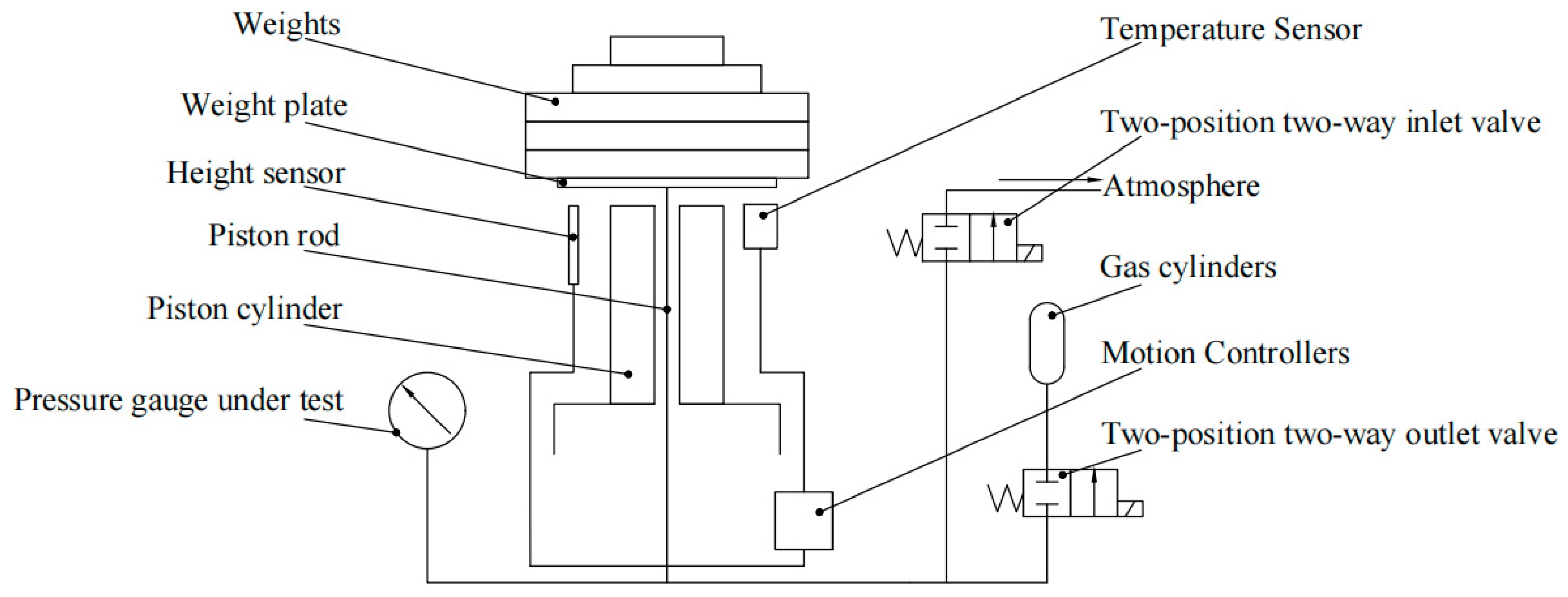
The mechanical structure of the absolute pressure piston manometer as a nonlinear time-varying system is shown in
Figure 1. Before the system starts to work, the corresponding weights are automatically configured according to the measured pressure. The pure gas in the cylinder, which is the working medium for pressurizing the system, is first added quickly to the originally vacuumed piston cylinder through the inlet valve until the weights and the piston is jacked up. Immediately afterward, the piston is subjected to constant changes in height due to the pressure in the piston cylinder and other uncertainties. The gas flow from the inlet and outlet valves is then adjusted in turn according to the actual situation so that the piston is finally stabilized at the preset height. At this point, the weights and piston are then mechanically balanced as a whole, thus completing the measurement and calibration of the pressure.
Based on the above working principle, it can be seen that the most important part of the system is the piston, followed by the electromagnetic switching valve. Therefore, to build a theoretical model for an absolute pressure piston manometer, it is necessary to start with these two parts and carry out the corresponding characteristic analysis.
2.2. Kinetic Analysis of the Weight Combination Section
Throughout the actual working of the system, the weight, the weight plate, and the check piston can be seen as a whole, collectively referred to as the weight combination part. In the force analysis of this whole, the weight combination is subjected to its own gravity G, the pressure Fv resulting from the change in mass of the gas in the piston cylinder (Fi and Fo depending on the inlet and outlet processes), the resistance Ff of the gas preventing the change in the height of the piston, the pressure Fq lost by the gas leakage and the elastic force Fz resulting from the compression of the gas in the cylinder. Take vertical upwards as the positive direction.
As can be seen from
Figure 2, the weight combination part is subjected to different magnitudes and directions of partial forces in the two different working processes of rising and falling, which have to be analyzed separately, thus listing the kinetic equilibrium equations of the weight combination part in in the two states of motion according to Newton’s second law, as in Equation (1).
where
mw is the total mass of the combined portion of weights and
h is the real-time height at which the piston rises. The process by which the gas is compressed and thus expands is similar to that of a spring, and the process by which the gas in the gap in the side of the piston prevents the piston from rising is similar to that of a damping system, so the resistance
Ff can be calculated using Equation (2) and the elastic force
Fz can be calculated using Equation (3).
where
c is the dynamic viscosity of the gas medium,
k is the coefficient of elasticity after the compression and expansion of the gas in the cylinder is equivalent to a spring system, and
x is the actual compression of the gas in the cylinder. Taking the process of gas intake as an example, the process of calculating the elasticity coefficient after equivalence is as follows: the instantaneous moment when the intake valve has been fed once is analyzed and calculated, at which time the gas volume is compressed and reduced by Δ
V, and the pressure is increased by Δ
P. According to the basic principles of elasticity, there is Equation (4).
where
V0 is the cylinder volume corresponding to the primary gas intake and is a fixed value that can be calculated from the flow rate of the intake valve, and
E is the modulus of elasticity of the gas media. At this point, according to the calculation Equation of the elastic force generated by the compression of the gas (5), the calculation Equation of the piston cylinder volume (6), and Equation (3), the calculation formula of the elasticity coefficient (7) can be deduced.
The relationship between the gas compression and the actual rise of the piston is x = hn − h, where hn is the ideal height of the piston rise after n gas inlets without taking into account the gas compression, which needs to be determined according to the actual mass of the intake gas.
In summary, the elastic force
Fz in Equation (1) can be expressed by Equation (8).
The pressure
Fv in Equation (1) is the driving force for the entire combined part of the piston and can be calculated using the actual gas state Equation (9) as well as the pressure Equation (10) in the closed vessel together.
where
R is the molar constant of the gas media,
T is the thermodynamic temperature,
Z is the compression coefficient of the gas media,
P is the real-time pressure in the piston cylinder,
n is the number of moles of gas in the cylinder, and the formula is
n =
mt/
M. Taking the inlet process as an example,
mt is the mass of gas entering the piston cylinder through the inlet valve, and M is the molar mass of the gas media.
V2 is the volume in the cylinder after the piston has risen to an expected height and is a fixed value.
2.3. Flow Analysis of Switching Valves
Solenoid switching valves, as actuators in the controlled system, can be divided according to their actual function into inlet and outlet valves, the most important characteristic of which is the real-time gas flow through the valve body. The switching valve can be seen as a throttle plate with a regularly varying orifice diameter, each switch corresponding to a maximum opening and a zero opening. The equation for the gas mass flow rate of the solenoid switch valve is obtained as follows [
40].
where
min is the gas inlet mass of the single switch of the inlet valve body,
mout is the outlet mass of the single switch of the gas outlet valve body,
Cd is the flow coefficient,
A1 is the flow area of the valve opening, Δ
P1 is the pressure difference between the left and right of the inlet valve body, Δ
P2 is the pressure difference between the left and right of the inlet valve body, and
ρ is the density of the gas medium in the gas cylinder.
Remark 1. The nonlinear factors in the controlled system are linearized, assuming that the control command u and the actual mass flow rate in and out of the valve are equal, i.e., the actuator can fully satisfy the control force command. However, in practical engineering, due to the limitations of the physical mechanism, the frequency of the number of times the solenoid valve can be switched on and off is limited, and therefore the inlet and outlet flow rates per unit of time are also bounded, so they are converted into an inequality form constraint, which is reflected in Equation (13). 2.4. Analytical Correction of Other Uncertainties
In the process of theoretical modeling, the internal uncertainties of the controlled system should be considered to be comprehensively as possible to obtain a higher accuracy of the system modeling. Compensating these factors into the controller can also, to some extent, improve the control performance of the system [
41].
2.4.1. Analytical Correction of Piston Effective Area
During the operation of the manometer, as the temperature, as well as the pressure, continues to rise, the piston will produce a certain elastic deformation, and its effective working area will then change. Assuming that the influence of external factors is not taken into account, the effective area of the piston can be calculated by Equation (14).
where
r is the piston rod radius, and
δ is the clearance between the piston rod and the piston cylinder.
However, in the actual operation of the manometer, the effective area of the piston is affected by the temperature and pressure when the effective area of the piston is calculated by Equation (15):
where
ac is the thermal deformation coefficient of the piston cylinder,
ae is the thermal deformation coefficient of the piston,
θ is the temperature of the piston system during actual operation,
λ is the elastic deformation coefficient of the piston at the bottom of the piston, and
P is the working pressure at the bottom of the piston rod.
2.4.2. Analytical Correction of Gas Leakage Volumes
During the operation of the system, there is a gap between the checking piston and the cylinder. As the system pressure rises, some of the gas media will leak through the gap, resulting in pressure loss within the piston cylinder and affecting the rise height of the piston. According to engineering thermodynamics, knowledge can be known between the piston rod and the piston cylinder, in which the concentric annular gap flow can be approximated as a flat slit flow [
42]; at this time, the formation of differential pressure flow leakage formula for Equation (16):
where
Qt is the real-time gas leakage,
d is the diameter of the checking piston, Δ
P0 the pressure difference between the two ends of the piston gap leakage surface,
L is the length of the flow path, and
δ the width of the annular gap.
The value of the pressure loss due to gas leakage can be calculated according to Poiseuille’s law, as shown in Equation (17).
2.5. Establishment of the Differential Equilibrium Equations of the System
Combined with the characterization of the two core components of the system and the analytical correction of some of the uncertainties inherent in the actual operation of the system, this leads to a specific mathematical theoretical model of the adiabatic piston manometer, i.e., the differential equilibrium equations of the system. Taking the kinetic equilibrium Equation (1) as the main body, Equations (2), (8), (10), (12), (13), (15) and (17) are substituted into it to supplement it, and finally, the overall differential equilibrium Equation (18) of the system is obtained.
where
m1t is the real-time inlet mass flow rate of the inlet valve, and
m2t is the real-time inlet mass flow rate of the outlet valve, both of which are input signals to the system and the output signal is the real-time rise height h of the piston, the others are fixed system parameters.
According to the actual working principle of the system, it can be determined that the real-time height of the piston needs to be compared with the set value when realizing the system control, and based on the result, the switching of the working state equation is selected. Equation (18) from top to bottom is the differential balance equation for the inlet and outlet states of the system, respectively. Each switch is made based on the previous working state, so we add the outgoing gas factor a and incoming gas factor b to Equation (18). a is the effect of the total outgoing air volume on the driving pressure before the system is switched to the inlet state, and b is the effect of the total air intake on the driving pressure before the system switches to the outgoing air state, both of which are constants when in the differential equations of their respective states.
To make the differential equilibrium equation of the system more intuitive and concise and to facilitate the design of the corresponding controller, the author rearranges and simplifies Equation (18) to obtain Equation (19).
As can be seen from Equation (19), the equilibrium equations for both the inlet and outlet conditions are very similar, with the same constant coefficients for all terms except for the constant term. In the design and simulation of the controller, the constant term only affects the initial point of the system and does not affect the control performance of the system or the simulation results, so the constant term can be ignored. To make the controller structure more simple and clear, combined with Remark 1, the two separate actuator outputs can be regarded as a positive and negative control quantity, with a positive value representing the inlet valve working alone and a negative value representing the outlet valve working alone, so that the final differential equilibrium equation of the system becomes Equation (20).
5. Conclusions
This paper takes into account the fact that absolute pressure piston manometers are subject to many internal uncertainties and non-linearities during actual operation and that the control performance of the system equilibrium needs to be improved urgently. Therefore, this paper proposes a FLADRC-based equilibrium control method for absolute pressure piston gauges. The control method combines the advantages of LADRC and fuzzy control to effectively estimate and compensate for real-time internal and external disturbances in the system and to achieve adaptive online adjustment of the control parameters. In the contemporary field of control, very little research has been carried out on the controlled systems mentioned in this paper, so a linearized theoretical model of the absolute pressure piston manometer was first developed. Furthermore, the FLADRC controller was designed according to the model, and the initialization parameters were determined by a search for merit. In addition, the stability of the control system was also analyzed. Finally, the simulation is verified in MATLAB’s Simulink environment, and its experimental results are compared and analyzed with Kp, PID, and LADRC. The results show that the FLADRC control strategy proposed in this paper has the advantages of short stability time, small overshoot, strong anti-interference capability, and low input energy consumption, verifying that it has important engineering application value for absolute pressure piston manometers.
In future work, it is intended to further commercialize the absolute pressure piston manometer by designing an automatic matching system for the pressure operating point and the corresponding control parameters. An attempt is also made to apply the FLADRC strategy to a piston manometer with a liquid as the working medium and to carry out the corresponding performance verification.


