Abstract
Impedance control is a classic and straightforward control method that finds wide applications in various fields. However, traditional constant impedance control requires prior knowledge of the environment’s stiffness and position information. If the environmental information is unknown, constant impedance control is not capable of handling the task. To address this, this paper proposes a variable universe fuzzy model reference adaptive impedance control method that achieves effective force tracking even in the presence of unknown environmental information. A variable universe fuzzy controller was employed to determine the impedance parameters. The force tracking error and its rate of change were used as two input parameters for the variable universe fuzzy controller, which utilizes fuzzy inference to obtain the incremental values of the impedance parameters. For the introduced model reference controller, a novel adaptive law was employed to obtain the coefficients for contact force and torque. Subsequently, the contact force of the manipulator in Cartesian space was taken as the research object, and a simulation model of a six-joint manipulator was established in MATLAB/Simulink. By comparing it with the constant impedance control method, the feasibility and effectiveness of this control approach were validated.
1. Introduction
The force control of mechanical arms has always been an important research topic in robot control. Traditional position control is no longer sufficient for tasks involving contact-based mechanical arms because during operation, it is necessary to consider the contact force between the robot’s end effector and the environment and adjust the contact force through feedback information. In this process, the force perpendicular to the contact surface is dominant, and this force is nonlinear as the robot end effector moves. Therefore, the perception and control of force exerted on the robot’s end effector have long been an area of exploration for researchers, mainly focusing on the field of variable impedance control [1].
Since Neville Hogan [2] first proposed impedance control, extensive research has been conducted both domestically and internationally on robot force control based on impedance control. In reference [3], the authors employed reinforcement learning (RL) to obtain optimal impedance parameters and proposed a method that combines dynamic matching and linearization approaches to predict the state output distribution. This significantly improved the cost function for evaluating strategies. In references [4,5,6], in order to handle unmodeled dynamic models, the authors utilized neural networks (NNs) to approximate uncertain dynamic models. Reference [7] proposed a non-regressive adaptive model reference approach that utilizes a gradient descent algorithm to design a fuzzy estimator. This estimator allows for the adjustment of controller parameters in different physical environments and under uncertainties. The adaptive controller in reference [8] employs the Szász–Mirakyan operator as a universal approximator. According to the general approximation theorem, the Szász–Mirakyan operator, as an extension of Bernstein polynomials, can approximate uncertainties, including unmodeled dynamics and external disturbances. In reference [9], the authors proposed a method for the real-time computation of mechanical arm damping using bilateral logic functions, ensuring that the arm’s damping remains within an appropriate range. Fuzzy neural networks also find extensive applications in the field of robot control [10,11,12]. References [13,14,15] used a sliding-mode controller to compensate system input. There are also some parameter compensation control methods [16,17], such as impedance controllers that compensate for the position or impedance parameters to improve control accuracy. The combination of an adaptive Kalman filter with variable time intervals and a calibration method, proposed in reference [18], helps in estimating force and torque in the absence of force/torque sensors. It has been proven that with unknown environmental information, variable impedance control is more effective than constant impedance control [19,20,21,22,23] because constant impedance control is difficult to achieve for tasks in complex environments, and it is challenging to accurately measure impedance information. For example, challenges arise in accurately acquiring the reference trajectory of the end effector, as well as in determining the position and stiffness of the environment in practical scenarios. This is also the reason why a significant number of researchers have shifted their focus to studying adaptive impedance force control.
Considering the aforementioned current research status, both designing parameter estimators and modeling system dynamic models are difficult. So, this paper takes inspiration from the concept of model reference impedance control [24,25,26] and proposes a variable universe fuzzy model reference adaptive impedance controller to dynamically adjust impedance parameters online. Fuzzy, as the name suggests, means imprecise or incomplete information gathering. The majority of systems in the real world can be described as fuzzy systems because disturbances always exist. Adopting the idea of fuzzy control aims to enable systems to imitate human perception and make reasonable decisions through inference, similar to how humans rely on their intuition. It is a way to achieve precise control through imprecise means. By treating the damping parameter and stiffness parameter as undetermined variables, a variable universe fuzzy controller can be utilized to obtain suitable damping and stiffness values in real time. By controlling the contact force of the end effector to achieve a smooth transition and eliminate overshoot, the output force of the end effector can accurately follow the desired reference force, and it has been demonstrated that the proposed adaptive variable impedance approach ensures system stability. Finally, a simulation model was constructed in MATLAB/Simulink to implement the proposed control strategy, and it was compared with constant impedance control. The performance of these methods was compared in terms of trajectory tracking and contact force, demonstrating that the proposed control method surpasses the constant impedance control method.
The structure of this paper is outlined as follows: Section 2 presents the manipulator–environment contact model and the position-based impedance control model. Section 3 introduces the model reference adaptive controller and the proposed variable universe fuzzy model reference adaptive impedance controller. It also includes the verification of the stability of the impedance control system with multiple variable impedance parameters. Section 4 is a description of the dynamic model of the controlled system. Section 5 provides the simulation and result analysis. Finally, Section 6 presents the conclusions of this paper.
2. Description of the Model
In this section, we present the interaction model of the system utilized in this study. Subsequently, we discuss position-based impedance control and conduct an analysis of the steady-state error.
2.1. Model of Manipulator and Environment
To model the contact force between the manipulator and the environment, the manipulator can be represented by a second-order mass–spring–damper system, and the environment can also be described as a second-order mass–spring–damper system. However, in this paper, the environment is represented by a rigid system. We denote the stiffness of the environment by and the mass, damping, and stiffness of the robot’s end effector by m, d, and k, respectively. Let f represent the current contact force exerted by the manipulator on the environment once contact between them is established.
The process of the manipulator coming into contact with the environment can be divided into three stages, as depicted in Figure 1: pre-contact, contact initiation, and post-contact.
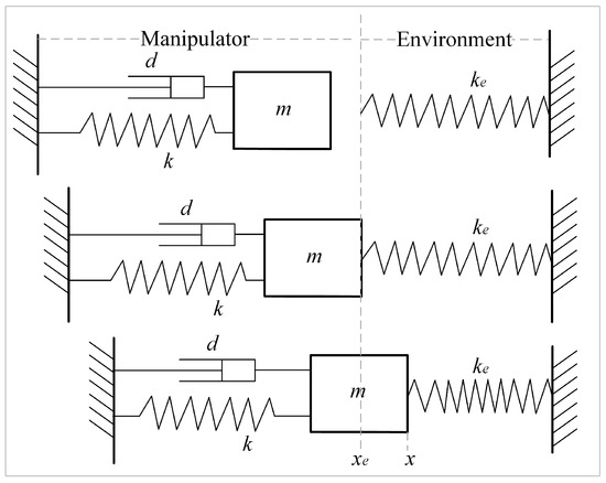
Figure 1.
System model of manipulator and rigid environment.
Figure 2 illustrates the contact force between the manipulator and the environment during the contact process. It can be observed that in the first stage, there was no contact between the manipulator and the environment. In the second stage, the manipulator underwent adjustments and stabilization, and in the third stage, the system reached a stable state. Since this paper focuses on the contact force between the manipulator and the environment, the primary focus is on the latter two stages.
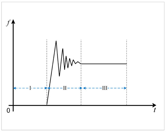
Figure 2.
The contact force between manipulator and environment.
2.2. Position-Based Impedance Control for Force Tracking
Because a robot is a rigid system that exhibits an overshoot when in contact with the environment, force feedback information is utilized to minimize the extent of the overshoot and demonstrate compliance during the contact phase. Similar to the earlier section, the contact model between the manipulator and the environment is depicted as a second-order mass–spring–damper system, as shown in Figure 3.
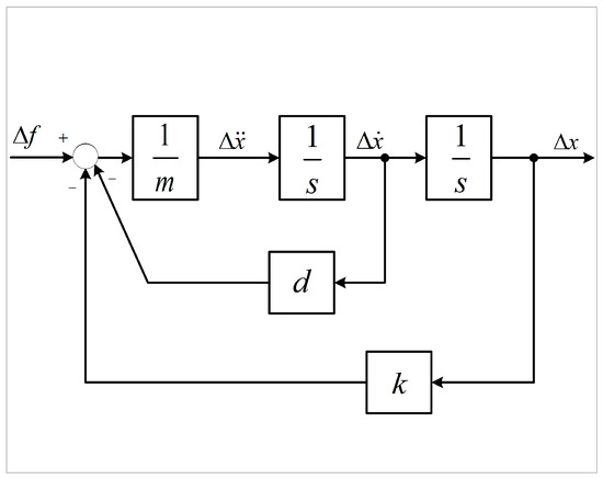
Figure 3.
Second-order system.
A significant body of literature demonstrates the widespread utilization of force-based impedance control for force tracking purposes. However, the majority of commercial robots solely offer position-based impedance control, rendering the achievement of force-based impedance control unfeasible with such robots. Nevertheless, position-based impedance control is commonly regarded as a means to enable compliant contact for robots. Position-based impedance control is illustrated in Figure 4.
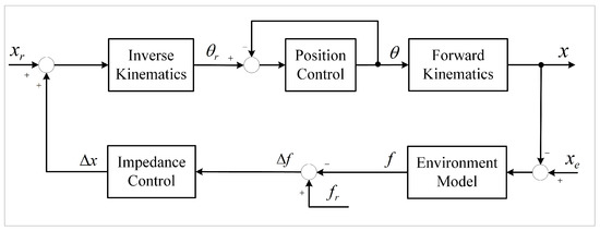
Figure 4.
The position-based impedance control schematic.
In Figure 4, and x denote the reference position trajectory and the actual output position trajectory of the manipulator, respectively. indicates the position of the environment. Since the environment is assumed to be rigid, it can be modeled as a spring with a stiffness of . The position compensation adheres to the impedance relation, expressed as follows:
where m, d, and k represent inertia, damping, and stiffness parameters, respectively. represents the discrepancy between the reference force and the actual feedback measurement value, given as , where is the designated reference force, f is the contact force of the end effector, and represents the error between the actual position and the reference position, expressed as .
The subsequent section involves the analysis of the steady-state error in impedance control. In general, the environmental model depicted in Figure 1 can be mathematically represented by Equation (2).
Based on Equation (2) and , the position of the end effector can be expressed as shown in Equation (3).
According to Equation (4), the steady-state error of the contact force can be expressed as Equation (5) when the manipulator is in a stable state.
However, considering the inherent difficulty of acquiring precise environmental stiffness and position information beforehand, the parameter deviation is employed to represent the actual parameters.
where represents the deviation in the environmental position, and represents the deviation in environmental stiffness. By replacing and with and , the steady-state error of the manipulator can be further expressed as shown in Equation (7).
3. Adaptive Controller
In this section, we discuss the model reference adaptive controller (MRAC) and the proposed variable universe fuzzy model reference adaptive impedance controller (VUF-MRAIC). We also demonstrate the stability conditions of the system when multiple variable parameters are present.
3.1. Model Reference Adaptive Controller
This study employs a single-input single-output (SISO) model reference adaptive controller, which refers to a control method that expects an ideal output for a controlled object with unknown parameters. By making the output of the reference model consistent with the output of the controlled object, the desired output is obtained. In this study, the basic structure of the model reference adaptive control system used when the coefficient of the controlled object is unknown is shown in Figure 5.
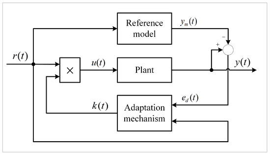
Figure 5.
Model reference adaptive control system.
In Figure 5, represents the control input, represents the actual output of the controlled object, represents the model output, represents the error equation, and denotes an adaptive adjustable coefficient. To ensure that the output of the reference model aligns with the actual output, adaptive control is achieved by adjusting the value of in the controller through an adaptive mechanism.
Now, considering a single-input single-output system, the controlled object and reference model can be represented by dynamic Equations (8) and (9).
where and are coefficient matrix Herwitz polynomials of the output system and input system, respectively. is the input of the reference model, and is the output of the reference model. In this context, p is the differential operator, and and are expressed by the following equations.
where , represents the coefficients of matrix elements, and n and q are the orders of higher-order derivatives. When the error is defined as , Equation (12) can be derived.
If it is determined that satisfies the condition where is strongly positive, based on , Equation (13) can be derived.
Subsequently, the control input and the coefficient adjustment rules are represented by Equations (14) and (15), respectively.
is a gain that can be defined as any value greater than zero. Furthermore, the derivative of the output is utilized to represent the state variable. The variables are represented as follows.
So, the linear combination of as a state variable can be obtained and expressed as in Equation (18).
Therefore, based on Equations (15) and (18), it can be concluded that the adaptive mechanism depicted in Figure 5 can be represented by Equation (19).
in Equation (19) is the obtained adaptive adjustable coefficient.
3.2. Variable Universe Fuzzy Controller
This section is divided into two parts: the introduction of the principles of the variable universe fuzzy controller and the design of the variable universe fuzzy controller.
3.2.1. The Principles of the Variable Universe Fuzzy Controller
According to the current research conducted by researchers, the real-time online adjustment of impedance parameters in impedance control is advantageous for accelerating the convergence of contact force and controlling it effectively. It is considered a highly effective control strategy. Therefore, building upon the model reference adaptive control discussed in the previous section, a variable universe fuzzy controller is introduced to dynamically adjust the impedance parameters d and k in real time, aiming to minimize errors.
A fuzzy controller is essentially an interpolator, and higher accuracy requires a greater number of control rules. However, implementing a large number of rules can pose challenges and hinder interpretability, as there is a limit to the number of rules that can be added indefinitely, leading to a phenomenon [27] known as “rule explosion”. The concept of variable universe fuzzy control was first introduced in reference [28], and its principle is illustrated in Figure 6. This approach involves altering the range of the universe to adjust the density of control rules. Contracting the universe is equivalent to adding more control rules, while expanding the universe is equivalent to reducing control rules. This technique enhances the sensitivity of the fuzzy controller.
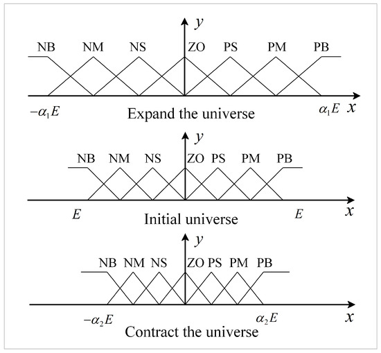
Figure 6.
Contraction and expansion of the universe.
3.2.2. Design of the Variable Universe Fuzzy Controller
However, the scaling factor of the universe plays a crucial role in determining the control accuracy. Therefore, the selection of the scaling factor is of great importance. Reference [28] imposes strict constraints on the choice of scaling factors. Currently, commonly used scaling factors include exponential and integral types.
Equations (20) and (21) represent the scaling factors for the variable universe fuzzy input, while Equation (22) represents the scaling factors for the variable universe fuzzy output. In previous research, researchers commonly utilized Equation (21) as the scaling factor for the variable universe fuzzy input. However, this expression includes two uncertain parameters, making it challenging to adjust these parameters during the actual application process. Moreover, performing integral or exponential operations at each step of the system may exceed the processing capacity of the processor. To simplify the process of obtaining the scaling factor, this paper adopts a two-stage fuzzy controller. The principle of the two-stage fuzzy controller is introduced below.
Considering the above explanation of the scaling factor, it is a very complicated process to understand the design of the scaling factor. The structure diagram of the two-stage fuzzy controller is shown in Figure 7.
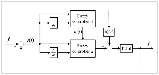
Figure 7.
Two-stage fuzzy controller.
The working principle of this two-stage fuzzy controller is as follows: Fuzzy controller 1 takes the input variables and , which represent the errors and the variation in the errors, respectively. Fuzzy controller 1 utilizes and to perform fuzzy inference and determine the scaling factor. The scaling factor is then applied to fuzzy controller 2 to achieve the contraction or expansion of the universe. In Figure 7, represents the output scaling factor of fuzzy controller 2, which is calculated in real time based on the system error. The design methods for fuzzy controller 1, fuzzy controller 2, and are discussed in the following sections.
For fuzzy controller 1, a dual-input single-output controller is considered. The error and the rate of change in error are utilized as inputs to fuzzy controller 1, and is employed as the output. The linguistic values of the input and output language variables are defined as three levels: “Big (B)”, “Medium (M)”, and “Small (S)”. The universe of the input variables and corresponds to the range of error and error change rate, which is defined as , and the universe of is . In this case, Gaussian functions are used as the membership functions for the input and output language variables of fuzzy controller 1, as depicted in Figure 8.
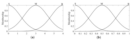
Figure 8.
(a) Membership function of input variable ; (b) the membership function of the output variable .
Given that the purpose of the universe scaling factor is to expand the universe of fuzzy controller 2 for large inputs and contract it for small inputs, the self-tuning rules can be formulated using the “IF THEN” format:
We take the larger of the inferred values and as the output of fuzzy controller 1, represented by Equation (23).
For fuzzy controller 2, a dual-input and single-output configuration is considered. The inputs are and , and the outputs are and . It is important to note that and are not output by the same fuzzy controller, but rather by two separate sets of fuzzy control systems. The initial universe of the input is , and the initial universe of the output is . So, the input universe of fuzzy controller 2 can be dynamically represented by , and the output universe of fuzzy controller 2 is . The selection of is slightly more complex, and should constantly change with the change in . When the error is large, the control effect is stronger, and when the error is small, the control effect is weaker. The fuzzy controller is a nonlinear function, so the selection of should also be nonlinear. After the simulation, selecting a proportional form of the scaling factor has a better effect, as shown in Equation (24).
where is the error E of the input to the fuzzy controller, is the universe corresponding to the input, is a positive number that is small enough, and is the universe scaling factor of the output obtained from the calculation. So, the input and output universes after scaling can be expressed as Equation (25).
and in the above equation represent the initial universes of the input and output, respectively. The input and output universes are described using seven levels: “Negative Big (NB)”, “Negative Medium (NM)”, “Negative Small (NS)”, “Zero (ZO)”, “Positive Small (PS)”, “Positive Medium (PM)”, and “Positive Big (PB)”. The membership function curves for the input and output language variables of fuzzy controller 2 are illustrated in Figure 9.
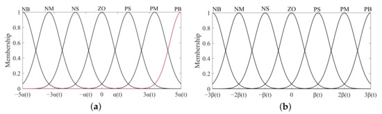
Figure 9.
(a) The membership function of the input and ; (b) the membership function of the output .
The rules of fuzzy controller 2 can be expressed in the form of as follows:
(1) the input is negative is negative, indicating that the force error is increasing, k increases and d decreases;
(2) the input is negative is positive, indicating that the force error is decreasing, k and d remain constant;
(3) the input is positive is positive, indicating that the force error is increasing, k decreases and d increases;
(4) the input is positive is negative, indicating that the force error is decreasing, k and d remain constant.
With the above design principle, the fuzzy rule set in Table 1 can be obtained by using the rules of fuzzy controller 2 and combined with control experience.

Table 1.
The fuzzy rule table for and .
The VUF-MRAIC control procedures proposed in this paper are summarized as follows:
Step 1: Use Equation (26) to obtain the values of the i-th input membership function of x and the j-th input membership function of y.
Step 2: Use to calculate the fuzzy output value, and calculate the k-th output membership function according to each rule as in Equation (27).
Step 4: Through the Defuzzification process of the barycenter method, obtain the outputs and , which are expressed in Equation (29), by using the reasoning result.
Step 5: Use Equation (30) to convert the output damping increment and stiffness increment into the actual contact force of the manipulator.
Figure 10 and Figure 11 are the flow chart of variable universe fuzzy control and the overall system diagram, respectively.
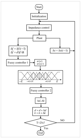
Figure 10.
Flow chart of variable universe fuzzy control.
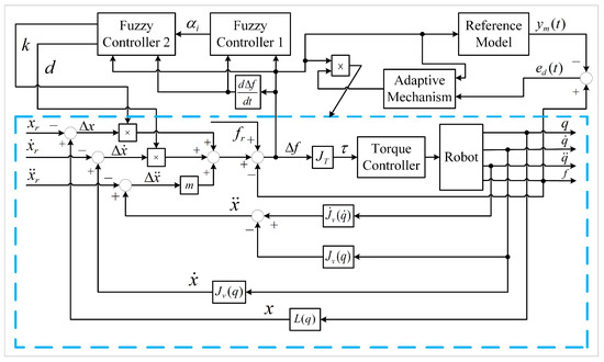
Figure 11.
Variable universe fuzzy model reference adaptive impedance control system block diagram.
3.3. Proof of System Stability Conditions
When researchers choose the inertia parameter M, damping parameter D, and stiffness parameter K to control the target system, if these parameters are constant and symmetric positive definite, the system exhibits asymptotic stability. However, in the proposed control method, the dynamic changes in the impedance parameters are taken into account through the variable universe fuzzy controller. In this case, M is constant, whereas both D and K become time-varying. Therefore, the stability of a system with multiple time-varying parameters needs to be considered.
Experience in variable stiffness impedance control has shown that reasonable variable stiffness does not exhibit a tendency toward instability. However, this study focuses on the simultaneous variation in damping and stiffness. Lyapunov functions are considered to determine system stability. In adaptive control, it is typical to construct an energy function that combines the weighted sum of the velocity error and position error. This approach can also be applied to varying stiffness and damping control. The Lyapunov function chosen for this purpose is displayed in Equation (31).
In the chosen Lyapunov function, represents the position error. It can be observed that by selecting certain positive constants , satisfies semi-positive definiteness for all . The selection of this function represents a generalized form of the Lyapunov function, enabling the establishment of adequate stability constraints, regardless of the system’s state. The following proof determines the conditions under which the system can achieve stability.
In Equation (31), represents a symmetric, semi-positive definite, and continuously differentiable matrix. Its differentiation can be performed by using Equation (32).
The impedance model can be represented by Equation (33).
By substituting from (33) into (32) and reorganizing it, Equation (34) can be obtained.
In order to eliminate the cross term between and , is defined as in the following Equation.
and are substituted into (34) to obtain Equation (37).
From the above calculation, it can be seen that when
is satisfied. According to the Lyapunov stability judgment theorem, the stability condition for the operation of this system is:
(1) is semi-negative definite.
(2) is semi-negative definite.
The controller parameters must satisfy the above conditions to ensure the stability of the variable damping and stiffness control system.
4. Dynamic Description of the Controlled System
The dynamics of a mechanical arm with n links are typically represented by the following equations:
where is an n-dimensional vector of generalized coordinates representing the joint angles of the links; is the positive definite mass matrix; represents the combined force of Coriolis and Centripetal forces, and here, is an matrix; is the vector containing the gravitational torques; is the friction vector; represents the external unknown disturbance vector, but in this case, we neglect external disturbances; and corresponds to the torque applied to each joint. By applying torque to each joint, the motion of the joints is driven, and by solving the aforementioned dynamic equations, the angle, velocity, and acceleration of each joint can be obtained.
The 6-DOF robot established in this paper follows the dynamic model based on the Lagrangian formulation.
is a matrix of , , and , with , , and corresponding to the angle, length, and mass of each joint, respectively. and are vectors about , , and . Table 2 shows the settings of the mechanical arm specifications.
Table 2.
Settings of mechanical arm specifications.
Figure 12 shows the mechanical model of the 6-dof robot arm described with Simulink. The input is the torque , that drives the motion of each joint, and the output is the of each joint angle and the position of the end effector. The inner loop controls the joint torque through a PID controller. The error between the output angle of the manipulator joint and the expected joint angle calculated by inverse kinematics is taken as the input of PID, and the torque control of the inner loop has been realized. For the processing of multiple sets of solutions, the angle range of each joint can be set at the beginning, and then solutions outside the joint range can be eliminated. First, the unique optimal solution of is determined, and then the optimal solution of is used to obtain the optimal solution of using the inverse solution method. The order of calculating the other joint angles is similar. The final set of solutions can serve as the control basis for achieving the robot’s target pose. The outer loop control is the VUF-MRAIC proposed earlier in this paper, which takes the actual output force f of the end effector as feedback information. So, the error between the actual force and the desired force is used as the input for the outer loop control, and the output is the position error of the end effector on the x-axis.
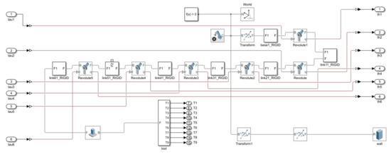
Figure 12.
Mechanical model in Simulink.
5. Simulation
Below, we describe three different simulation experiments that we conducted to test and compare the force tracking algorithms of the classical constant impedance control and the variable universe fuzzy model reference adaptive impedance control proposed in this paper in various environments. For reference, we have introduced the fuzzy terminal sliding-mode control in [15] as a reference. Classical constant impedance control adopts Equation (1), while adaptive variable impedance control adopts Equation (30). To compare and validate the algorithms, we utilized Matlab Simulink simulations. The simulations were conducted with the time step set to s.
5.1. Planar Environment
Assuming that the contact environment is a plane, . The environmental position is set to , the impedance coefficient is , and . The initial state : that is, the manipulator is not in contact with the environment in the initial state. The desired contact force is set to . The test results are shown in Figure 13. Figure 13a shows the trajectory tracking effect, and Figure 13b shows the force tracking effect.
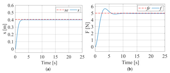
Figure 13.
Tracking effect when the contact environment is a plane. (a) Trajectory tracking effect; (b) force tracking effect.
After testing, selecting a damping coefficient of can achieve ideal results. In Figure 13, represents the location information of the environment; x represents the position information of the manipulator; represents the desired tracking force; and f represents the actual contact force between the manipulator and the environment. After contacting the environment, as shown in Figure 13a, it can be observed that there is no oscillation in the trajectory during the force adjustment process, and the desired trajectory corresponding to the desired force is tracked. The above results indicate that Equation (1) is robust to a plane with unknown environmental stiffness, making classical constant impedance control effective for force tracking in environments with unknown stiffness in the plane.
5.2. Inclined Plane Environment
Assuming that the contact environment is an inclined plane, and . This simulation compares the adaptability of three algorithms to dynamic changes in environmental positions, so the initial position is set to , the environmental stiffness is set to , and the impedance coefficients are set as above. Figure 14 is the trajectory tracking effect diagram corresponding to the three algorithms, and Figure 15 is the force tracking effect diagram corresponding to the three algorithms.
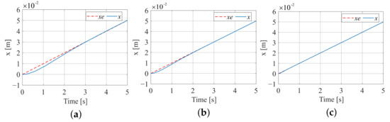
Figure 14.
Trajectory tracking effect when the contact environment is an inclined plane. (a) Constant impedance trajectory tracking; (b) fuzzy terminal sliding-mode trajectory tracking; (c) variable universe fuzzy model reference trajectory tracking.
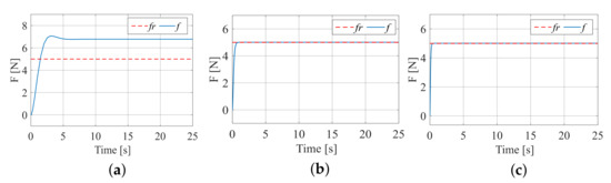
Figure 15.
Force tracking effect when the contact environment is an inclined plane. (a) Constant impedance force tracking; (b) fuzzy terminal sliding-mode force tracking; (c) variable universe fuzzy model reference force tracking.
For constant impedance control, after testing, selecting a damping coefficient can achieve stable force tracking. However, as shown in Figure 15a, the stable value is , and there is a significant deviation from the desired force tracking value. For adaptive variable impedance, after testing, selecting an initial damping coefficient of can achieve ideal results. As shown in Figure 15b,c, adaptive impedance control can achieve the desired stable value after a short period of time in the early stage. Therefore, for situations where the contact environment is inclined, adaptive variable impedance exhibits advantages over constant impedance control.
5.3. Sinusoidal Surface Environment
Assuming that the contact environment is a sinusoidal surface, and , and other settings and conditions are the same as above. Figure 16 shows the trajectory tracking effect of the three algorithms in this case, and Figure 17 shows the corresponding force tracking effect.

Figure 16.
Trajectory tracking effect when the contact environment is a sinusoidal surface. (a) Constant impedance trajectory tracking; (b) fuzzy terminal sliding-mode trajectory tracking; (c) variable universe fuzzy model reference trajectory tracking.
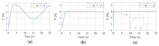
Figure 17.
Force tracking effect when the contact environment is a sinusoidal surface. (a) Constant impedance force tracking; (b) fuzzy terminal sliding-mode force tracking; (c) variable universe fuzzy model reference force tracking.
From Figure 17, it can be seen that for constant impedance, even with different values of d, the force tracking error persists, and the desired force cannot be achieved. However, for adaptive variable impedance, after testing, by selecting an initial damping coefficient of and a stiffness parameter of , the ideal tracking performance can be achieved. As shown in Figure 17b, the fuzzy terminal sliding-mode adaptive impedance control quickly tracks the desired force after a minor adjustment. In Figure 17c, the proposed variable universe fuzzy model reference adaptive impedance control achieves smooth contact. Overall, the latter two achieve the expected force tracking effect.
From the above three experiments, the following conclusions can be drawn: For a plane, even with uncertain environmental stiffness, constant impedance control can achieve the desired force tracking effect. However, for inclined planes or more complex unknown surfaces, constant impedance control is unlikely to achieve the desired force tracking effect. On the other hand, adaptive variable impedance control, after a short initial adjustment, can achieve the desired force tracking effect.
In this group of comparisons, by incorporating variable universe fuzzy control, the damping parameter d and stiffness parameter k were adjusted online. The dynamic curves of the damping and stiffness parameters after 25 s of simulation are shown in Figure 18.
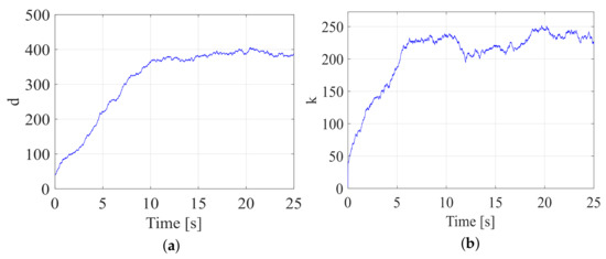
Figure 18.
The curves of adaptive parameters. (a) Adaptive damping parameters d; (b) adaptive stiffness parameters k.
It can be observed that the damping parameter and stiffness parameter are no longer fixed values but are dynamically updated online during the runtime. This dynamic variation in the impedance parameters enables the output force to move more rapidly toward the desired force direction.
6. Conclusions
Considering the shortcomings of traditional constant impedance control in the field of trajectory and force tracking, this study aimed to reduce the trajectory and force tracking errors of the system by developing a variable universe fuzzy model reference adaptive impedance controller. The innovation in this study is the determination of the most appropriate control parameters of the impedance controller by using a fuzzy controller in order to reduce the tracking error. For variable universe fuzzy controllers, a two-stage fuzzy controller is employed to obtain the universe scaling factor, which offers a simpler approach compared to other methods of selecting scaling factors. This method can achieve the effective trajectory tracking and force tracking of unknown environmental information in contact environments and enables the online automatic adjustment of impedance parameters. The stability of this controller is guaranteed by the Lyapunov function. Then, by comparing the simulation performance of the proposed variable universe fuzzy model reference adaptive impedance control strategy with constant impedance control and fuzzy terminal sliding-mode control in terms of trajectory and force, the superiority and effectiveness of the proposed strategy are demonstrated. The proposed controller was applied to a simulation model of a manipulator, and its performance on a plane, an inclined plane, and curved surfaces was tested. The results show that the variable universe fuzzy model reference adaptive impedance controller is more effective than the constant impedance controller. As a result of this study, it was concluded that the controller is valid.
Author Contributions
Conceptualization, Q.H.; methodology, Q.H.; software, D.K.; supervision, Q.H.; validation, D.K.; visualization, D.K.; writing—original draft, D.K.; writing—review and editing, D.K. and Q.H. All authors have read and agreed to the published version of the manuscript.
Funding
This research received no external funding.
Institutional Review Board Statement
Not applicable.
Informed Consent Statement
Not applicable.
Data Availability Statement
Not applicable.
Conflicts of Interest
The authors declare no conflict of interest.
References
- Abu-Dakka, F.J.; Saveriano, M. Variable impedance control and learning—A review. Front. Robot. AI 2020, 7, 590681. [Google Scholar] [CrossRef] [PubMed]
- Hogan, N. Impedance control: An approach to manipulation: Part III—Applications. J. Dyn. Syst. Meas. Control 1985, 107, 17–24. [Google Scholar] [CrossRef]
- Ding, Y.; Zhao, J.C.; Min, X. Impedance control and parameter optimization of surface polishing robot based on reinforcement learning. Proc. Inst. Mech. Eng. Part B J. Eng. Manuf. 2023, 237, 216–228. [Google Scholar] [CrossRef]
- Li, G.; Chen, X.; Yu, J.; Liu, J. Adaptive neural network-based finite-time impedance control of constrained robotic manipulators with disturbance observer. IEEE Trans. Circuits Syst. II Express Briefs 2021, 69, 1412–1416. [Google Scholar] [CrossRef]
- Peng, J.; Ding, S.; Yang, Z.; Xin, J. Adaptive neural impedance control for electrically driven robotic systems based on a neuro-adaptive observer. Nonlinear Dyn. 2020, 100, 1359–1378. [Google Scholar] [CrossRef]
- Kang, E.; Qiao, H.; Gao, J.; Yang, W. Neural network-based model predictive tracking control of an uncertain robotic manipulator with input constraints. ISA Trans. 2021, 109, 89–101. [Google Scholar] [CrossRef]
- Nazmara, G.; Fateh, M.M.; Ahmadi, S.M. Exponentially convergence for the regressor-free adaptive fuzzy impedance control of robots by gradient descent algorithm. Int. J. Syst. Sci. 2020, 51, 1883–1904. [Google Scholar] [CrossRef]
- Izadbakhsh, A.; Khorashadizadeh, S.; Ghandali, S. Robust adaptive impedance control of robot manipulators using Szász–Mirakyan operator as universal approximator. ISA Trans. 2020, 106, 1–11. [Google Scholar] [CrossRef]
- Bitz, T.; Zahedi, F.; Lee, H. Variable damping control of a robotic arm to improve trade-off between agility and stability and reduce user effort. In Proceedings of the 2020 IEEE International Conference on Robotics and Automation (ICRA), Paris, France, 31 May–31 August 2020; pp. 11259–11265. [Google Scholar]
- Zheng, K.; Zhang, Q.; Hu, Y.; Wu, B. Design of fuzzy system-fuzzy neural network-backstepping control for complex robot system. Inf. Sci. 2021, 546, 1230–1255. [Google Scholar] [CrossRef]
- Liu, A.; Chen, T.; Zhu, H.; Fu, M.; Xu, J. Fuzzy variable impedance-based adaptive neural network control in physical human–robot interaction. Proc. Inst. Mech. Eng. Part I J. Syst. Control Eng. 2023, 237, 220–230. [Google Scholar] [CrossRef]
- Huang, H.; Yang, C.; Chen, C.L.P. Optimal robot–environment interaction under broad fuzzy neural adaptive control. IEEE Trans. Cybern. 2020, 51, 3824–3835. [Google Scholar] [CrossRef]
- Ba, D.X. An intelligent sliding mode controller of robotic manipulators with output constraints and high-level adaptation. Int. J. Robust Nonlinear Control 2022, 32, 6888–6912. [Google Scholar] [CrossRef]
- Liu, H.; Sun, J.; Nie, J.; Zou, L. Observer-based adaptive second-order non-singular fast terminal sliding mode controller for robotic manipulators. Asian J. Control 2021, 23, 1845–1854. [Google Scholar] [CrossRef]
- Ozguney, O.C.; Burkan, R. Fuzzy-terminal sliding mode control of a flexible link manipulator. Acta Polytech. Hung. 2021, 18, 179–195. [Google Scholar] [CrossRef]
- Rojas-García, L.; Bonilla-Gutiérrez, I.; Mendoza-Gutiérrez, M.; Chávez-Olivares, C. Adaptive force/position control of robot manipulators with bounded inputs. J. Mech. Sci. Technol. 2022, 36, 1497–1509. [Google Scholar] [CrossRef]
- Chen, J.; Tao, G. Adaptive Control of Robot Manipulators in Varying Environments. In Proceedings of the 2022 Systems and Information Engineering Design Symposium (SIEDS), Charlottesville, VA, USA, 28–29 April 2022; pp. 211–216. [Google Scholar]
- Cao, F.; Docherty, P.D.; Ni, S.; Chen, X. Contact force and torque sensing for serial manipulator based on an adaptive Kalman filter with variable time period. Robot. Comput.-Integr. Manuf. 2021, 72, 102210. [Google Scholar] [CrossRef]
- Mazare, M.; Tolu, S.; Taghizadeh, M. Adaptive variable impedance control for a modular soft robot manipulator in configuration space. Meccanica 2022, 57, 1–15. [Google Scholar] [CrossRef]
- Xu, K.; Wang, S.; Yue, B.; Wang, J.; Peng, H.; Liu, D.; Chen, Z.; Shi, M. Adaptive impedance control with variable target stiffness for wheel-legged robot on complex unknown terrain. Mechatronics 2020, 69, 102388. [Google Scholar] [CrossRef]
- Wei, J.; Yi, D.; Bo, X.; Guangyu, C.; Dean, Z. Adaptive variable parameter impedance control for apple harvesting robot compliant picking. Complexity 2020, 2020, 4812657. [Google Scholar] [CrossRef]
- Ajani, O.S.; Assal, S.F.M. Development of an autonomous robotic system for beard shaving assistance of disabled people based on an adaptive force tracking impedance control. Proc. Inst. Mech. Eng. Part C J. Mech. Eng. Sci. 2021, 235, 5758–5775. [Google Scholar] [CrossRef]
- Jiao, C.; Yu, L.; Su, X.; Wen, Y.; Dai, X. Adaptive hybrid impedance control for dual-arm cooperative manipulation with object uncertainties. Automatica 2022, 140, 110232. [Google Scholar] [CrossRef]
- Fereydooni, R.H.; Siahkali, H.; Shayanfar, H.A.; Mazinan, A.H. sEMG-based variable impedance control of lower-limb rehabilitation robot using wavelet neural network and model reference adaptive control. Ind. Robot Int. J. Robot. Res. Appl. 2020, 47, 349–358. [Google Scholar] [CrossRef]
- Zhang, J.; Li, H.; Liu, Q.; Li, S. The model reference adaptive impedance control for underwater manipulator compliant operation. Trans. Inst. Meas. Control 2023, 45, 2135–2148. [Google Scholar] [CrossRef]
- Omrani, J.; Moghaddam, M.M. Nonlinear time delay estimation based model reference adaptive impedance control for an upper-limb human-robot interaction. Proc. Inst. Mech. Eng. Part H J. Eng. Med. 2022, 236, 385–398. [Google Scholar] [CrossRef]
- Weinschenk, J.J.; Weinschenk, J.; Combs, W.E.; Marks, R.J. Avoidance of rule explosion by mapping fuzzy systems to a union rule configuration. In Proceedings of the 12th IEEE International Conference on Fuzzy Systems, 2003, FUZZ ‘03, St. Louis, MO, USA, 25–28 May 2003; Volume 1, pp. 43–48. [Google Scholar]
- Li, H. Adaptive fuzzy controllers based on variable universe. Sci. China Ser. E Technol. Sci. 1999, 42, 10–20. [Google Scholar] [CrossRef]


Disclaimer/Publisher’s Note: The statements, opinions and data contained in all publications are solely those of the individual author(s) and contributor(s) and not of MDPI and/or the editor(s). MDPI and/or the editor(s) disclaim responsibility for any injury to people or property resulting from any ideas, methods, instructions or products referred to in the content. |
© 2023 by the authors. Licensee MDPI, Basel, Switzerland. This article is an open access article distributed under the terms and conditions of the Creative Commons Attribution (CC BY) license (https://creativecommons.org/licenses/by/4.0/).