Abstract
To address the demand for low noise and high stealthiness in ships and other vessels, this paper innovatively proposes an inertial magnetic levitation actuator based on non-uniform-sized Halbach permanent magnet arrays. To improve control accuracy, it is necessary to establish an accurate analytical model of the magnetic field and then obtain an accurate electromagnetic force model. However, the distortion of the magnetic field at the ends produces end effects, resulting in thrust fluctuations that affect the actuator’s control accuracy. Therefore, considering the end effects is necessary to establish an accurate analytical model of the magnetic field. To analyze the end leakage magnetic field of the Halbach array, the concept of a mechanical pseudo-cycle in the actuator is proposed, and the cycle of a Fourier series is redefined. A completed analytical expression of the Halbach array magnetic field distribution is derived by the new Fourier series, in which the end leakage magnetic field is contained. The accuracy of the proposed method is verified by solving the analytical model of the magnetic field, and the analytical results are compared with finite element simulations and experimental tests.
1. Introduction
The advancement of ships is closely related to their acoustic performance [1,2,3]. The impact of ship noise can be categorized into three main aspects: (1) It affects comfort and the reliability of electronic equipment. (2) It causes acoustic pollution in the marine environment, harming the surrounding marine ecosystem. (3) It reduces the stealth performance of military vessels, significantly affecting combat effectiveness and survival capabilities. Therefore, research into ship vibration and noise reduction technologies holds substantial commercial and military value.
The propulsion shaft system is the core of the ship’s power system, and the vibration and noise it generates are major contributors to the ship’s underwater acoustic radiation. Magnetic levitation actuators, with their wide control bandwidth and fast response speed, can be used for vibration control of high-stiffness, large-mass equipment such as shaft systems [4]. However, existing magnetic levitation actuators do not yet meet the requirements for controlling the lateral vibrations of shaft systems in terms of output force, thermal performance, and control stability. Enhancing the thrust density of magnetic levitation actuators, improving their dynamic characteristics, optimizing heat dissipation, and refining magnetic field distribution are current research focuses. The performance optimization of magnetic levitation actuators largely depends on their magnetic field distribution, making the establishment of an accurate analytical model of the magnetic field highly significant.
The Halbach array, an innovative type of permanent magnet array proposed by American scholar Klaus Halbach [5], features an internal magnetization direction that changes continuously at an angle. By arranging the permanent magnets appropriately, the magnetic field in the air gap can be enhanced, thereby increasing the thrust density of magnetic levitation actuators.
Halbach arrays in actuators increase field concentration and reduce leakage. However, practical Halbach arrays usually use segmented permanent magnets instead. The assembly of segmented permanent magnets affects the continuity and stability of the magnetic field. Therefore, the modeling and simulation of segmented permanent magnets need to comprehensively consider factors such as material properties, magnetic field distribution, and manufacturing processes.
The analytical modeling of the magnetic field in Halbach arrays typically employs methods such as the equivalent magnetic charge method [6,7], the equivalent current method [8,9,10], and the sinusoidal approximation method [11,12,13,14]. Ham, C et al. used the magnetic charge method to establish an analytical model for a single magnet and derived the magnetic field of the permanent magnet array through superposition [15]. This method can describe the magnetic field distribution at the ends of the permanent magnet array, but it involves significant computational complexity. Furlani, E P. [16], based on Ampere’s molecular current hypothesis, replaced the permanent magnet field with a surface current field and used the method of mirror image to substitute the magnetic yoke, calculating the magnetic field of the Halbach array without considering end effects and leakage flux. Jiang, Y et al. developed a magnetic field distribution model for a dual-layer permanent magnet structure using the sinusoidal model [17]. While the sinusoidal method is intuitive, it assumes that the Halbach array’s magnetic field consists of infinite sinusoidal harmonics, neglecting the presence of end harmonics, resulting in significant errors for shorter magnet lengths. Thus, the sinusoidal method is suitable only for arrays with long lengths and many pole pairs [18]. Yu-Jing Song et al. derived a mathematical analytical model for periodic Halbach arrays using Fourier series and spatial integration techniques [19]. Compared to finite element simulations, this model achieves fast solution speed. However, the Halbach array represents an ideal permanent magnet arrangement. Due to individual magnet differences and assembly errors, the actual magnetic field strength is weaker than the ideal case. All these characteristics are not typically captured by an analytical model based on some simplifying assumptions. While finite element simulations can provide a magnetic field model [20,21,22], their accuracy is influenced by mesh quality, and they require significant computational time.
It is noteworthy that in magnetic levitation actuators, the limited mechanical dimensions of the mover’s permanent magnet array lead to significant nonlinear distortion in the magnetic field distribution at the ends of the magnets. This affects the performance and stability of the actuator and poses considerable challenges for its control [23]. Therefore, it is crucial to study the end effect modeling methods to accurately describe the magnetic field distribution characteristics in the end regions. However, there are few reports on this topic in the existing literature. This paper innovatively proposes an inertial magnetic levitation actuator structure based on a non-uniform Halbach array and establishes an analytical model of the magnetic field that considers end effects. This model provides a theoretical foundation for thrust modeling, structural optimization, and controller design. Thus, this paper uses the concept of a pseudo-period to study finite-length Halbach permanent magnet arrays. A modified Fourier series is used to establish an analytical mathematical model of the magnetic field within the pseudo-period, considering end effects. The accuracy of the proposed magnetic field modeling method is verified through comparisons with magnetic field simulation calculations and experimental tests.
2. Magnetic Field Modeling
2.1. Magnetic Levitation Actuator Based on Halbach Array
Under the same amount of permanent magnetic material, a magnetic levitation actuator with a Halbach permanent magnet array achieves higher magnetic flux density and lower iron loss, with a magnetic field distribution closer to a sinusoidal form. In a moving-magnet structure, the yoke and permanent magnets act as the mover, while the coils and coil support function as the stator. Due to the larger mass of the mover, its mechanical strength is ensured when used in shaft vibration reduction systems. However, it is crucial to prevent the permanent magnets from damage or demagnetization due to severe vibrations.
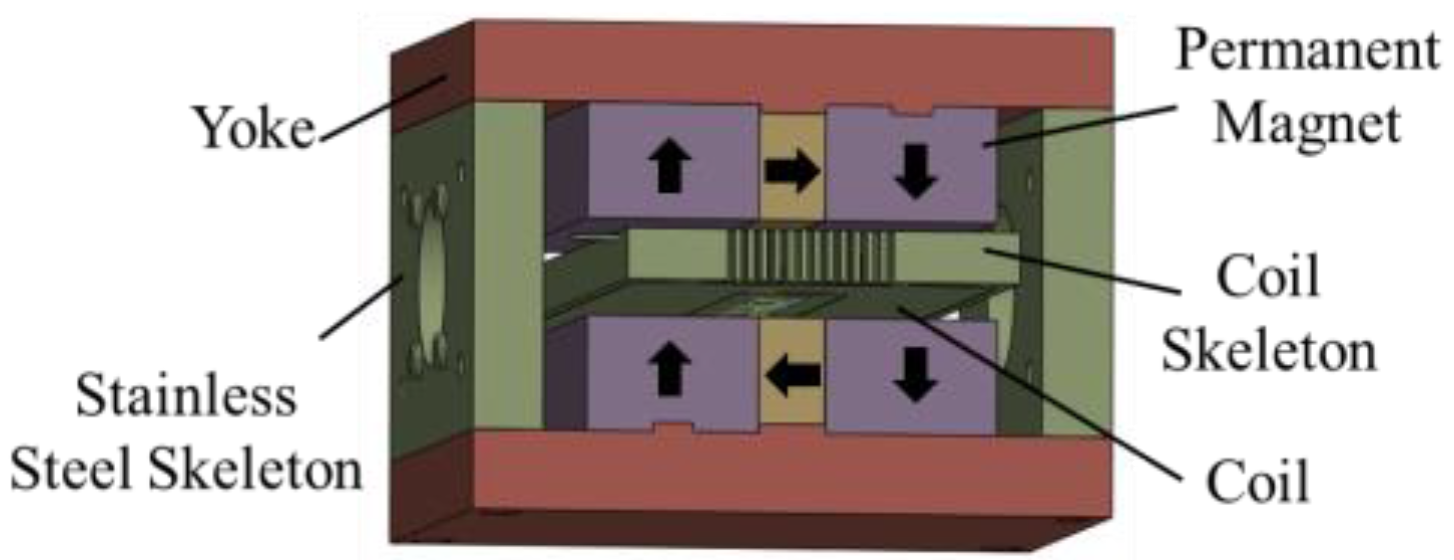
The basic structure of the magnetic levitation actuator is shown in Figure 1. This actuator consists of a coil stator and a Halbach permanent magnet array mover. The coils are cross-wound with enameled wire, offering a high slot fill factor, high precision in coil processing and assembly, and ease of installation. The coils in the actuator’s working area are regular straight conductors, which avoids the issue of difficult modeling associated with irregular coils. The coil frame is equipped with cooling fins to ensure the magnetic levitation actuator operates normally. The magnetization direction within the Halbach array permanent magnets changes continuously by 90° along the yoke. Neodymium iron boron (NdFeB) was selected as the permanent magnetic material for the actuator due to its high coercivity, remanence, and magnetic energy product, effectively enhancing the thrust-to-volume ratio of the linear actuator. The yoke is made of pure iron to guide the magnetic field and form a closed magnetic circuit. The Halbach permanent magnet array produces a stable magnetic field. The powered coil is placed in the magnetic field in which the force is calculated as F = nBIL, where F can be regarded as the force of the actuator; n is the number of turns of the coil, B is the magnetic field in which the wire is located and L is the length of the wire in the magnetic field.
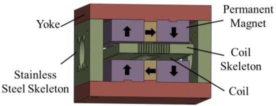
Figure 1.
Three-dimensional view of the magnetic levitation actuator.
We have studied the influence of the width ratio between horizontally and vertically magnetized permanent magnets on the air-gap magnetic field. It was found that when the width ratio is approximately 3, the linearity of the air-gap magnetic field reaches its peak, and the magnetic field strength is relatively high. A parametric design model of the non-uniform Halbach actuator is established, with parameters optimized using a genetic algorithm. The principle of magnetic field modulation is employed to achieve low-speed high-thrust control and direct-drive structural design, further improving the transmission efficiency of the actuator system and reducing system complexity. Multi-layer coils are assembled on the stator, and by altering the coil current, Lorentz forces drive the mover of the Halbach permanent magnet array magnetic levitation actuator, enabling single-degree-of-freedom linear motion of the mover.
2.2. Analytical Modeling in the Magnetic Field in Non-Uniform Halbach Arrays
2.2.1. Fourier Magnetic Field Analysis of a Complete Pole Pitch Halbach Array Using Pseudo-Period and Image Methods
Due to the presence of end effects, the magnetic field in a Halbach permanent magnet array does not exhibit strict periodicity but may display certain quasi-periodic characteristics. The pseudo-period method aims to approximate these non-periodic magnetic field distributions [24].
To establish an analytical magnetic field model that considers end effects, we define the pseudo-period, as shown in Figure 2, where represents the total distance over which the magnetic field at the end decays to zero. In defining the pseudo-period, we treat the permanent magnet array in the magnetic levitation actuator as a whole, forming a new array composed of an infinite number of original permanent magnet arrays.
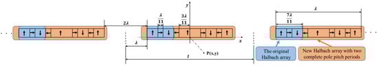
Figure 2.
Schematic structure of one-dimensional Halbach permanent magnet array based on pseudo-cycle.
If the pole pitch of the permanent magnet array is , the symmetry period of the air-gap magnetic density in the sine-like zone is still . Still, the air-gap magnetic density in the end distortion zone does not follow this symmetry law. Define as the distance from the edge of the permanent magnet array when the magnetic field decays to zero. Based on the results of the finite element static magnetic field simulation, it can be approximated as , i.e., the magnetic fields do not affect each other when the distance between two adjacent permanent magnet arrays is . Thus, the period of the new array, or the pseudo-period for the permanent magnet array in the magnetic levitation actuator, is . In this study, the permanent magnet array consists of non-uniform Halbach magnets, with the transverse magnetized permanent magnet length and the vertical magnetized permanent magnet length .
Since the Halbach is periodic, the Fourier series is used to represent the magnetization. Figure 2 depicts the structure of the Halbach permanent magnet array, which repeats two wavelengths, each containing four magnets. The direction of the arrow in the diagram represents the direction of magnetisation of the permanent magnet. A new pseudo-period consists of nine magnets, including one shared central magnet (precisely spanning two wavelengths) to create a symmetric configuration, with the magnets at both ends magnetized vertically.
Given that the system approximates a quasi-static magnetic field, Maxwell’s equations can be expressed as:
where is the free current density.
In the region of permanent magnets, there are no free currents, thus . For a magnetized material with a magnetization , the relationship between the magnetic flux density and the magnetization is given by:
Since the divergence of a curl is always zero, we can define the magnetic vector potential such that:
Thus,
In a static magnetic field, applying the Coulomb gauge , we have:
Using Equations (1)–(4), we derive the Poisson’s equation:
In the Cartesian coordinate system (xyz), scalar Poisson’s equation for the y-component of the magnetic vector potential is:
where Mn is the nth Fourier component of M.
The magnetization components along the horizontal direction x and the vertical direction z can be represented using Fourier coefficients and :
where the spatial wave number of the nth harmonic is , the magnetization intensity along the x and z directions in Fourier series form is:
As long as the vector magnetic momentum A is solved, the expression for the magnetic induction strength B can be obtained by using Equation (4), which in turn leads to the force model of the permanent magnet array actuator.
The magnetic vector potential is
According to the literature [25], the magnetic field distribution on the lower surface of the permanent magnet array can be derived as
where , and the height of the permanent magnet is .
Then, the Fourier series of the magnetic field distribution at z below the permanent magnet array (on the strong magnetic field side) is
The magnetic flux density is expressed as
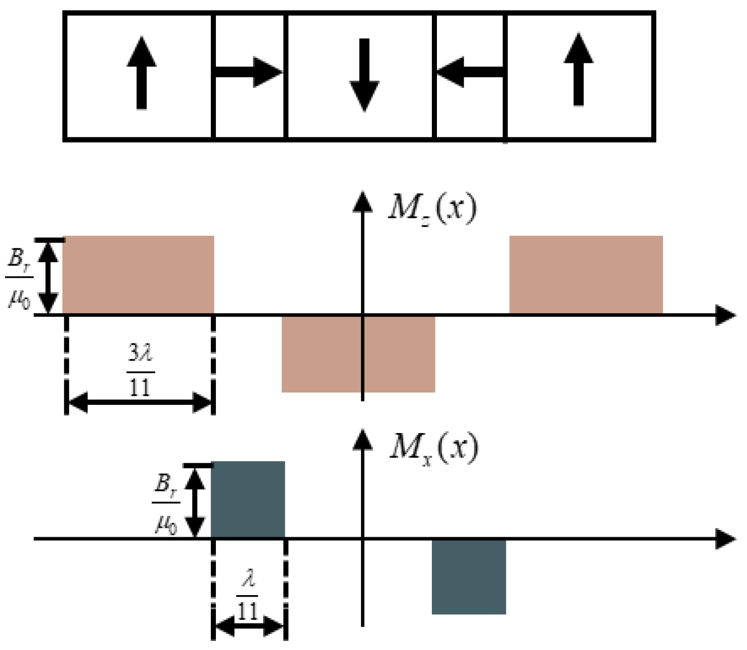
The magnetization vector is often used to describe the magnetization state of the magnetic medium, and its value is related to the spatial distribution of the permanent magnets in Halbach permanent magnet arrays. The spatial distribution of the magnetization vector is shown in Figure 3 for Halbach arrays neglecting the end effect.
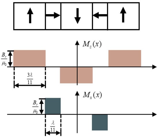
Figure 3.
Spatial distribution of magnetic field strength.
For a one-dimensional Halbach permanent magnet array of infinite length, the magnetization strength M can be expressed as:
where k is an arbitrary integer, and is the remanence of the permanent magnet.
Substituting Equation (14) into Equation (10) so that l = λ, the expression for the coefficients of the Fourier series of the magnetization under the pseudo-period is deduced as:
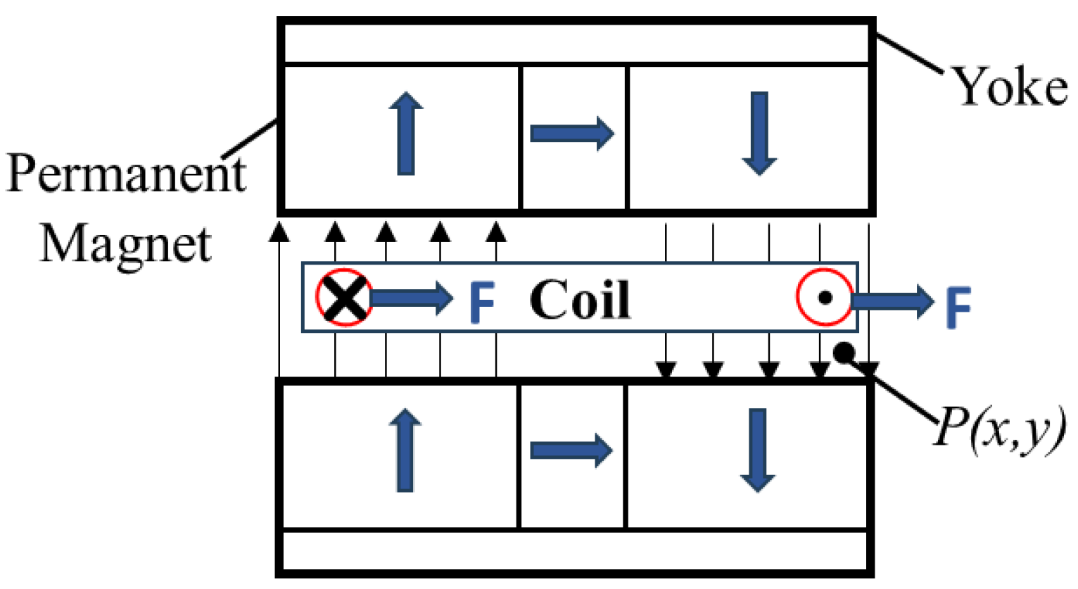
The analytical model for the magnetic flux density at point P below the upper part of the permanent magnet array in Figure 2 is provided below. Figure 4 illustrates a schematic diagram of the magnetic levitation actuator model. The analytical model for the magnetic flux density at point P above the lower part of the permanent magnet array can be similarly derived. Thus, the total magnetic flux density distribution of the Halbach permanent magnet array is .
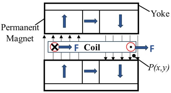
Figure 4.
Schematic diagram of the magnetic levitation actuator model.
Substituting Equation (15) into Equation (12), an analytical expression of the magnetic induction B at the point P (x, y) for a one-dimensional Halbach array of width λ shown in Figure 3 is derived:
where .
For a one-dimensional Halbach PM array of finite width, let l = 4λ, and derive the analytical expression of the magnetic flux density for a one-dimensional Halbach PM array of width 2λ shown in Figure 2:
where
The surface current method, based on Ampere’s circuital law, treats the magnetization vector of the permanent magnet as an equivalent current distribution, simplifying the magnetic flux density calculation. This method is intuitive and has clear physical significance [16]. However, for periodic magnetic flux density distributions such as those in Halbach arrays, the Fourier analysis method is more effective and simpler. Through decomposition and superposition, it can very accurately describe complex magnetic flux density distributions.
2.2.2. Analytical Model of Halbach Array Magnetic Flux Density Based on the Surface Current Method
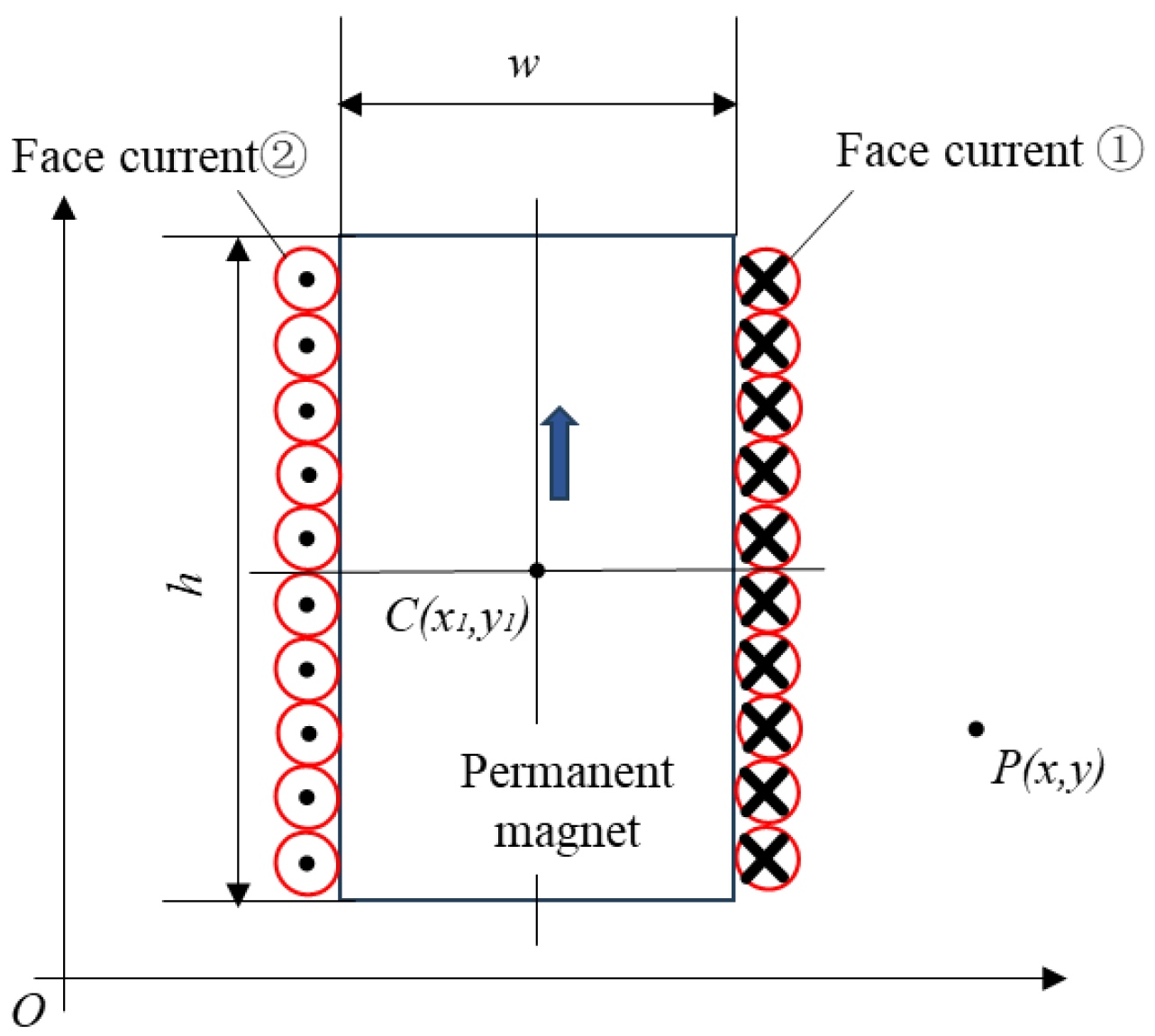
The magnetic field of the Halbach array permanent magnets was calculated based on the amperometric molecular current hypothesis, using the surface current field instead of the permanent magnet field and the universal mirror method instead of the yoke. The surface current along the y-axis is shown in Figure 5, and the direction of magnetisation is shown in Figure 5.
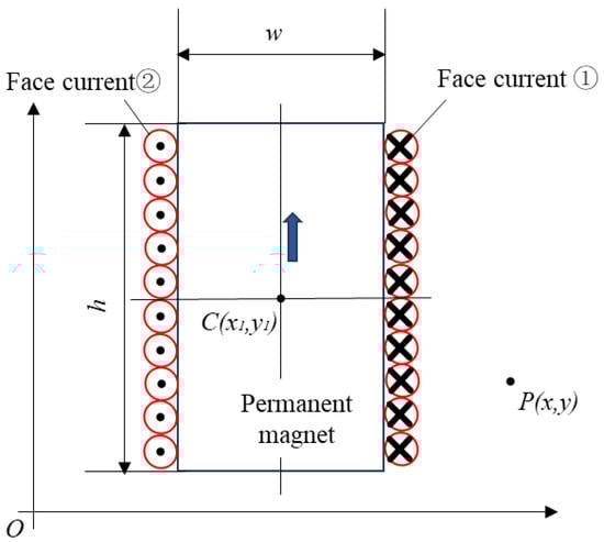
Figure 5.
Schematic diagram of the equivalent surface current for y-direction magnetization.
From reference [26], the magnetic flux density generated by the surface current ➀ at a point in space is obtained as
where (x1, y1) denotes the coordinates of the center position of the permanent magnet, (x, y) denotes the coordinates of the position of any point in the space, h is the thickness of the permanent magnet, w is the width of the permanent magnet, and the surface current density is assumed to be KI.
Similarly, the magnetic flux density generated by surface current 2 should be
Thus, it can be derived that the magnetic flux density produced by a single permanent magnet magnetized along the y-direction at a point P (x, y) in the space is
where, in , the first subscript y denotes the magnetization along the y direction and the second subscript x denotes the component along the x direction.
According to Equation (20), the equivalent surface current distribution for the magnetic flux density of a single permanent magnet depends solely on the spatial coordinates, dimensions (width and thickness), and the magnetization intensity of the permanent magnet.
When the permanent magnet is placed between ferromagnetic yokes, the magnetic flux density distribution is no longer that of free space. Assuming infinite relative permeability of the yokes, the magnetic vector potential at the contact surface between the yokes and the permanent magnet will differ from that within the permanent magnet. This creates equivalent currents at the contact surfaces, complicating the analysis and calculations. To address this, the mirror image method is commonly used to account for the influence of the magnetic yokes. In this method, the yokes are replaced by multiple image sources, simplifying the magnetic field distribution to that of the permanent magnet in free space. The principle of the mirror image method is illustrated in Figure 6. Figure 6 illustrates a permanent magnet QI positioned between two parallel magnetic yokes, separated by a distance d.
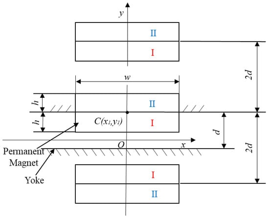
Figure 6.
Schematic diagram of the mirror image method.
The first image source QII, sharing the same y-direction magnetization, is created by the magnetic yoke in contact with QI. Next, QI and QII are mirrored by the second magnetic yoke, creating the subsequent image source below. This iterative process generates an infinite series of image sources, each spaced by 2d. The magnetic flux density distribution at any point in space is the superposition of the fields from these permanent magnets and their image sources at that point. If the central coordinates of the first group (QI and its image source QII) are C (x1, y1), the magnetic flux density distribution at point P (x, y) in space can be determined using Equations (18)–(20).
If the magnetization direction is the x direction, the coordinates of the center position of the whole image composed of the first group of permanent magnets QI and the mirror source QII are C (x1, y1), and similarly, it can be derived that the magnetic flux density of the permanent magnets and their mirror source at a point P (x, y) in the space is
The total magnetic flux density distribution at a specific point in space can be calculated using Equations (21) and (22), which involve summing the magnetic flux density of each permanent magnet and their image sources. Previously, based on the Amperian current hypothesis, the equivalent surface current method was used to replace the permanent magnets, deriving the magnetic flux density distribution expression for a single permanent magnet in space. Subsequently, the image method was used to replace the magnetic yokes, simplifying the calculation and obtaining the spatial magnetic flux density distribution expression for the sources composed of permanent magnets and their image sources.
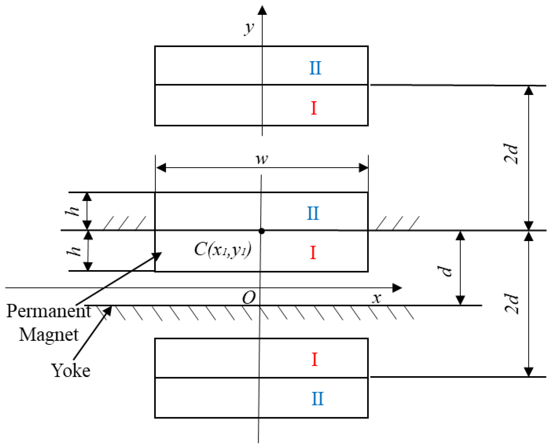
Each row in Figure 7 forms a Halbach array; therefore, the whole structure is made up of a pair of Halbach arrays. To investigate the impact of geometric parameters of the air-gap magnetic field on field strength and linearity, a Cartesian coordinate system was established with the center of the air-gap magnetic field in the z-axis direction as the origin. The geometric dimensions of each permanent magnet were set as variable parameters, creating a parametric model of the non-uniform-size Halbach array magnetic field, as shown in Figure 7. In Figure 7, a represents the width of the horizontally magnetized permanent magnets, b represents the width of the vertically magnetized permanent magnets, and 2d is the distance between the two parallel magnetic yokes. The dimensional parameters of the permanent magnets used in the calculations for the non-uniform-size Halbach array are numbered according to their different magnetization directions. The geometrically parameterized boundary coordinates of the permanent magnets on the coordinate axes are expressed as follows.
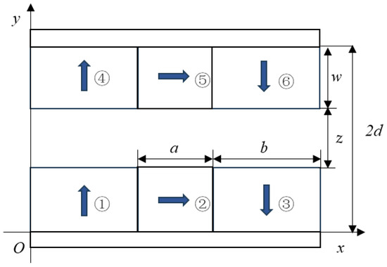
Figure 7.
Parametric model of the non-uniform-size Halbach array.
The air-gap magnetic flux density of a non-uniform-size Halbach array adheres to the principle of superposition of magnetic flux density. Based on the derivation of the analytical expression for a single rectangular permanent magnet, the parametric analytical expression for the air-gap magnetic flux density of a non-uniform-size Halbach array can be obtained:
The pseudo-period concept has been introduced before to account for the end effects of Halbach arrays; now it is noted that this cannot be described when using the surface current method. The end effect typically results in attenuation or distortion of the magnetic field at the edges or ends of the magnets, which often extends beyond the descriptive accuracy of the surface current method.
2.3. Finite Element Simulation
To validate the accuracy of the proposed analytical model, finite element software is used to calculate the magnetic flux density distribution of the Halbach permanent magnet array, and the results are compared with the model calculations. The parameters of the permanent magnet array are listed in Table 1, with λ = 154 mm, Br = 1.23 T, d = w +z = 48 mm. The permanent magnet material used for the array is NdFe38. A finite element simulation model is established in Maxwell-2D, as shown in Figure 8. The magnetic levitation actuator exhibits significant magnetic flux density distortion at the ends, making it essential to consider the end effect in high-precision control scenarios.

Table 1.
Basic dimensions and related data of Halbach array maglev actuator.
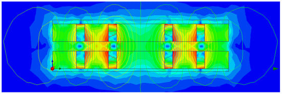
Figure 8.
Finite element simulation model.
Results obtained from the analytical model (Fourier analysis + surface currents) are compared to numerical results from FEA, as shown in the figure below.
Initially, an attempt was made to consider three permanent magnets as one period of the model, but significant errors were observed, as illustrated in Figure 9.
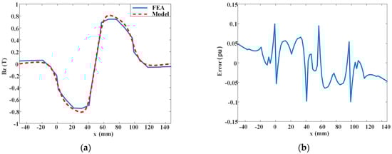
Figure 9.
Modeling of magnetic flux density based on Fourier analysis (original three arrays for one cycle). (a): Comparison of non-uniform-sized Halbach permanent magnet arrays, (b): error diagram.
Based on the findings from reference [19], a period usually refers to the pole pitch of a permanent magnet array, i.e., the distance between two magnets with the same magnetization direction. However, the model discussed in this paper only includes three permanent magnets, which cannot form a complete pole pitch period. Therefore, five additional permanent magnets were added to the right end of the original permanent magnet array to form two complete pole pitch periods for establishing the magnetic field model.
The magnetic field models of the one-dimensional Halbach permanent magnet array, considering and ignoring the end effects, were analyzed and solved, respectively. The comparison results are shown in Figure 10. The comparative analysis revealed that the relative error with the simulation results is significantly smaller when considering two pole pitches as one period compared to considering three permanent magnets as one period.

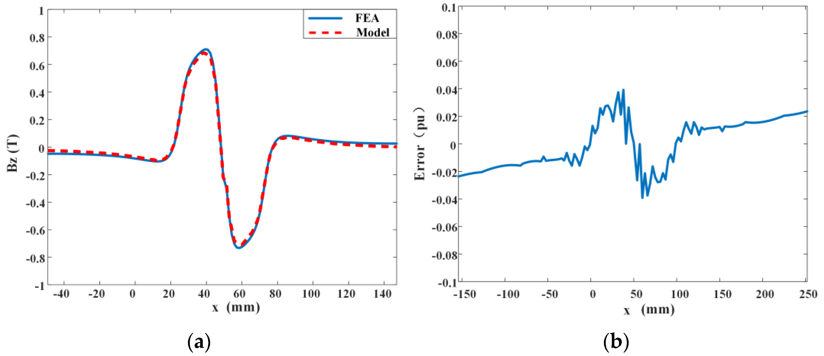
Figure 10.
Modeling of magnetic flux density based on Fourier analysis (make up five permanent magnets to make up two pole spacings, one cycle for one pole spacing). (a): Comparison of finite element and analytical solutions for air-gap magnetic flux density of permanent magnets, (b): error diagram.
Furthermore, the study focused on the magnetic field model comprising two pole pitches within one period, deriving the magnetic flux density distribution formulas while considering and ignoring the end effects. As depicted in Figure 10, the analytical method considering the end effects closely aligns with the finite element simulation curves, verifying the accuracy of the proposed model.
However, the addition of permanent magnets on the right side significantly affects the magnetic flux density distribution of the original array’s right half. To enhance the accuracy of the results, a method was employed where the magnetic flux density distribution of the original left half is mirrored onto the right side and taken as negative. The overall magnetic flux density distribution obtained using this method is illustrated in Figure 11.

Figure 11.
Magnetic field modeling by combined mirror method and Fourier analysis. (a): Comparison of non-uniform-sized Halbach permanent magnet arrays, (b): error diagram.
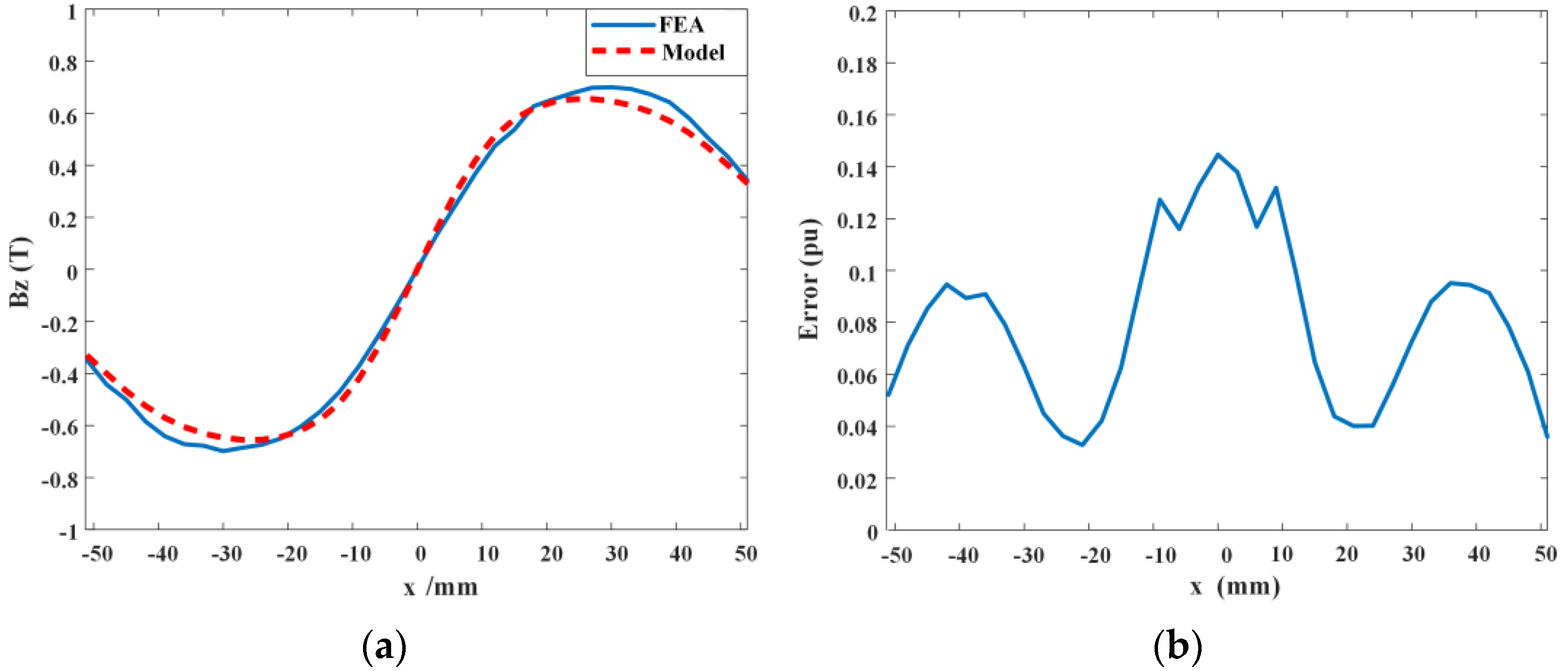
Using both the surface current method and the Fourier analysis method to establish magnetic field analytical models for the Halbach array, it is evident from Figure 12 that the surface current method does not fully account for end effects. As seen from the comparison in Figure 10, within the interval −λ < x < λ, the finite element simulation results without considering end effects closely match the analytical model results, exhibiting well-defined quasi-sinusoidal distribution characteristics. However, beyond this region, the magnetic field analytical results for an infinitely long and wide Halbach permanent magnet array, without considering end effects, do not have practical significance compared to the finite element simulation results. The red line in Figure 10 illustrates the magnetic field analytical results considering end effects alongside the finite element simulation results. The following conclusions can be drawn from the figure. For Bz, the maximum absolute error is 0.03925 T, the average absolute error is 0.0161 T, and the average relative error is 5.1517%. This error is mainly due to the truncation error in the magnetic field analytical model, which only considers contributions up to the highest order of 200. In practical applications, this error range is acceptable, confirming the accuracy of the magnetic field analytical model.
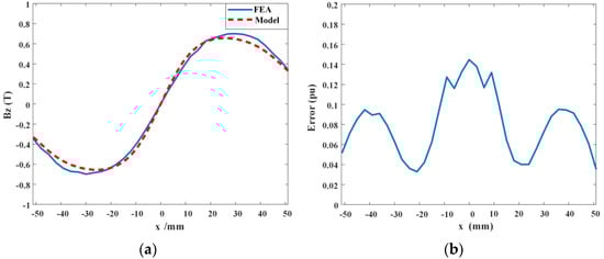
Figure 12.
Magnetic field modeling based on the surface current method. (a): Comparison of non-uniform-sized Halbach permanent magnet arrays, (b): error diagram.
3. Experiments and Discussions
3.1. Magnetic Flux Density Distribution Test for Maglev Actuators
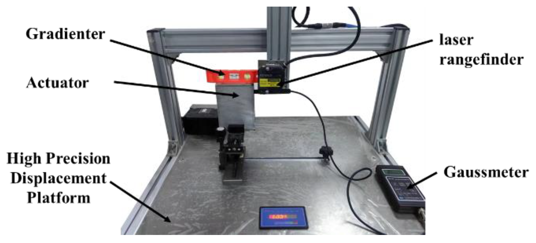
To validate the correctness of the analytical model for the non-uniform-size Halbach array’s magnetic flux density, an experimental platform for air-gap magnetic flux density measurements, as depicted in Figure 13, was designed. The platform consists of an actuator, a host computer, a 3-axis precision displacement stage, a KEYENCE LK-H057 laser sensor (Osaka, Japan), and a BST200H three-dimensional Gauss meter (Hangzhou, China). The Gauss meter integrates Hall probes, enabling the measurement of radial and tangential magnetic flux density. The permanent magnet array component of the actuator is fixed on the high-precision displacement platform, while the laser sensor and Gauss meter probes are mounted on the motion axes of the displacement platform in the x and z directions. The gaussmeter probe is in the center of the air gap of the Halbach array, and the gaussmeter probe is adjusted to the position of the magnetic flux density of the air gap by the KEYENCE LK-G5001P real-time position-controlled upscaling machine(Osaka, Japan). The intensity of the magnetic flux density in the z-direction on the centerline is measured.
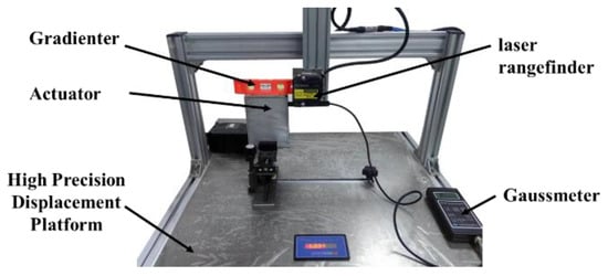
Figure 13.
Experimental platform for magnetic flux density measurement.
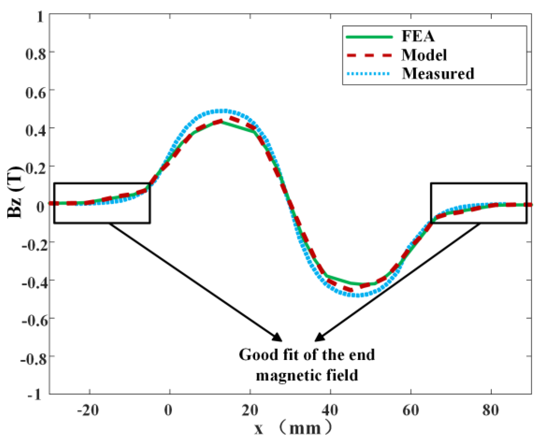
Using ANSYS finite element analysis software Maxwell 2016 the magnetic flux density of the actuator was analyzed. Within the operational stroke of the actuator coil, the effective air-gap magnetic flux density, i.e., the magnetic flux density in the vertical direction (z-axis), was measured. A comparison and analysis were conducted between the experimental measurement results and the numerical simulation results, as illustrated in Figure 14. From the experimental results shown in Figure 14, it can be observed that the z-direction magnetic flux density along the horizontal line at the center of the air gap is in good agreement with the finite element results. This demonstrates the reliability and accuracy of the analytical method to calculate the magnetic flux density produced by Halbach arrays.
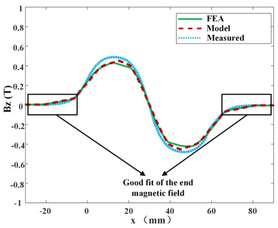
Figure 14.
Comparison of simulated and experimental values of air-gap magnetic flux density of permanent magnets.
3.2. Maglev Actuator Output Performance Test
The performance testing system of the magnetic levitation actuator is depicted in Figure 15, comprising a signal generator (B&K 3160-A-042, Hørning, Denmark), power amplifier (HEA-500G, Nanjing, China), accelerometer sensor, data acquisition card, and computer. The signal generator generates a sinusoidal waveform signal with adjustable frequency and magnitude. This signal is then amplified by the power amplifier and delivered to the coil. The accelerometer sensor measures the vibration signal of the mover and outputs it to the data acquisition card. The computer retrieves the data from the data acquisition card via serial communication. Therefore, a multimeter is connected between the power amplifier and the coil to measure the current in the coil.
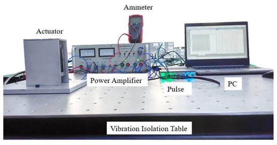
Figure 15.
Magnetic levitation actuator performance test methods.
The testing procedures primarily include the characterization of the force amplitude–frequency response and the assessment of force linearity within the magnetic levitation actuator.
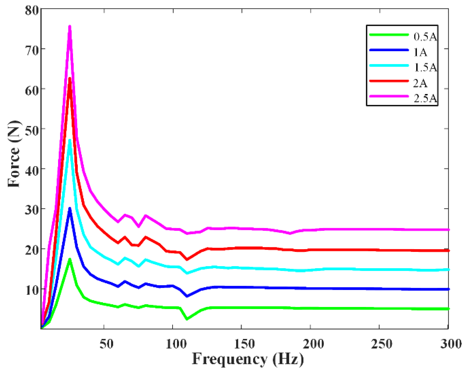
Force Amplitude–Frequency Response Test: This test involves investigating the relationship between the actuator’s acceleration and the frequency of the applied current. By analyzing the acceleration variation with respect to the current frequency and considering theoretical insights, the resonant frequency range of the mover can be determined.
The trends of the acceleration of the inertial mass portion of the magnetic levitation actuator corresponding to different current amplitudes (0.5 A, 1 A, 1.5 A, 2 A, and 2.5 A) as a function of current frequency are illustrated in Figure 16. It can be observed that around a frequency of approximately 20 Hz, the vibration acceleration response is maximized, indicating resonance in proximity to this frequency.
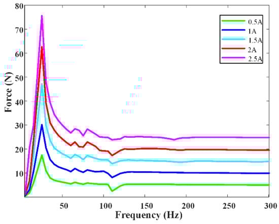
Figure 16.
Amplitude–frequency characteristic curve of the output force of the maglev actuator.
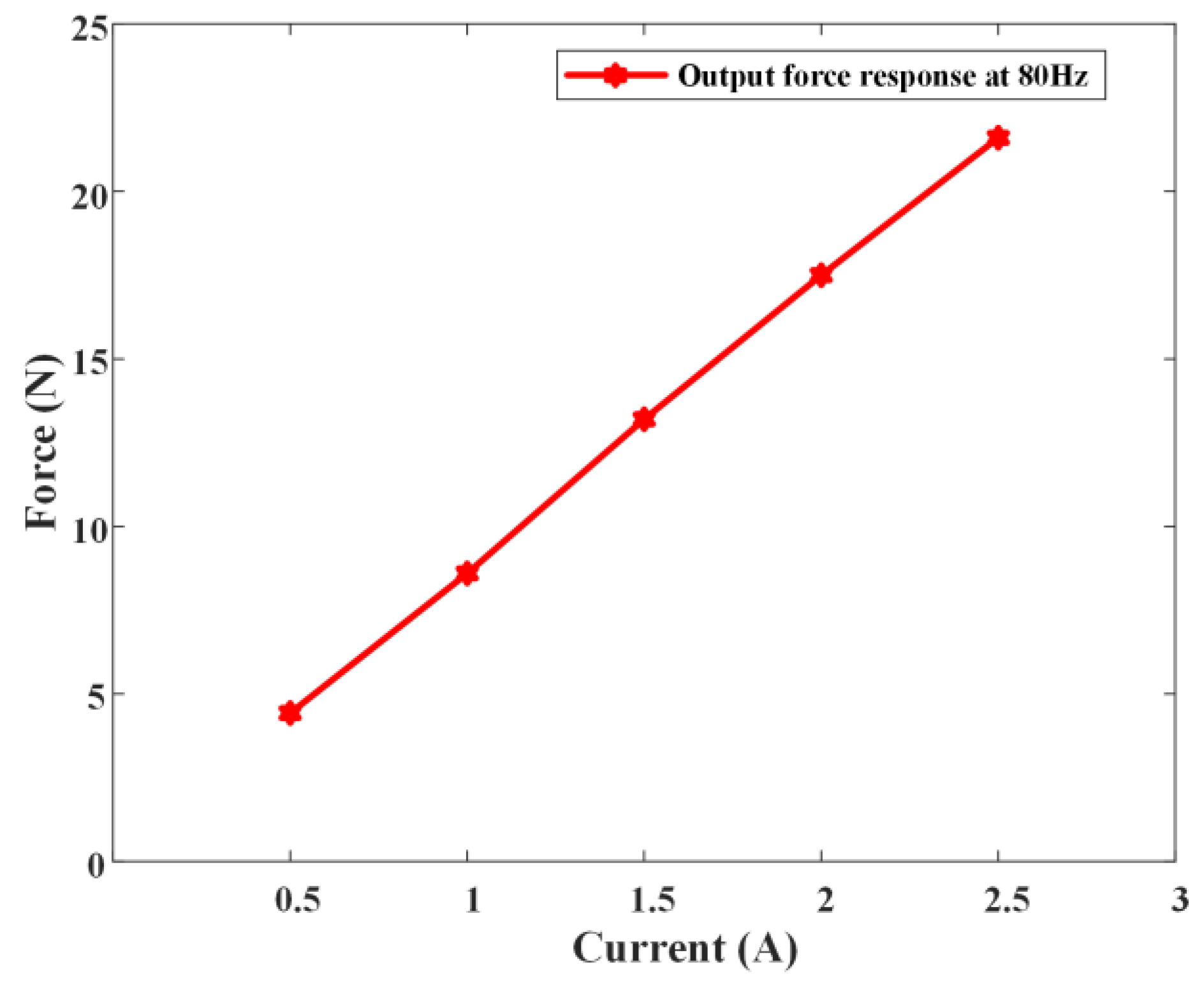
Force Linearity Test: The force characteristics serve as crucial performance parameters for the magnetic levitation actuator, where their linearity significantly influences the actual control effectiveness. Within the stable operational range of the magnetic levitation actuator (at 85 Hz current), the response of acceleration to the magnitude of current is depicted in Figure 17.
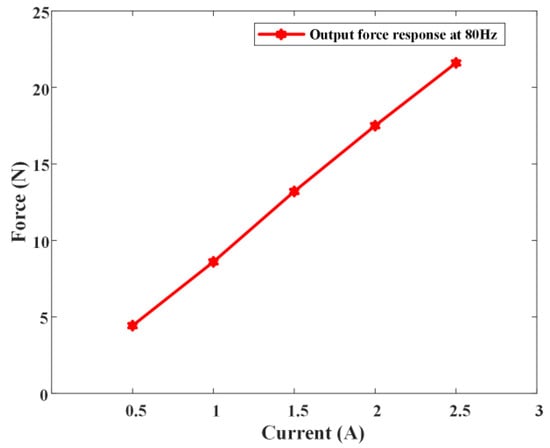
Figure 17.
Response curve of acceleration of maglev actuator with current at constant frequency.
It can be observed from Figure 17 that there exists a favorable linearity between the mover’s acceleration and the current, indicating conducive controllability of the output force of the magnetic levitation actuator.
4. Conclusions
This paper proposes a magnetic field analytical model based on the pseudo-periodic model of the permanent magnet array to address the distortion phenomenon caused by end effects. By redefining the mechanical pseudo-period, it resolves the challenge of difficult-to-solve end-field distortions caused by end effects. Furthermore, by introducing permanent magnets with different magnetization directions, it tackles the issue of incomplete pole pitch within one period, thereby obtaining a comprehensive analytical model of the magnetic field in the entire space, including the leakage field at the ends of the Halbach array. This study establishes non-uniform-size Halbach array magnetic field analytical mathematical models considering end effects and neglecting end effects. Using this analytical model, the magnetic flux density in the air gap of the magnetic levitation actuator can be calculated. Comparative analysis with Maxwell finite element simulation results validates the accuracy of the proposed model. Ultimately, it concludes that the analytical model considering end effects, established using Fourier analysis, is more accurate than the face current method. This model enhances the precision of the magnetic field model of the magnetic levitation actuator and lays the theoretical foundation for active control of shaft system vibrations, thus holding theoretical significance and engineering application value in enriching and developing control methods for fully electric integrated power systems.
Author Contributions
Conceptualization, Q.W. and Y.C. methodology, Y.C. software, Y.C. validation, Q.W., F.A. and B.L. formal analysis, Q.W. investigation, Y.C. resources, Q.W. data curation, Q.W. and G.Y. writing—original draft preparation, Q.W. and Y.C. writing—review and editing, F.A. and B.L. visualization, F.A. supervision, B.L. project administration, Q.W. funding acquisition, Q.W. All authors have read and agreed to the published version of the manuscript.
Funding
This research was funded by The Support plan for Outstanding Youth Innovation Team in Universities of Shandong Province (Grant No. 2022KJ165), the National Natural Science Foundation of China (Grant No. 51905288), the Taishan Scholar Program of Shandong (Grant No. ts201712054) and the Open Project of Key Laboratory of Industrial Fluid Energy Conservation and Pollution Control, Ministry of Education.
Data Availability Statement
The data presented in this study are available upon request from the corresponding author.
Conflicts of Interest
The authors declare no conflicts of interest.
References
- Smith, T.A.; La Rosa, A.G.; Wood, B. Underwater radiated noise from small craft in shallow water: Effects of speed and running attitude. Ocean Eng. 2024, 306, 118040. [Google Scholar] [CrossRef]
- Hong, D.K.; Park, J.H. Electromagnetic Design and Analysis of Inertial Mass Linear Actuator for Active Vibration Isolation System. Actuators 2023, 12, 295. [Google Scholar] [CrossRef]
- Volle, N.; Blanchet, A.; Goujard, B.; Valeau, V.; Sakout, A. Evaluation of Acoustic Comfort aboard Ships: An Investigation based on a Questionnaire. Electron. Des. Eng. 2003, 40, 2341–2347. [Google Scholar]
- Xie, X.; Qin, H.; Xu, Y.; Zhang, Z. Lateral vibration transmission suppression of a shaft-hull system with active stern support. Ocean Eng. 2019, 172, 501–510. [Google Scholar] [CrossRef]
- Blümler, P.; Soltner, H. Practical Concepts for Design, Construction and Application of Halbach Magnets in Magnetic Resonance. Appl. Magn. Reson. 2023, 54, 1701–1739. [Google Scholar] [CrossRef]
- Zhang, W.; Zhang, H.; Mu, J.; Wang, S. Design of a Single-Sided, Coreless, Flat-Type Linear Voice Coil Motor. Actuators 2023, 12, 77. [Google Scholar] [CrossRef]
- Hu, L.; Liu, M.; Yang, D.; Su, R.; Ruan, X.; Fu, X.; Li, Y. Calculation of field and force of Halbach arrays: Improved magnetic charge method for irregular magnetized magnets. Proc. Inst. Mech. Eng. Part C J. Mech. Eng. Sci. 2022, 236, 11136–11149. [Google Scholar] [CrossRef]
- Chen, Y.; Zhang, K. Analytical calculation of the spatial magnetic field of Halbach permanent magnet arrays. Magn. Mater. Devices 2014, 45, 1–4. [Google Scholar]
- Liu, R. Research on Permanent Magnet Motor Performance Analysis Method Based on Electromagnetic Field Numerical Calculation; Southeast University: Nanjing, China, 2002; pp. 30–54. [Google Scholar]
- Meng, G.; Li, H. Analytical calculation for air gap flux density of multi-pole permanent magnetic brushless DC motor. Trans. China Electrotech. Soc. 2011, 26, 37–42. [Google Scholar]
- Wuerkaixi, A.; He, S.; Wang, W.; Yu, J. Electromagnetic Field Analysis of High Capacity Permanent Magnet Wind Power Generator Based on Halbach Array. Electr. Mach. Control. Appl. 2016, 43, 68–72. [Google Scholar]
- Liu, G.; Zhang, H.; Ming, W. Application of trapezoidal magnets in Halbach magnet arrays for magnetically levitated planar motors. Electromech. Eng. Technol. 2018, 47, 105–108+157. [Google Scholar]
- Liu, K.; Chen, F.; Zhao, S.; Zhang, H.; Hu, A.; Wu, Y.; Zeng, L. Optimization of acceleration and force ripple of planar motor based a chamfered magnet array considering coil end effect. Sens. Actuators A Phys. 2024, 369, 115119. [Google Scholar] [CrossRef]
- Zhang, X.; Luo, H.; Sun, Y.; Hu, J.; Yang, Z. Analytical analysis of magnetic field and parametric design of moving-coil magnetically levitated permanent magnet planar motor. J. Sichuan Univ. Eng. Sci. Ed. 2015, 47, 142–150. [Google Scholar]
- Ham, C.; Ko, W.; Lin, K.C.; Joo, Y. Study of a hybrid magnet array for an electrodynamic maglev control. J. Magn. 2013, 18, 370–374. [Google Scholar] [CrossRef]
- Furlani, E.P. Permanent Magnet and Electromechanical Devices: Materials Analysis and Applications; Academic Press: New York, NY, USA, 2001. [Google Scholar]
- Jiang, Y.; Deng, Y.; Zhu, P.; Yang, M.; Zhou, F. Optimization on size of Halbach array permanent magnets for magnetic levitation system for permanent magnet Maglev train. IEEE Access 2021, 9, 44989–45000. [Google Scholar] [CrossRef]
- Wang, J.; Li, C.; Li, Y.; Yan, L. Optimization Design of Linear Halbach Array. In Proceedings of the 2008 International Conference on Electrical Machines and Systems, Wuhan, China, 17–20 October 2008; pp. 170–174. [Google Scholar]
- Song, Y.; Zhang, M.; Zhu, Y. Three-dimensional magnetic field end-effect modeling for Halbach permanent magnet array based on pseudo periodic. J. Electrotechnol. 2015, 30, 162–170. [Google Scholar]
- Li, X.; Cui, H.; Hu, C. Optimal design of thrust characteristics of flat-type permanent magnet linear synchronous motor. Trans. China Electrotech. Soc. 2021, 36, 916–923. [Google Scholar]
- Li, J.; Wu, X.; Chen, C. Analytical calculation of air gap magnetic field for permanent magnet machines based on pole partition processing. Proc. CSEE 2021, 41, 6390–6399. [Google Scholar]
- Jin, J.; Wang, X.; Zhao, C.; Xu, F.; Pei, W.; Liu, Y.; Sun, F. Characteristics Analysis of an Electromagnetic Actuator for Magnetic Levitation Transportation. Actuators 2022, 11, 377. [Google Scholar] [CrossRef]
- Jiang, X.; Wang, N.; Jin, M.; Zheng, J.; Pan, J. Vibration and force properties of an actuator formed from a piezoelectric stack within a frame structure. Sens. Actuators A Phys. 2024, 369, 115161. [Google Scholar] [CrossRef]
- Sun, Z.; Jia, G.; Huang, C.; Zhou, W.; Mao, Y.; Lei, Z. Accurate Modeling and Optimization of Electromagnetic Forces in an Ironless Halbach-Type Permanent Magnet Synchronous Linear Motor. Energies 2023, 16, 5785. [Google Scholar] [CrossRef]
- Kim, W. High-Precision Planar Magnetic Levitation. Ph.D. Thesis, Massachusetts Institute of Technology, Cambridge, MA, USA, 1997. [Google Scholar]
- Deng, C.; Liu, P. Analytical analysis of magnetic field of Halbach array voice coil motor based on method of sheet current. Micromotors 2018, 51, 7–11. [Google Scholar]


Disclaimer/Publisher’s Note: The statements, opinions and data contained in all publications are solely those of the individual author(s) and contributor(s) and not of MDPI and/or the editor(s). MDPI and/or the editor(s) disclaim responsibility for any injury to people or property resulting from any ideas, methods, instructions or products referred to in the content. |
© 2024 by the authors. Licensee MDPI, Basel, Switzerland. This article is an open access article distributed under the terms and conditions of the Creative Commons Attribution (CC BY) license (https://creativecommons.org/licenses/by/4.0/).