A Mechanical Fault Diagnosis Method for UCG-Type On-Load Tap Changers in Converter Transformers Based on Multi-Feature Fusion

Abstract

The On-Load Tap Changer (OLTC) is the only movable mechanical component in a converter transformer. To ensure the reliable operation of the OLTC and to promptly detect mechanical faults in OLTCs to prevent them from developing into electrical faults, this paper proposes a fault diagnosis method for OLTCs based on a combination of Particle Swarm Optimization (PSO) algorithm and Least Squares Support Vector Machine (LSSVM) with multi-feature fusion. Firstly, a multi-feature extraction method based on time/frequency domain statistics, synchrosqueezed wavelet transform, singular value decomposition, and multi-scale modal decomposition is proposed. Meanwhile, the random forest algorithm is used to screen features to eliminate the influence of redundant features on the accuracy of fault diagnosis. Secondly, the PSO algorithm is introduced to optimize the hyperparameters of LSSVM to obtain optimal parameters, thereby constructing an optimal LSSVM fault diagnosis model. Finally, different types of feature combinations are utilized for fault diagnosis, and the impact of these feature combinations on the fault diagnosis results is compared. Experimental results indicate that features of different types can complement each other, making the OLTC state information carried by multi-dimensional features more comprehensive, which helps to improve the accuracy of fault diagnosis. Compared with four traditional fault diagnosis methods, the proposed method performs better in fault diagnosis accuracy, achieving the highest accuracy of 98.58%, which can help to detect mechanical faults in the OLTC early and reduce the system’s downtime.

1. Introduction

The On-Load Tap Changer (OLTC) is the only movable mechanical component in a converter transformer [1]. It simultaneously endures electrical and mechanical stress, making it one of the most vulnerable components in the converter transformer [2]. Relevant data indicate that OLTC failures account for more than 20% of the total transformer failures, with mechanical failures constituting over 95% of all OLTC failures [3,4]. Therefore, it is of great significance to carry out research on an OLTC mechanical fault diagnosis technology of converter transformer and identify the hidden dangers of OLTC faults as early as possible to maintain the stable operation of high-voltage DC transmission systems.

The mechanical vibration signals of OLTCs carry abundant information about the state of the OLTC. In 1996, Bengtsson first introduced vibration signal analysis techniques into the OLTC mechanical fault diagnosis [5]. The core concept of this method is to use vibration sensors to monitor the vibration signals generated during the operation of the OLTC in a non-intrusive way, thereby obtaining OLTC state information for OLTC operation evaluation and judgment.

Currently, most of studies on OLTC mechanical fault diagnosis focus on rotary-type OLTCs [1,6,7], while studies on swing-arm-type OLTCs remain relatively scarce [7]. OLTC mechanical fault diagnosis methods can be roughly divided into two categories: one is to realize fault diagnosis through manual feature extraction combined with classifiers; the other is to use deep learning models for automatic feature extraction and fault diagnosis.

The manual feature extraction methods for OLTCs include time-domain feature extraction, frequency-domain feature extraction, time-frequency feature extraction, and dynamic feature extraction. These approaches have been extensively investigated by many researchers. Kang et al. employed continuous wavelet transform to extract time-domain envelope lines and successfully identified typical faults such as contact aging, erosion, and looseness using “ridge distribution maps” as features [8,9]. Gao et al. combined empirical mode decomposition with energy entropy to successfully distinguish between normal states and contact erosion faults [10]. Zhang et al. designed a time-frequency matrix partitioning algorithm and extracted parameter features such as partition lines, kurtosis, and envelope spectrum entropy [11]. Qian et al. utilized variational mode decomposition to extract the energy features of OLTC vibrations [12]. Zhao et al. utilized phase space reconstruction techniques to map one-dimensional time series signals into high-dimensional space and defined the phase point space distribution coefficient as the feature [13]. However, the existing methods have certain limitations. For instance, wavelet transform relies on extensive experience and expertise [14], while empirical mode decomposition is prone to mode mixing and endpoint effects [15]. The effectiveness of variational mode decomposition is significantly influenced by the number of decomposition components and the penalty factor [16]. Meanwhile, phase space reconstruction methods are sensitive to noise and computationally intensive [17]. In OLTC fault diagnosis, commonly used classifiers include Support Vector Machine (SVM) [1], BP neural network [18], Long Short-Term Memory network (LSTM) [19], and Convolutional Neural Network (CNN) [20].

There are two main methods of applying deep learning-based automatic feature extraction in OLTC fault diagnosis. The first method directly employs the neural networks to process the OLTC vibration signals and uses the hierarchical structure of the network to automatically extract signal features to perform fault diagnosis [21]. The second method is to convert the OLTC vibration signals into images, and then extract key features from the image through deep learning methods such as CNNs to achieve fault diagnosis [22,23].

Deep learning models can automatically extract features from OLTC vibration signals, eliminating the need for complex preprocessing and feature engineering, and significantly simplifying the feature design process [24,25]. These models also exhibit strong generalization capabilities [26]. For instance, target transfer deep learning methods based on a distribution barycenter medium [27], along with label recovery and trajectory-designable deep transfer learning methods [28], can effectively achieve fault diagnosis between different devices of the same type. However, they often struggle to explain the specific relationships between features and faults [26]. Additionally, deep learning models typically require large amounts of labeled data for training, they are prone to overfitting or reduced diagnostic accuracy when training data are insufficient [29]. Moreover, due to their complex network structures, deep learning models consume significant computational resources and have long training times, making them unsuitable for real-time or resource-constrained applications [30].

Manual feature extraction relies on domain knowledge, with clear correspondence between features and actual physical phenomena, making the diagnostic results easier to interpret [31]. The extracted features are typically of lower dimensionality, consuming fewer computational resources, which is well-suited for real-time applications [32]. In cases where the data sample size is limited, the fault diagnosis methods based on the manual feature extraction often perform more consistently than deep learning models based on small datasets [33].

In practical operations, OLTC faults occur infrequently, making it a typical small-sample-size diagnostic problem. The Least Squares Support Vector Machine (LSSVM), with its high accuracy, fast training speed, simple parameter tuning, excellent small-sample handling capability, and outstanding nonlinear processing ability, has emerged as a powerful tool for addressing the difficulties in fault diagnosis [34]. However, in the LSSVM model, the penalty factor c and the kernel parameter g have a significant impact on the model performance, so these hyperparameters need to be optimized.

As an intelligent optimization algorithm, Particle Swarm Optimization (PSO) has the characteristics of few parameters, fast calculation speed, and strong global search ability [35]. Therefore, this study employed PSO to optimize the hyperparameters of LSSVM. To prevent PSO from falling into a local optimum, PSO was used to optimize the hyperparameters multiple times, so as to obtain the optimal hyperparameters of LSSVM.

This paper focuses on the UCG-type OLTC used in high-voltage DC converter transformers. The UCG-type OLTC employs a swing-arm switching mechanism, which differs from the rotary-type OLTC [6,7]. The vibration signals generated by these two types of OLTCs during the operation exhibit significant differences. Consequently, a multi-feature extraction method is proposed to address the issue of the low accuracy of fault diagnosis based on a single feature. Additionally, a PSO-LSSVM-based fault diagnosis model is developed to achieve accurate diagnosis of OLTCs’ mechanical faults. Firstly, vibration signals under different OLTC fault conditions are collected through the experimental test platform, and time-domain and frequency-domain statistical features, singular-value features of time-frequency matrices, and multi-scale modal features are extracted. Secondly, multi-dimensional feature vectors are constructed, and the random forest algorithm is employed for feature selection to eliminate the influence of redundant features, thereby improving the accuracy and reliability of fault diagnosis. Finally, PSO is applied to optimize the penalty factor c and kernel parameter g of the LSSVM model, and a PSO-LSSVM fault diagnosis model is built.

The results demonstrate that the multi-feature extraction method can effectively capture the feature changes of OLTCs under different states, while the LSSVM model optimized by the PSO can accurately identify mechanical faults in OLTCs. This study provides an effective method for diagnosing mechanical faults in high-voltage DC converter transformer OLTCs, preventing early mechanical faults in OLTCs from evolving into electrical faults.

The contributions of this paper are listed as follows:

(1)

This paper focuses on the mechanical fault diagnosis of swing-arm-type (UCG-type) OLTCs, which are employed in 800 kV high-voltage DC converter transformers.

(2)

A multi-feature extraction method is proposed, which overcomes the shortcomings of insufficient information of a single feature, which leads to a low accuracy of fault diagnosis.

(3)

The feature importance evaluation based on random forest algorithm is introduced to screen the features and eliminate redundant features, so as to find the most effective feature combination, which can further improve the accuracy of fault diagnosis.

(4)

The parameters of LSSVM are optimized by the PSO algorithm, and a small-sample-size fault diagnosis model based on PSO-LSSVM is established, and then the model is applied to the fault diagnosis of a UCG-type OLTC; good fault diagnosis results are obtained.

2. Proposed Mechanical Fault Diagnosis Method

This study extracts multi-dimensional features of OLTC vibration signals from four perspectives: time-domain features, frequency-domain features, time-frequency matrix energy features, and multi-scale modal features. A PSO-optimized LSSVM model is then utilized for fault diagnosis. The specific process of the proposed method is illustrated in Figure 1, with the main steps as follows:

(1)

Step I: An experimental test platform for the UCG-type converter transformer OLTC is constructed. Multiple vibration sensors are used to collect OLTC vibration signals under different states.

(2)

Step II: Multi-dimensional feature extraction is performed on the collected OLTC vibration signals, creating a dataset of features. The random forest algorithm is used to screen the features to eliminate the influence of any redundant features.

(3)

Step III: An OLTC fault diagnosis model based on PSO-optimized LSSVM is established. The detailed optimization process is discussed in Section 4.2. Firstly, the number of PSO optimization iterations is preset. After each iteration, an optimal combination of hyperparameters is obtained and it is used to conduct 20 fault diagnosis tests. Consequently, the average optimal accuracy rate is calculated. Then, the optimization LSSVM model is obtained by synthesizing the results of multiple optimizations and selecting the hyperparameters corresponding to the optimal accuracy. Finally, the optimal LSSVM model is employed for OLTC mechanical fault diagnosis, yielding the diagnostic results.

3. OLTC Vibration Signal Acquisition

In this study, the UCG-type OLTC manufactured by Hitachi Energy was used to build the experimental test platform. The tests were conducted under no-load conditions. The UCG-type OLTC consists of a motor drive unit, a diverter switch, and a selector switch, which is illustrated in Figure 2. The switching process of the UCG-type OLTC follows the sequence in which the selector switch first selects, and then the diverter switch operates.

The sensor adopts Beijing QUATRONIX ULT2001 piezoelectric vibration sensor (QUATRONIX Electronics Co., Ltd., Beijing, China) with a range of ±50 g and a sensitivity of 100 mV/g, and the frequency response range is 0.5~15 kHz. A data acquisition card with a sampling frequency of up to 100 kHz is employed. The data acquisition process is illustrated in Figure 3.

The installation position of the vibration sensors is shown in Figure 4, in which four vibration sensors are installed on the top of the OLTC.

Figure 5 illustrates the setting of four fault conditions. In Figure 5a, the fault of the upper stationary contact loosening is set by loosening the screws of the upper stationary contact. In Figure 5b, the fault of the lower stationary contact loosening is set by loosening the screws of the lower stationary contact. In Figure 5c, the fault of the insulation plate loosening is set by loosening the screws of the insulation plate. In Figure 5d, the fault of the moving contact loosening is set by cutting the spring that connects the moving contact. Data from five conditions were collected, including normal, upper stationary contact loosening, lower stationary contact loosening, insulation plate loosening, and moving contact loosening conditions.

The UCG-type OLTC vibration signals under different operating conditions are shown in Figure 6. By comparing Figure 6c,e,g,i with Figure 6a, it can be observed that when different types of loosening faults occur, the vibration signal intensity in the time domain changes, and the waveform shows significant differences. A comparison of Figure 6d,f,h with Figure 6a reveals that in the frequency domain, when the upper static contact, lower static contact, or insulation plate become loose, a significant number of low-frequency components appears in the vibration signal. When the moving contact becomes loose, both high-frequency and low-frequency components increase. Compared to normal conditions, the peak value of the vibration intensity decreases. Therefore, the mechanical fault diagnosis of the UCG-type OLTC can be achieved by extracting the frequency distribution characteristics of the UCG-type OLTC vibration signals.

4. Multi-Feature Extraction Method for OLTC Vibration Signals

To obtain the feature variations of OLTC vibration signals under different operating conditions, this study extracted both time-domain and frequency-domain features of the OLTC vibration signals, focusing on the overall changes in the vibration signals. By employing synchrosqueezed wavelet transform (SWT), detailed features of the time-frequency energy distribution were extracted. The multi-scale decomposition of the signals was performed to focus on the local features. The complementary nature of different feature types enhances the accuracy of fault diagnosis.

4.1. Statistical Feature Extraction in the Time/Frequency Domain

OLTC vibration signals typically manifest in the form of impulse waves. When a fault occurs in the OLTC, the statistical features of the vibration signal in both the time and frequency domains will change due to the change of fault type and fault severity, which can be used as the basis for fault diagnosis. When a fault occurs in the OLTC, the amplitude and the distribution of vibrational energy change in the time-domain, while the signal frequency and energy distribution also change in the time-domain.

Table 1. Time-domain statistical features [36].

Feature	Calculation Formula	Feature	Calculation Formula
Mean	$S_1={\displaystyle \frac{1}{N}}{\displaystyle \sum _{i=1}^N\left|x(n)\right|}$	Crest Factor	$S_5=S_4/S_3$
Root Amplitude	$S_2={\left({\displaystyle \frac{1}{N}}{\displaystyle \sum _{i=1}^N\sqrt{\left|x(n)\right|}}\right)}^2$	Form Factor	$S_6=S_3/S_1$
Root Mean Square	$S_3=\sqrt{{\displaystyle \frac{1}{N}}{\displaystyle \sum _{i=1}^N{x}_i^2}}$	Impulse Factor	$S_7=S_4/S_1$
Peak-to-Peak Value	$S_4=\max (x_i)-\min (x_i)$	Margin Indicator	$S_8=S_4/S_2$

shows the calculation methods for time-domain features, while

Table 2. Frequency-domain feature parameters [36].

Feature	Calculation Formula	Feature	Calculation Formula
Average Energy	$P_1={\displaystyle \sum _{i=1}^N{X}_{\mathrm{i}}}/N$	Frequency Standard Deviation	$P_3=\sqrt{{\displaystyle \sum _{i=1}^K{(f_i-P_2)}^2\times X_i}/{\displaystyle \sum _{i=1}^N{X}_i}}$
Central Frequency	$P_2={\displaystyle \sum _{i=1}^N(f_i\times X_i)}/{\displaystyle \sum _{i=1}^N{X}_i}$	Dispersion Factor	$P_4={\displaystyle \sum _{i=1}^N{(X_i-P_2)}^3}/{\displaystyle \sum _{i=1}^N{X}_{\mathrm{i}}}\times {(P_2)}^{{\displaystyle \frac{3}{2}}}$

illustrates the calculation methods for frequency-domain features. In these two tables, x_i represents the raw OLTC vibration signal, and N denotes the sampling length of the signal. X_i represents the frequency-domain signal of x_i, and f_i denotes the frequency values of each frequency-domain point.

4.2. Singular Value Feature Extraction of Time-Frequency Matrix

4.2.1. Synchrosqueezed Wavelet Transform

In 2011, Daubechies et al. proposed a synchronous compression transform method based on continuous wavelet transform, which is SWT [37]. This method enhances frequency aggregation and energy concentration by reordering the frequency series, thus achieving more efficient compression transformation. The formula for SWT is obtained from reference [37]. First, the continuous wavelet transform of the signal s(t) is expressed as

$$W_s^{\psi }(a,b)={\displaystyle \frac{1}{\sqrt{a}}}{\displaystyle {\int }_{-\infty }^{+\infty }s(t)\psi \left(\frac{t-b}{a}\right)}dt$$

(1)

where a is the scale factor, b is the translation factor, $\psi \left(t\right)$ is the wavelet basis function, and $\overline{\psi \left(t\right)}$ is the conjugate function of $\psi \left(t\right)$.

For any $W_s^{\psi }(a,b)\ne 0$ of (a, b), the instantaneous frequency ${\omega }_s(a,b)$ of the signal s(t) is given by the following equation:

$${\omega }_s(a,b)=-j{\displaystyle \frac{{\partial }_b{W}_s^{\psi }(a,b)}{W_s^{\psi }(a,b)}}$$

(2)

where ${\partial }_b{W}_s^{\psi }(a,b)$ is the partial derivative of the continuous wavelet transform $W_s^{\psi }(a,b)$ with respect to the translation factor b.

Based on the mapping relationship $(a,b)\to ({\omega }_s(a,b),b)$, in the time-frequency plane, the continuous wavelet transform coefficient $W_s^{\psi }(a,b)$ can be reordered using synchronous compression calculation as follows:

$$T_{\mathrm{s}}(\omega ,b)={\displaystyle {\int }_{-\infty }^{+\infty }{W}_s^{\psi }}(a,b)a^{-3/2}\delta [{\omega }_s(a,b)-\omega ]da$$

(3)

4.2.2. Singular Value Decomposition Feature Extraction

The singular values obtained by the Singular Value Decomposition (SVD) of the matrix contain important information of the matrix and are widely used for the feature extraction of signals [38]. For any given matrix M, there are orthogonal matrices U and V, and it can be decomposed as

$$M_{m\times n}=US{V}^T$$

(4)

$$S=diag({\sigma }_1,{\sigma }_{2,}\cdots ,{\sigma }_{r,}\cdots ,0)$$

(5)

where ${\sigma }_1,{\sigma }_{2,}\cdots ,{\sigma }_{r,}\cdots ,0$ are the singular values of the matrix M.

The time-frequency matrix of the OLTC vibration signal is obtained by SWT. Each element of this matrix is modulated, and then the SVD is performed. Therefore, the obtained singular values reflect the features of the OLTC vibration signal, and the corresponding feature matrix is determined. Since the number of singular values is affected by the number of rows and columns of the amplitude matrix, which is usually larger, further processing is required to highlight the relative changes in the OLTC vibration signal in different states. This paper extracts the maximum and average singular values of the OLTC vibration signal in different states as features, which are expressed as

$$T_1=\max ({\sigma }_1,{\sigma }_2,\cdots ,{\sigma }_r)$$

(6)

$$T_2={\displaystyle \frac{{\sigma }_1+{\sigma }_2+\cdots +{\sigma }_r}{r}}$$

(7)

4.3. Multi-Scale Mode Feature Extraction

To enhance the sensitivity to subtle changes in OLTC states, the Improved Complete Ensemble Empirical Mode Decomposition with Adaptive Noise (ICEEMDAN) is used to decompose the OLTC vibration signal [39]. ICEEMDAN is an improved signal decomposition method, which effectively solves the modal aliasing problem in the EEMD algorithm by introducing Gaussian white noise and redefining the modal mean, thereby significantly improving the accuracy and stability of signal decomposition [39]. The specific process is given as follows, the formula for ICEEMDAN is obtained from reference [39].

(1)

Step I: Add m sets of white noise ${\omega }^{(m)}$ to the original sequence x to obtain a new sequence, which is given by

$$X_1^{(m)}=x+B_1{E}_1({\omega }^{(m)})$$

(8)

where $B_k$ is the noise of the r-th sequence, and $E_k(\cdot )$ represents the k-th mode component of the EMD decomposition.

(2)

Step II: Calculate the first residual signal $r_1$ and mode component IMF₁, which are given by

$$r_1=〈X_1^{(m)}-E_1(X_1^{(m)})〉$$

(9)

$$IM{F}_1=x-r_1$$

(10)

where $M(\cdot )$ represents the local mean of the generated signal, and $〈\cdot 〉$ is the averaging operator.

(3)

Step III: Continue to add white noise to $r_1$, and then find the mean value to obtain ${X_2}^{(m)}=x+B_1{E}_1({\omega }^{(m)})$, and calculate the modal component IMF2 of the second set of residual signal $r_2$, which are given by

$$r_2=〈X_2^{(m)}-E_2(X_2^{(m)})〉$$

(11)

$$IM{F}_2=r_1-r_2$$

(12)

(4)

Step IV: Repeat Step III to obtain the k-th residual signal and the k-th mode component, which can be obtained by

$$r_k=〈X_k^{(m)}-E_k(X_k^{(m)})〉$$

(13)

$$IM{F}_k=r_{k-1}-r_k$$

(14)

(5)

Step V: Return to Step IV until the residual signal can no longer be decomposed or meets the stop criterion, obtaining all mode components.

After ICEEMDAN decomposition, the original signal is decomposed into multiple IMF components, each of which has a different correlation with the original signal. Therefore, the Pearson correlation coefficient method is used to screen out the first k modes IMF_k with higher correlation to the original signal, reducing the interference of irrelevant components. Then, the frequency-domain mean value M_IMF and the central frequency G_IMF of each IMF are extracted, and they are combined to form the multi-scale mode features. The specific calculation formulas can be expressed as

$$M_{IMF}={\displaystyle \sum _{k=1}^{N}IMF(k)}/N$$

(15)

$$G_{IMF}={\displaystyle \sum _{k=1}^{N}IMF(k)\times f_k}/{\displaystyle \sum _{k=1}^{N}IMF(k)}$$

(16)

where f_k is the frequency corresponding to each component spectrum, and N is the sample size of the IMF sequence.

4.4. Feature Screening Based on Random Forest Algorithm

The extracted UCG-type OLTC vibration signal features have high dimensionality, and there may be redundant features. By utilizing the random forest algorithm for feature screening, the impact of redundant features on the accuracy of fault diagnosis can be effectively avoided [40]. The random forest algorithm can evaluate the importance of features by measuring their contribution in each decision tree and averaging them. This allows for the features to be ranked and the influence of each feature to be compared [41].

4.4.1. Construction Principles of the Random Forest Algorithm

The construction process of the random forest model is shown in Figure 7. Suppose the dataset contains H samples, and each sample has M features. The specific process is given as follows:

(1)

Step I: Use the bootstrap method to randomly select 2H/3 of the samples from the dataset to create a training set.

(2)

Step II: Generate a decision tree for each training set. Randomly select M features (without repetition) as candidate features, and use these M features to determine the optimal feature that results in the best splitting effect.

(3)

Step III: Repeat step I and step II until k decision trees are generated.

(4)

Step IV: The trained random forest is used to make predictions on the testing set, and the final prediction result is determined by a voting mechanism.

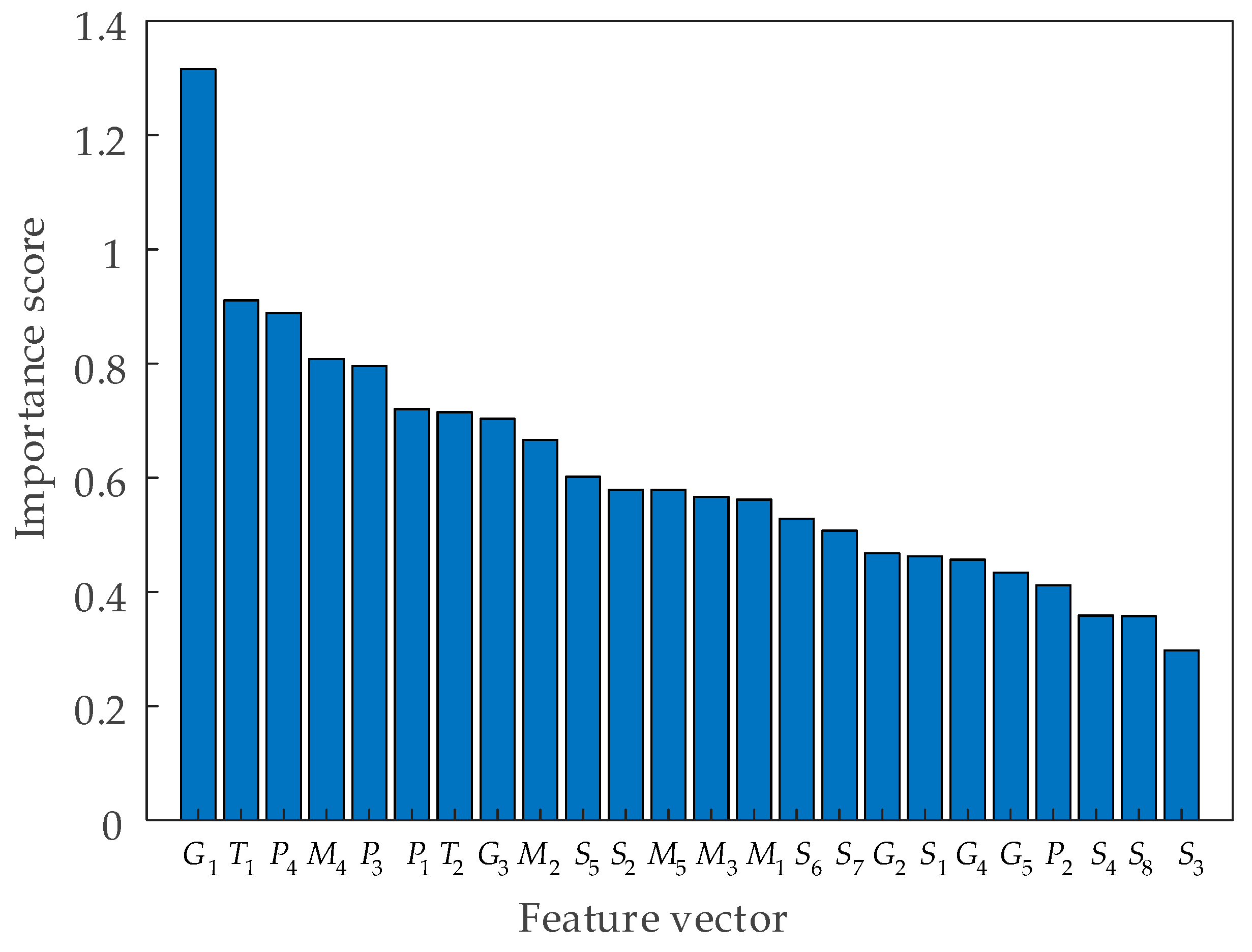
4.4.2. Feature Importance Evaluation

When the random forest algorithm is used to evaluate the feature importance, its core idea is to quantify the contribution of each feature to the model performance. In random forest algorithms, Out-Of-Bag (OOB) error is often used as an indicator to assess the contribution of each feature [41]. The Feature Importance Measure (FIM) reflects the contribution of each feature to the classification accuracy.

The $FI{M}_{km}^{(OOB)}$ of feature $F_m$ in the k-th decision tree is calculated as follows [41]:

$$FI{M}_{km}^{(OOB)}={\displaystyle \frac{{\displaystyle \sum _{p=1}^{n_0^k}I}(Y_p,Y_p^k)}{n_0^k}}-{\displaystyle \frac{{\displaystyle \sum _{p=1}^{n_0^k}I}(Y_p,Y_{p,\pi m}^k)}{n_o^k}}$$

(17)

where I(x,y) is an indicator function, which is defined as $I(x,y)=\left\{\begin{array}{c}1,x=y\\ 0,x\ne y\end{array}\right.$. It is used to determine whether the classification result is correct. $n_o^k$ is the number of OOB samples in the k-th decision tree, $Y_p$ is the true label of the p-th sample, and $Y_p^k$ is the predicted result of the p-th sample in the k-th decision tree without feature permutation. $Y_p^{k,m}$ is the predicted result of the p-th sample after feature $F_m$ has been permuted in the k-th decision tree.

By comparing the classification accuracy of OOB samples before and after permuting feature $F_m$, the contribution of the feature to the classification accuracy can be measured. If the classification accuracy decreases significantly after the permutation, it indicates that this feature plays a crucial role in the random forest algorithm.

To obtain the overall importance score of feature $F_m$ in the random forest, $FI{M}_{km}^{(OOB)}$ in k-th decision tree is averaged and divided by the standard deviation to reduce the uncertainty. It is calculated as follows [41]:

$$FI{M}_m^{(OOB)}={\displaystyle \frac{{\displaystyle \sum _{k=1}^{K}F}I{M}_{km}^{(OOB)}}{K\sigma }}$$

(18)

where K is the total number of trees in the random forest, and σ is the standard deviation of the importance score $FI{M}_{km}^{(OOB)}$ for feature $F_m$.

4.4.3. Feature Screening Process Based on the Random Forest Algorithm

The steps for feature screening using the random forest algorithm are given as follows:

(1)

Step I: Extract features from the UCG-type OLTC vibration signals.

(2)

Step II: Construct a random forest model.

(3)

Step III: Calculate the importance scores of the features.

(4)

Step IV: Based on the feature importance scores, screen features step by step according to the ranking from high to low.

5. PSO-LSSVM-Based OLTC Fault Diagnosis

5.1. LSSVM

The main difference between LSSVM and the traditional Support Vector Machine (SVM) lies in the modification of the objective function and the constraint conditions [42]. In traditional SVM, the optimization problem is a convex quadratic programming problem that includes inequality constraints; whereas in LSSVM, the optimization changes to a linear programming problem, which greatly simplifies the calculation process.

The formula for LSSVM is obtained from reference [42]. The optimization problem of LSSVM can be expressed as

$$\left\{\begin{array}{l}{\min }_{\omega ,b,e}J(\omega ,e)={\displaystyle \frac{1}{2}}{\omega }^T\omega +{\displaystyle \frac{c}{2}}{\displaystyle \sum _{i=1}^N{e}_u^2}\\ y_i={\omega }^T\varphi (h_u)+b+e_u\forall u=1,\cdots ,N\end{array}\right.$$

(19)

where $\omega$ is the weight vector, b is the bias, e is the error term, and c is the regularization parameter.

The optimization process of LSSVM is given as follows:

(1)

Step I: By introducing Lagrange multipliers ${\alpha }_i$, the optimization problem can be transformed into solving a linear programming problem, thereby improving the computational efficiency. The constructed Lagrange function is given by

$$L(\omega ,b,e,\alpha )={\displaystyle \frac{1}{2}}{\omega }^T\omega +{\displaystyle \frac{c}{2}}{\displaystyle \sum _{u=1}^N{e}_u^2}-{\displaystyle \sum _{u=1}^n{\alpha }_u\left[y_u-{\omega }^T\varphi (h_u)-b-e_u\right]}$$

(20)

(2)

Step II: Solve the Karush–Kuhn-Tucker (KKT) conditions. The KKT conditions can be obtained by taking derivatives of $\omega ,b,e,\alpha$ in Equation (20) and setting them to zero, which are given by

$$\left\{\begin{array}{l}\omega ={\displaystyle \sum _u^{.n}{\alpha }_u\varphi (h_u)}\\ {\displaystyle \sum _i^{.n}{\alpha }_u=0}\\ {\alpha }_u=c{e}_u\\ {\omega }^T\varphi (h_u)+b+e_u=y_u\end{array}\right.$$

(21)

(3)

Step III: Solve the system of linear equations. By expressing the linear equations in matrix form, the optimal $\omega$ and $b$ can be obtained using matrix operations.

5.2. PSO-Optimized LSSVM for OLTC Fault Diagnosis

The performance of LSSVM highly depends on the selection of hyperparameters, including the regularization parameter c and kernel parameter g. The predictive ability of the model will be affected if the parameters are not selected properly. In addition, manual tuning of these parameters is cumbersome and time-consuming, and it usually requires the use of methods such as grid search or random search. These methods are inefficient in the space of high-dimensional parameters. Moreover, the objective function of LSSVM is usually non-linear and non-convex, which is easy to fall into the local optimum, making it difficult for traditional optimization methods to find the global optimal solution.

This study employs PSO [35] to optimize the parameters of the LSSVM model. The fundamental principles of PSO-based optimization for LSSVM are given as follows:

(1)

Step I: Initialize the parameters of PSO. The search range for parameter c is set to [0.1, 300], and the search range for parameter g is set to [0.1, 10]. The optimization parameter dimension D is equal to 2, the maximum number of iterations is 20, and the particle swarm size N is equal to 5. The initial maximum velocity of the particle is set to 10, and its minimum velocity is set to -10. The formula for PSO is obtained from reference [43]. The initialization processes of the particle positions $Q_i$ and velocities $v_i$ are given as follows:

$$\left\{\begin{array}{l}{Q}_i=rand(N,D)•(L_{maxj}-L_{\min j})+L_{\min j}\\ v_i=rand(N,D)•(V_{max}-V_{min})+V_{min}\end{array}\right.$$

(22)

where rand(•) represents a random vector, $L_{\min j}$ and $L_{\max j}$ denote the lower and upper bounds of the problem, respectively. $Q_i$ represents the current position of the i-th particle, and the velocity $v_i$ indicates the direction and rate of position changes.

(2)

Step II: Calculate the initial fitness value. The dataset is divided into a training set and testing set in an 8:2 ratio. The current particle $Q_i$ is used to train the LSSVM model, and the classification accuracy of the training set is obtained. The fitness value of the particle is then calculated by using the classification error rate of the testing set, which is given by the following formula:

$$f(Q_i)=1-Accuracy$$

(23)

where Accuracy refers to the classification accuracy of the testing set.

(3)

Step III: Update the individual optimal position $p_{best,i}$ of the particle. Let the current position of the particle be $Q_i$, and its current fitness value be $f(Q_i)$. If $f(Q_i)<f(P_{best,i})$, then update $P_{best,i}=Q_i$.

(4)

Step IV: Update the global optimal position $G_{best}$ of the particle. For each generation, find the particle with the smallest $f(P_{best,i})$. The current global best fitness value of the particle is $f(P_{best,i})$. If the individual optimal position of any particle $f(P_{best,i})<f(G_{best})$, then the global optimal position is updated to $G_{best}=P_{best,i}$.

(5)

Step V: Update the position and velocity of the particle. The velocity update equation for the particle is given as follows [43]:

$$v_i(t+1)=\omega \cdot v_i(t)+c_1\cdot r_1\cdot (p_{best}-Q_i(t))+c_2\cdot r_2\cdot (p_{best}-Q_i(t))$$

(24)

The position update formula for the particle is given as follows [43]:

$$Q_i(t+1)=Q_i(t)+v_i(t+1)$$

(25)

where $r_1$ and $r_2$ are random numbers in the range of [0, 1], $c_1$ and $c_2$ are learning factors whose value is set to 1.5, and $\omega$ is the inertia weight, which is set to 0.8.

(6)

Step VI: Repeat steps (3) to (5). When the maximum number of iterations or other stopping criteria are met, the optimal combination of parameters c and g are obtained.

When the PSO algorithm is applied, PSO might fall into local optima during the single optimization process. This paper proposes a method to improve the process of PSO-optimized LSSVM. After each optimization, multiple fault diagnoses are performed using the optimized LSSVM to further determine whether the optimized parameters make the model perform the best. The optimal combination of c and g is obtained by combining the results of multiple optimizations, which can not only make full use of the global search ability of PSO, but also avoid PSO from falling into local optimization in a single optimization. Consequently, the optimal hyperparameters of LSSVM can be found by the improved optimization method. The flowchart of the improved optimization method is given in Figure 8, which includes four main steps as follows:

(1)

Step I: Setting the number of optimizations.

(2)

Step II: Optimizing the regularization parameter c and kernel parameter g of LSSVM using PSO to obtain the optimal parameter combination for each optimization.

(3)

Step III: Using the optimized LSSVM parameters to perform 20 training and testing iterations, calculating and recording the average accuracy of the test set.

(4)

Step IV: To avoid PSO falling into local optima, the parameter combination with the highest average accuracy of LSSVM is found by the multiple optimizations, and the optimal LSSVM model is obtained.

6. Experiment and Result Analysis

6.1. Pre-Processing of OLTC Vibration Signals

During normal operation, the OLTC performs a typical tap position change (from the tap position 20 to 19), the vibration signals collected by different measurement points are shown in Figure 9. It can be seen that the vibration amplitudes of different positions are quite different. Among them, the amplitudes of measurement points #1 and #3 are similar, and the amplitudes of measurement points #2 and #4 are similar. Since measuring point #3 is closest to the OLTC actuator and is more sensitive to the change of the OLTC’s mechanical state, the vibration signal of measuring point #3 is mainly used in the subsequent analysis.

To eliminate the dimensional differences between different signals and reduce the data instability, a normalization process is adopted, which is given by

$$Z_i={\displaystyle \frac{x_i-\mu }{\sigma }}$$

(26)

where $x_i$ is the original signal, $\mu$ is the mean value of the original signal, $\sigma$ is the standard deviation of the original signal, and $Z_i$ is the result after normalization.

6.2. Comparative Analysis of Different Feature Combinations

To more intuitively compare the advantages of the multi-dimensional feature fusion method over single-dimensional features, this paper combines different types of features and calculates the average accuracy of 20 fault diagnosis iterations under different combinations. The results are tabulated in

Table 3. Comparison of the average accuracy of the training set and the test set composed of different feature combinations.

Feature Name	Average Training Accuracy	Average Testing Accuracy
Time/Frequency Domain	94.98 ± 3.21%	90.11 ± 5.19%
SWT-SVD	75.53 ± 3.58%	71.72 ± 6.72%
Multi-Scale Modal Features	97.85 ± 2.25%	90.69 ± 4.71%
Time/Frequency Domain + SWT-SVD	98.71 ± 0.65%	92.35 ± 3.84%
Time/Frequency Domain + Multi-Scale Modal Features	99.22 ± 0.28%	94.01 ± 3.25%
SWT-SVD + Multi-Scale Modal Features	99.18 ± 0.35%	95.23 ± 3.57%
Time/Frequency Domain + SWT-SVD+ Multi-Scale Modal Features	100.00 ± 0.00%	97.98 ± 2.14%

. From Table 3, it can be seen that the performance of single features is quite limited. Different types of features contain various types of fault information and can complement each other. By using multi-feature fusion for fault diagnosis, the accuracy of fault diagnosis can be significantly improved.

6.3. Feature Analysis Based on Random Forest Algorithm

Using the multi-feature extraction method presented in Section 4, the time-domain features $S_1~S_8$, frequency-domain features $P_1~P_4$, singular-value features of the time-frequency matrix $T_1~T_2$, multi-scale modal frequency-domain energy features $M_1~M_5$, and multi-scale modal center of gravity frequency $G_1~G_5$ are obtained, and a total of 24-dimensional features are extracted. These features may contain some redundant features. Therefore, the random forest algorithm is used to screen out features with high sensitivity to faults, and redundant features are eliminated to improve the accuracy of fault diagnosis.

The dataset was divided into a training set and a testing set with a ratio of 8:2. The training set was used to train a random forest model. After training, feature importance scores were calculated for each feature. The importance scores of each feature calculated by the random forest algorithm are shown in Figure 10. The higher the score, the greater the role of the feature in the model. According to the order of the important score, the selected features were combined, and the LSSVM was used for fault diagnosis. The average accuracy rate of 20 repeated tests was calculated and is shown in Figure 11.

From Figure 10, it can be seen that the importance scores of each feature calculated by the random forest algorithm were all above 0.2. Using the first three features of the importance scores, G₁, T₁, and P₄, the average diagnostic accuracy reached 94.16%, which is shown in Figure 11. When using the first 21 dimensions of features, the fault diagnosis accuracy reached as high as 98.58%. However, when the feature dimensions increased from 21 to 24, the fault diagnosis accuracy decreased to 97.98%. Redundant features reduced the accuracy of fault diagnosis by 0.6%.

It can be concluded that the random forest algorithm can be used to screen the features, and the features with high sensitivity to faults can be found. The information between different types of features is complementary, which can provide more OLTC state information. Consequently, this approach can be used to construct a dataset with more comprehensive feature information and eliminate the influence of redundant features on the accuracy of fault diagnosis. Therefore, the first 21 features were used to construct the sample set in this study.

6.4. Experimental Results and Comparative Analysis

Based on the multi-feature dataset, with 50 samples for each OLTC operating condition, a random sampling method was used to divide the dataset into an 80% training set and a 20% testing set. Using the classification error rate of the testing set as the fitness function, the iterative curve of PSO during a single search process is shown in Figure 12. Figure 12 indicates that PSO rapidly converges to a relatively optimal solution within the first two iterations, leading to a sharp decrease in the classification error rate, which then reaches a steady-state value. This demonstrates that PSO can effectively enhance the classification performance of LSSVM.

PSO was used to perform a 10-times parameter optimization, and the results are shown in

Table 4. Parameter optimization results based on PSO.

Parameter Combination of (c, g)	AverageAccuracy	Parameter Combination of (c, g)	Average Accuracy
(286.63, 7.02)	97.20 ± 2.08%	(154.98, 3.05)	97.62 ± 2.28%
(182.83, 1.40)	98.58 ± 1.84%	(166.75, 1.86)	98.32 ± 1.98%
(189.88, 9.44)	96.96 ± 3.17%	(142.74, 0.19)	96.94 ± 3.34%
(114.21, 5.82)	97.06 ± 2.34%	(289.86, 1.16)	98.54 ± 2.01%
(290.85, 5.76)	97.28 ± 2.21%	(293.28, 8.22)	97.10 ± 2.23%

. The combination of optimal parameters c and g was (182.83, 1.40), and the accuracy of fault diagnosis using this parameter reached 98.58%. Based on the PSO optimization parameters, the difference in accuracy between the optimal and worst results of the LSSVM model was 1.64%. It clearly shows that some PSO optimization parameters are only local optimal parameters. By comparing the optimization results multiple times, the local optimal parameters can be avoided. The optimization method proposed in this paper can quickly and directly find the optimal parameters of LSSVM so as to improve the performance of the LSSVM fault diagnosis model.

To further analyze the diagnostic results for each fault category, the confusion matrix is employed to display the outcomes. The confusion matrix is defined as follows [25]:

$$C_{ij}={\displaystyle \sum _{k=1}^m\delta }(y_{true,k}=i)\cdot \delta (y_{pred,k}=j)$$

(27)

where m represents the total number of samples, and $\delta (\cdot )$ is the indicator function, which returns 1 if the condition inside the parentheses is true; otherwise, it returns 0. If the true label of the k-th sample is i, then $\delta (y_{true,k}=i)$ returns 1; otherwise, it returns 0. If the predicted label of the k-th sample is j, then $\delta (y_{pred,k}=i)$ returns 1; otherwise, it returns 0. $C_{ij}$ represents the number of samples whose true label is i and predicted label is j.

The results of fault diagnosis using the optimized LSSVM are shown in Figure 13. The identifying accuracy for the 4th type of fault (insulating board loosening) is 90%, while the identification accuracy for all other faults reaches 100%. This diagnostic result shows that the optimized LSSVM has excellent identification performance on most fault types and can accurately distinguish different fault types. This can improve system reliability and maintenance efficiency, reducing equipment downtime and maintenance costs.

To further compare the effectiveness of PSO-LSSVM in OLTC diagnosing faults with small sample sizes, four fault diagnosis models were constructed, including SVM, CNN, LSTM, and BP neural networks. These models were used to diagnose OLTC mechanical faults. The diagnosis results of these models are shown in

Table 5. Diagnosis results of different diagnostic models.

Diagnostic Model	Average Training Accuracy	Average Testing Accuracy
The proposed model	100.00 ± 0.00%	98.58 ± 1.84%
SVM [1]	80.50 ± 5.18%	80.00 ± 2.92%
CNN [20]	99.58 ± 0.05%	96.10 ± 3.12%
LSTM [19]	98.75 ± 0.85%	94.00 ± 4.58%
BP [18]	98.15 ± 0.91%	94.90 ± 3.98%

. The method proposed in this paper achieved the highest accuracy in fault diagnosis. Compared with the four traditional OLTC fault diagnosis models of SVM [1], CNN [20], LSTM [18], and BP [18] neural network, the proposed method improved the accuracy of fault diagnosis by 18.58%, 2.48%, 4.58%, and 3.68%, respectively.

To evaluate the performance of the proposed method in the case of small sample sizes, the dataset was re-divided into training and testing sets in a ratio of 2:8. Consequently, the size of the training samples set was decreased from 40 to 10 and the number of testing samples set was increased from 10 to 40. The diagnostic accuracy results and the training times are tabulated in

Table 6. Diagnosis results of different diagnostic models in the case of small sample sizes.

Diagnostic Model	Average Training Accuracy	Average Testing Accuracy	Average Training Time
The proposed model	100.00 ± 0.00%	95.5 ± 3.73%	0.315 s
SVM	80.00 ± 3.05%	76.5 ± 3.21%	0.327 s
CNN	100.00 ± 0.00%	90.0 ± 6.25%	2.619 s
LSTM	100.00 ± 0.00%	88.0 ± 11.97%	4.291 s
BP	100.00 ± 0.00%	86.5 ± 10.32%	0.789 s

. From Table 6, it can be seen that the proposed method achieves high accuracy in fault diagnosis, with 100% accuracy on the training set and 95.5% on the testing set, which is only a 3.08% decrease compared to the previous results. In contrast, the SVM model’s training set accuracy remained unchanged, but the testing set accuracy was decreased by 3.5%. The CNN, LSTM, and BP models all achieved 100% accuracy on the training set, but their testing set accuracies dropped by 6.1%, 6.1%, and 8.4%, respectively. The large discrepancy between the training set accuracies and testing set accuracies indicates that these deep learning models exhibited overfitting in the case of small sample sizes. Meanwhile, the proposed model achieved the fastest training time.

7. Conclusions

The diagnosis method of the OLTC mechanical fault is investigated in this paper. Based on the vibration signals acquired from the UCG-type OLTC experimental test platform, a feature extraction and fault diagnosis method is established, and the conclusions are drawn as follows:

(1)

Compared with single-dimensional features, multi-dimensional features contain more abundant fault information, and the multi-dimensional feature fusion method can significantly improve the accuracy of fault diagnosis. The accuracy of fault diagnosis can reach 97.98% by using a combination of time/frequency domain, SWT-SVD, and multi-scale modal features.

(2)

The redundant features in multi-dimensional features affect the accuracy of the LSSVM fault diagnosis. The random forest algorithm was used to eliminate the influence of redundant features, and the accuracy of the LSSVM fault diagnosis was further improved by 0.6%.

(3)

By introducing the PSO algorithm to optimize the hyperparameters of LSSVM, and comprehensively comparing multiple optimization results, the optimal hyperparameters of the LSSVM model were obtained, which effectively improved the diagnostic performance of the proposed model. Compared with the traditional SVM, CNN, LSTM, and BP neural network models, the method proposed in this paper achieved the highest accuracy of 98.58%, indicating that it can effectively identify OLTC faults.

References

1. Cichoń, A.; Włodarz, M. OLTC Fault detection Based on Acoustic Emission and Supported by Machine Learning. Energies 2024, 17, 220. [Google Scholar] [CrossRef]
2. Liu, J.; Wang, G.; Zhao, T.; Zhang, L. Fault Diagnosis of On-Load Tap-Changer Based on Variational Mode Decomposition and Relevance Vector Machine. Energies 2017, 10, 946. [Google Scholar] [CrossRef]
3. Bengtsson, C. Status and trends in transformer monitoring. IEEE Trans. Power Deliv. 1996, 11, 1379–1384. [Google Scholar] [CrossRef]
4. Simas, F.E.F.; de Almeida, L.A.L.; de C. Lima, A.C. Vibration monitoring of on-load tap changers using a genetic algorithm. In Proceedings of the IEEE Instrumentation & Measurement Technology Conference, Ottawa, ON, Canada, 16–19 May 2005; pp. 2288–2293. [Google Scholar]
5. Bengtsson, C.; Kols, H.; Martinsson, L.; Foata, M.; Leonard, F.; Rajotte, C.; Aubin, J. Acoustic diagnosis of on tap changers. In Proceedings of the CIGRE 1996 Session, Paris, France, 21–28 August 1996. [Google Scholar]
6. Yan, Y.; Ma, H.; Song, D.; Feng, Y.; Duan, D. OLTC Fault Diagnosis Method Based on Time Domain Analysis and Kernel Extreme Learning Machine. J. Comput. 2022, 33, 91–106. [Google Scholar] [CrossRef]
7. Duan, R.; Wang, F. Fault diagnosis of on-load tap-changer in converter transformer based on time–frequency vibration analysis. IEEE Trans. Ind. Electron. 2016, 63, 3815–3823. [Google Scholar] [CrossRef]
8. Rivas, E.; Burgos, J.C.; Garcia-Prada, J.C. Condition assessment of power OLTC by vibration analysis using wavelet transform. IEEE Trans. Power Deliv. 2009, 24, 687–694. [Google Scholar] [CrossRef]
9. Kang, P.; Birtwhistle, D. Condition monitoring of power transformer on-load tap-changers. Part I: Automatic condition diagnostics. IEEE Proc.-Gener. Transm. Distrib. 2001, 148, 301–306. [Google Scholar]
10. Kang, P.; Birtwhistle, D. Condition monitoring of power transformer on-load tap-changers. Part II: Detection of ageing from vibration signatures. IEEE Proc.-Gener. Transm. Distrib. 2001, 148, 307–311. [Google Scholar]
11. Gao, P.; Ma, H.; Zhang, H.; Chen, K.; Wang, C. Comparison of EMD entropy and wavelet entropy in vibration signals of OLTC. Proc. CSU-EPSA 2012, 24, 48–53. (In Chinese) [Google Scholar]
12. Zhang, Z.; Chen, W.; Tang, S.; Wang, Y.; Wan, F. State Feature Extraction and Anomaly Diagnosis of On-Load Tap-Changer Based on Complementary Ensemble Empirical Mode Decomposition and Local Outlier Factor. Trans. China Electrotech. Soc. 2019, 34, 4508–4518. (In Chinese) [Google Scholar]
13. Qian, G.; Wang, S. Fault Diagnosis of On-Load Tap-Changer Based on the Parameter-adaptive VMD and SA-ELM. In Proceedings of the 2020 IEEE International Conference on High Voltage Engineering and Application (ICHVE), Beijing, China, 6–10 September 2020; IEEE: New York, NY, USA, 2020; pp. 1–4. [Google Scholar]
14. Zhao, T.; Zhang, L.; Li, Q. Feature Analysis Methodology for Phase Portrait Structure of Mechanical Vibration Signals of On-load Tap Changers in Multidimensional Space. High Volt. Eng. 2007, 33, 102–105. (In Chinese) [Google Scholar]
15. Chen, S.; Zhu, H.Y. Wavelet transform for processing power quality disturbances. EURASIP J. Adv. Signal Process. 2007, 2007, 047695. [Google Scholar] [CrossRef]
16. Lian, J.; Liu, Z.; Wang, H.; Dong, X. Adaptive variational mode decomposition method for signal processing based on mode characteristic. Mech. Syst. Signal Process. 2018, 107, 53–77. [Google Scholar] [CrossRef]
17. Nazari, M.; Sakhaei, S.M. Successive variational mode decomposition. Signal Process. 2020, 174, 107610. [Google Scholar] [CrossRef]
18. Dong, J.; Valzania, L.; Maillard, A.; Pham, T.; Gigan, S.; Unser, M. Phase retrieval: From computational imaging to machine learning: A tutorial. IEEE Signal Process. Mag. 2023, 40, 45–57. [Google Scholar] [CrossRef]
19. Jiang, C. Fault recognition of on-load tap-changer based on improved BP neural network. In Proceedings of the 2017 3rd International Conference on Computational Systems and Communications (ICCSC 2017), Tokyo, Japan, 24–26 November 2017; pp. 24–28. [Google Scholar]
20. Cui, L.; Chen, Z.; Liu, D. On-load Tap Changer Fault Diagnosis Based on Improved Whale Algorithm Optimized LSTM Neural Network. In Proceedings of the 2024 IEEE 7th Advanced Information Technology, Electronic and Automation Control Conference (IAEAC), Chongqing, China, 15–17 March 2024; IEEE: New York, NY, USA, 2024; Volume 7, pp. 1085–1089. [Google Scholar]
21. Dong, Y.; Zhou, H.; Sun, Y.; Liu, Q.; Wang, Y. On-Load Tap-Changer Mechanical Fault Diagnosis Method Based on CEEMDAN Sample Entropy and Improved Ensemble Probabilistic Neural Network. In Proceedings of the 2021 IEEE 4th International Electrical and Energy Conference (CIEEC), Wuhan, China, 28–30 May 2021; IEEE: New York, NY, USA, 2021; pp. 1–6. [Google Scholar]
22. Liang, X.; Wang, Y.; Gu, H. A mechanical fault diagnosis model of on-load tap changer based on same-source heterogeneous data fusion. IEEE Trans. Instrum. Meas. 2021, 71, 1–9. [Google Scholar] [CrossRef]
23. Han, S.; Gao, F.; Wang, B.; Liu, Y.; Wang, K.; Wu, D.; Zhang, C. Audible Sound Identification of on Load Tap Changer Based on Mel Spectrum Filtering and CNN. Power Syst. Technol. 2021, 45, 3609–3617. [Google Scholar]
24. Yan, J.; Cheng, Y.; Wang, Q.; Liu, L.; Zhang, W.; Jin, B. Transformer and graph convolution-based unsupervised detection of machine anomalous sound under domain shifts. IEEE Trans. Emerg. Top. Comput. Intell. 2024, 8, 2827–2842. [Google Scholar] [CrossRef]
25. Cheng, Y.; Chen, B.; Zhang, W. Enhanced spectral coherence and its application to bearing fault diagnosis. Measurement 2022, 188, 110418. [Google Scholar] [CrossRef]
26. Liu, L.; Zhang, W.; Gu, F.; Song, D.; Tang, G.; Cheng, Y. An unsupervised transfer network with adaptive input and dynamic channel pruning for train axle bearing fault diagnosis. Struct. Health Monit. 2024. [Google Scholar]
27. Mumuni, F.; Mumuni, A. Automated data processing and feature engineering for deep learning and big data applications: A survey. J. Inf. Intell. 2024. [Google Scholar]
28. Yang, B.; Lei, Y.; Li, X.; Li, N. Targeted transfer learning through distribution barycenter medium for intelligent fault diagnosis of machines with data decentralization. Expert Syst. Appl. 2024, 244, 122997. [Google Scholar] [CrossRef]
29. Yang, B.; Lei, Y.; Li, X.; Li, N. Label recovery and trajectory designable network for transfer fault diagnosis of machines with incorrect annotation. IEEE CAA J. Autom. Sin. 2024, 11, 932–945. [Google Scholar] [CrossRef]
30. Castiglioni, I.; Rundo, L.; Codari, M.; Di Leo, G.; Salvatore, C.; Interlenghi, M.; Gallivanone, F.; Cozzi, A.; D’Amico, N.C.; Sardanelli, F. AI applications to medical images: From machine learning to deep learning. Phys. Medica 2021, 83, 9–24. [Google Scholar] [CrossRef] [PubMed]
31. Yu, C.; Kang, M.; Chen, Y.; Wu, J.; Zhao, X. Acoustic modeling based on deep learning for low-resource speech recognition: An overview. IEEE Access 2020, 8, 163829–163843. [Google Scholar] [CrossRef]
32. Zhang, C.; Mousavi, A.A.; Masri, S.F.; Gholipour, G.; Yan, K.; Li, X. Vibration feature extraction using signal processing techniques for structural health monitoring: A review. Mech. Syst. Signal Process. 2022, 177, 109175. [Google Scholar] [CrossRef]
33. Dargan, S.; Kumar, M.; Ayyagari, M.R.; Kumar, G. A survey of deep learning and its applications: A new paradigm to machine learning. Arch. Comput. Methods Eng. 2020, 27, 1071–1092. [Google Scholar] [CrossRef]
34. De Lange, M.; Aljundi, R.; Masana, M.; Parisot, S.; Jia, X.; Leonardis, A.; Slabaugh, G.; Tuytelaars, T. A continual learning survey: Defying forgetting in classification tasks. IEEE Trans. Pattern Anal. Mach. Intell. 2021, 44, 3366–3385. [Google Scholar]
35. Gao, S.; Zhou, C.; Zhang, Z.; Geng, J.; He, R.; Yin, Q.; Xing, C. Mechanical fault diagnosis of an on-load tap changer by applying cuckoo search algorithm-based fuzzy weighted least squares support vector machine. Math. Probl. Eng. 2020, 2020, 3432409. [Google Scholar] [CrossRef]
36. Marini, F.; Walczak, B. Particle swarm optimization (PSO). A tutorial. Chemom. Intell. Lab. Syst. 2015, 149, 153–165. [Google Scholar] [CrossRef]
37. Lu, L.; Shan, C.; Zhou, H.; Su, Z.; Sun, H.; Li, X.; Wang, Y. Research on Multi-modal feature extraction and covolutional neural network for deterioration identification of GIS equipment. In Proceedings of the 2023 IEEE 4th China International Youth Conference on Electrical Engineering (CIYCEE), Chengdu, China, 8–10 December 2023; IEEE: New York, NY, USA, 2023; pp. 1–7. [Google Scholar]
38. Daubechies, I.; Lu, J.; Wu, H.T. Synchrosqueezed wavelet transforms: An empirical mode decomposition-like tool. Appl. Comput. Harmon. Anal. 2011, 30, 243–261. [Google Scholar] [CrossRef]
39. Hao, J.; Yang, Y.; Zhou, Z.; Wu, S. Fetal electrocardiogram signal extraction based on fast independent component analysis and singular value decomposition. Sensors 2022, 22, 3705. [Google Scholar] [CrossRef]
40. Emeksiz, C.; Tan, M. Wind speed estimation using novelty hybrid adaptive estimation model based on decomposition and deep learning methods (ICEEMDAN-CNN). Energy 2022, 249, 123785. [Google Scholar] [CrossRef]
41. Rigatti, S.J. Random forest. J. Insur. Med. 2017, 47, 31–39. [Google Scholar] [CrossRef] [PubMed]
42. Lee, W.M. Python Machine Learning; John Wiley & Sons: Hoboken, NJ, USA, 2019. [Google Scholar]
43. Ismail, S.; Shabri, A.; Samsudin, R. A hybrid model of self-organizing maps (SOM) and least square support vector machine (LSSVM) for time-series forecasting. Expert Syst. Appl. 2011, 38, 10574–10578. [Google Scholar] [CrossRef]
Figure 1. OLTC fault diagnosis process of the proposed method.
Actuators 13 00387 g001
Figure 2. Internal structure of the UCG-type OLTC.
Actuators 13 00387 g002
Figure 3. Data collection process.
Actuators 13 00387 g003
Figure 4. Installation position of vibration sensors. Figure 4 illustrates the installation positions of the four Beijing QUATRONIX ULT2001 vibration sensors. Vibration sensors 1, 2, and 4 are mounted on the edge of the OLTC top cover, while sensor 3 is positioned on the protrusion of the top cover.
Actuators 13 00387 g004
Figure 5. Different fault condition settings: (a) upper static contact loosening, (b) lower static contact loosening, (c) insulation plate loosening, (d) moving contact loosening. In (a), the red area shows how the upper static contact loosening is set up. In (b), the red area indicates the setup and position of the lower static contact loosening. In (c), the red area illustrates the setup and location of the insulation plate loosening. In (d), the red area shows the setup and location for the moving contact loosening.
Actuators 13 00387 g005
Figure 6. UCG-type OLTC vibration signals under different operating conditions. (a) Normal condition time-domain signal, (b) normal condition frequency-domain signal, (c) upper static contact loosening time-domain signal, (d) upper static contact loosening frequency-domain signal, (e) lower static contact loosening time-domain signal, (f) lower static contact loosening frequency-domain signal, (g) insulation plate loosening time-domain signal, (h) insulation plate loosening frequency-domain signal, (i) moving contact loosening time-domain signal, (j) moving contact loosening frequency-domain signal.
Actuators 13 00387 g006
Figure 7. Construction principles of the random forest algorithm.
Actuators 13 00387 g007
Figure 8. Flowchart of the improved PSO-Optimized LSSVM.
Actuators 13 00387 g008
Figure 9. Measured OLTC vibration signals at different measuring points. (a) Point #1. (b) Point #2. (c) Point #3. (d) Point #4.
Actuators 13 00387 g009
Figure 10. Importance scores for different features.
Actuators 13 00387 g010
Figure 11. Average accuracy of different combinations of feature dimensions.
Actuators 13 00387 g011
Figure 12. PSO iteration curve.
Actuators 13 00387 g012
Figure 13. Fault diagnosis results using the optimized LSSVM.
Actuators 13 00387 g013