Research on Coordinated Control of Vehicle Inertial Suspension Using the Dynamic Surface Control Theory

Abstract

In the process of driving, the steering, braking, and driving conditions and different road conditions affect the vibration characteristics of the vehicle in the vertical, roll, and pitch directions. These factors greatly impact the riding comfort of the vehicle. Among them, the uneven distribution of vertical load between the left and right or the front and rear suspension is one of the important factors affecting the performance indicators of the vehicle’s roll angle acceleration and pitch angle acceleration. In order to improve the ride comfort of the vehicle in vertical, roll, and pitch motion, the inerter is introduced in this paper to form a new type of suspension structure with the “spring-damping” base element, inertial suspension. It breaks away from the traditional “spring-damping” base element of the inherent suspension structure. In this paper, the mechatronic inerter is taken as the actual controlled object, and the inertial suspension structure is considered as the controlled model based on the dynamic surface control theory and the pseudo-inverse matrix principle. Thus, the coordinated control of the inertial suspension can be achieved. Under random road input, compared with passive suspension, the ride comfort performance indicators of the vehicle with inertial suspension based on dynamic surface control are significantly improved. Finally, a Hardware-in-the-Loop (HiL) test of the controller based on dynamic surface control is carried out to verify that the performance of the vehicle inertial suspension using the dynamic surface control algorithm had improved in terms of vehicle ride comfort. The error between the experimental results and the simulation results is about 8%, which verifies the real-time performance and effectiveness of the dynamic surface controller in the real controller.

1. Introduction

The automobile suspension system [1] is responsible for the transmission of force and moment between the body and the wheel, weakening the body vibration [2,3,4] caused by the ground impact, which plays a direct or indirect role in the pitch, roll, and vertical motion of the vehicle, affecting the driving safety of the car and the ride comfort of the occupant. Extreme conditions such as high-speed vehicle driving or slippery road steering have great impact on vehicle roll motion, which is prone to rollover and other accidents [5]. Frequent braking and acceleration conditions of vehicles are very unfavorable to vehicle pitching motion, which easily causes discomfort to drivers and passengers [6]. Jiang Zhidong [7] built a half car model including braking, analyzed the influence of hydraulic interconnected suspension parameters on the anti-pitch performance of the vehicle, and significantly improved the ride comfort and anti-pitch performance of the vehicle by designing ceiling and PID controllers. Therefore, it is very important to study the vehicle suspension system to improve the vehicle ride comfort.

As for vehicle coordinated control, research experts have carried extensive research on vehicle roll and pitch motion. The coordinated control of roll motion mainly encompasses the following key aspects: control of steering angle, distribution of wheel torque, control of vertical load transfer, etc., typically achieved through differential braking, steering-by-wire, active suspension or active lateral stabilizer bar, and other ways to achieve relevant functions [8]. Benyamin Anafjeh [9] designed a model predictive control based on Kalman filter and realized the active control of anti-roll bar by using a brushless motor as the actuator, which improved the driving safety and ride comfort of high-speed railway vehicles. In China, Jiang Heyao [10] designed a model predictive four-wheel hub motor controller considering ride comfort and safety. The fishhook working condition proved that this strategy effectively enhanced the anti-roll performance of the vehicle. Li Yushan [11] compared vehicle coordination control strategies using the Pareto optimal method and linear quadratic optimal control, and the results showed that the strategy using the Pareto optimal method significantly enhanced the roll stability of commercial vehicles while maintaining the path tracking accuracy. Active suspension design aims to reduce vehicle roll vibration caused by uneven vertical load distribution of left and right wheels due to uneven road surface. Zhang Liangxiu [12] studied the three-free-roll model that only considers the driver’s steering input and the seven-degrees-of-freedom model that considers both the driver’s input and uneven road surface input, as well as controlled variable damping by designing a sliding mode variable structure. The anti-roll performance of vehicles has been significantly improved. Pan Gongyu [13] proposed a vehicle roll evaluation index based on the principle of zero moment point, and designed an H∞ robust controller to adjust the stiffness of the lateral stabilizer bar. Compared with the lateral stabilizer bar controlled by passive and fuzzy PID, the lateral stabilizer bar controlled by H_∞ robust has a lower roll evaluation index, effectively enhancing the anti-roll performance of the vehicle. Li Shengqin [14] established a parameterized model of a minibus on the CarSim platform, set the lateral load transfer rate as the rollover threshold, and designed the active suspension control based on fuzzy PI and the differential braking control based on fuzzy PID. Simulation results show that the control strategy of integrated active suspension control and differential braking can improve the anti-roll performance and handling stability of the vehicle. Based on the vehicle’s 14-DOF model, Zhao Shun [15] established hierarchical control of multiple sub-systems including active suspension control, active front steering, and anti-lock braking, and the simulation shows that the anti-roll performance of the vehicle has been significantly improved.

Vehicle pitch motion is generally caused by frequent acceleration, deceleration, and uneven road input [16], and the pitch vibration resulting from uneven road input is usually suppressed by suspension control. Aiming at the coordinated control in the pitch direction, Chen Guanpeng [17] designed a hydraulic-pneumatic suspension with active wheelbase adjustment for six-wheel independently driven unmanned vehicles, and proposed a layered control strategy in which the upper PID sliding mode estimated the pitching torque, the middle-layer particle swarm optimization algorithm determined the accumulator pressure, and the lower layer used the particle swarm optimization algorithm again to achieve wheel torque distribution. Multi-scenario simulation verified the effectiveness of this layered control strategy. Liang Jinhao [18] proposed a decentralized cooperative control framework to integrate the active front steering system and the active suspension system, enhancing the vehicle lateral and vertical stability during path tracking. Shen Yujie [19] investigated a novel type of power-driven damper integrated with an inertial suspension system and designed a fractional derivative sliding mode controller to trace the optimal suspension structure. The findings indicate that the proposed control approach significantly enhances the vibration suppression and control efficiency. Igor Škrjanc [20] designed a control method based on decomposition model prediction to meet the needs of aircraft pitch angle control with fast response and small vibration, which can reduce the instantaneous vibration amplitude compared with the classical compensator control method. Donald L. Margolis [21] analyzed the performance of semi-active suspension with isolated active suspension actuator power supply and verified that the performance of semi-active suspension with isolated power supply was similar to that of full active suspension, which could effectively improve the anti-pitch performance of vehicles. Cao Jiangtao [22] proposed an improved semi-vehicle model by introducing vehicle pitch angle state, which can verify the effectiveness of linear quadratic control. Based on the linear parameter variational theory, C. Poussot Vassal [23] proposed a semi-active suspension control strategy that meets prior brake constraints, and further studies revealed the law of the influence of semi-active suspension control on the anti-pitch performance of the vehicle. Pierpaolo De Filippi [24] improved the anti-pitching performance of vehicles by adjusting the control strategy of braking and traction torque.

In this paper, based on inertial suspension structure, the NSGA-II algorithm was used to identify the inertial suspension structure with superior performance, the dynamic surface control theory was combined with the vehicle inertial suspension using the mechatronic inerter, and the vehicle coordination controller was designed based on the dynamic surface control theory with the optimal inertial suspension structure as the basic structure, which effectively reduced the root-mean-square (RMS) value of the body vibration, roll angle and pitch angle acceleration. It provides a new scheme and direction for improving vehicle ride comfort.

The content is structured as follows: Section 2 presents the vehicle inertial suspension model. In Section 3, the NSGA-II algorithm is briefly introduced, and the objective optimization function is constructed. Section 4 presents the designed coordination controller based on dynamic surface control theory. Section 5 analyzes the performance of vehicle inertial suspension based on dynamic surface control. Verification analyses using the HiL test are presented Section 6. In Section 7, the conclusions of this paper are summarized.

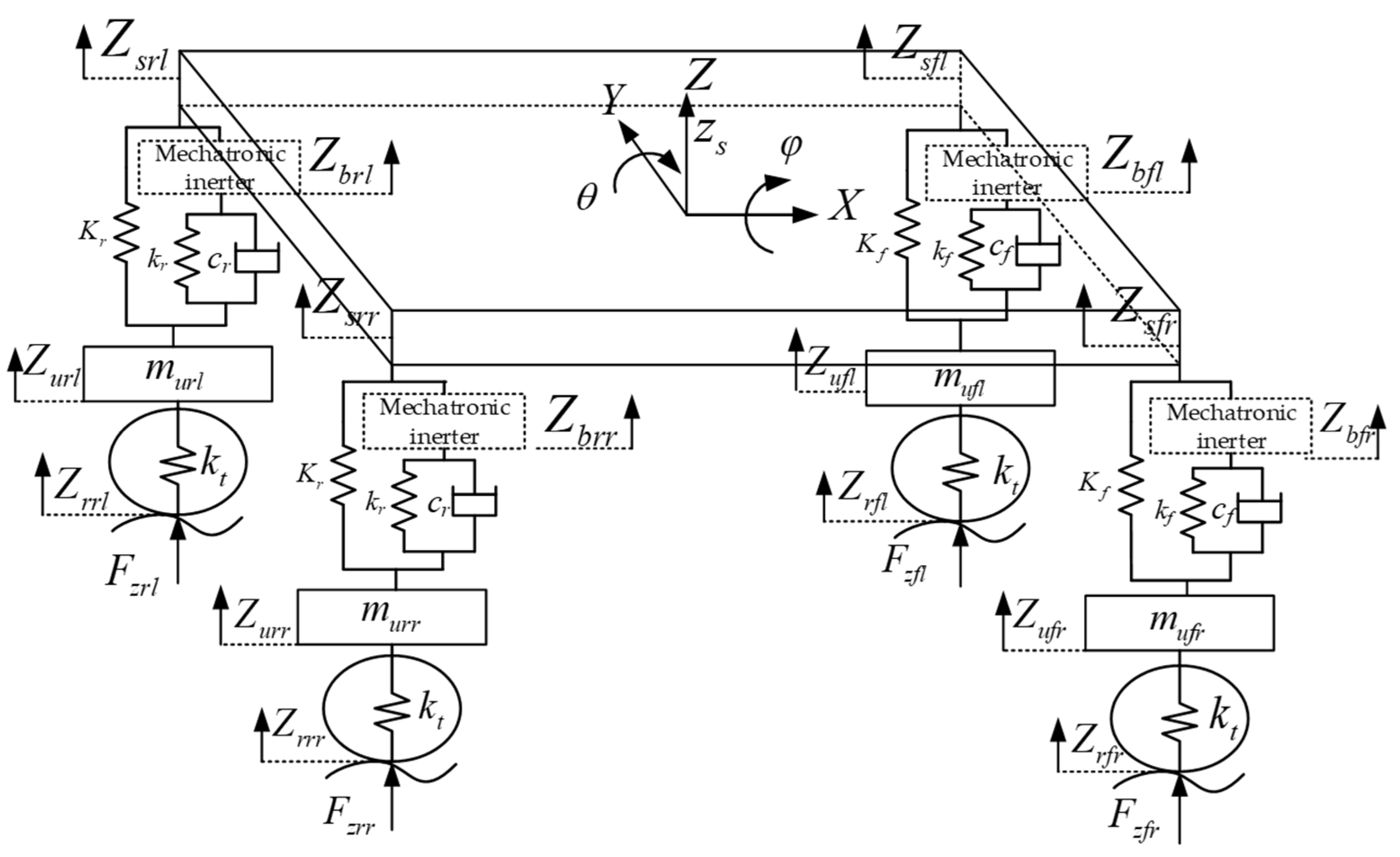
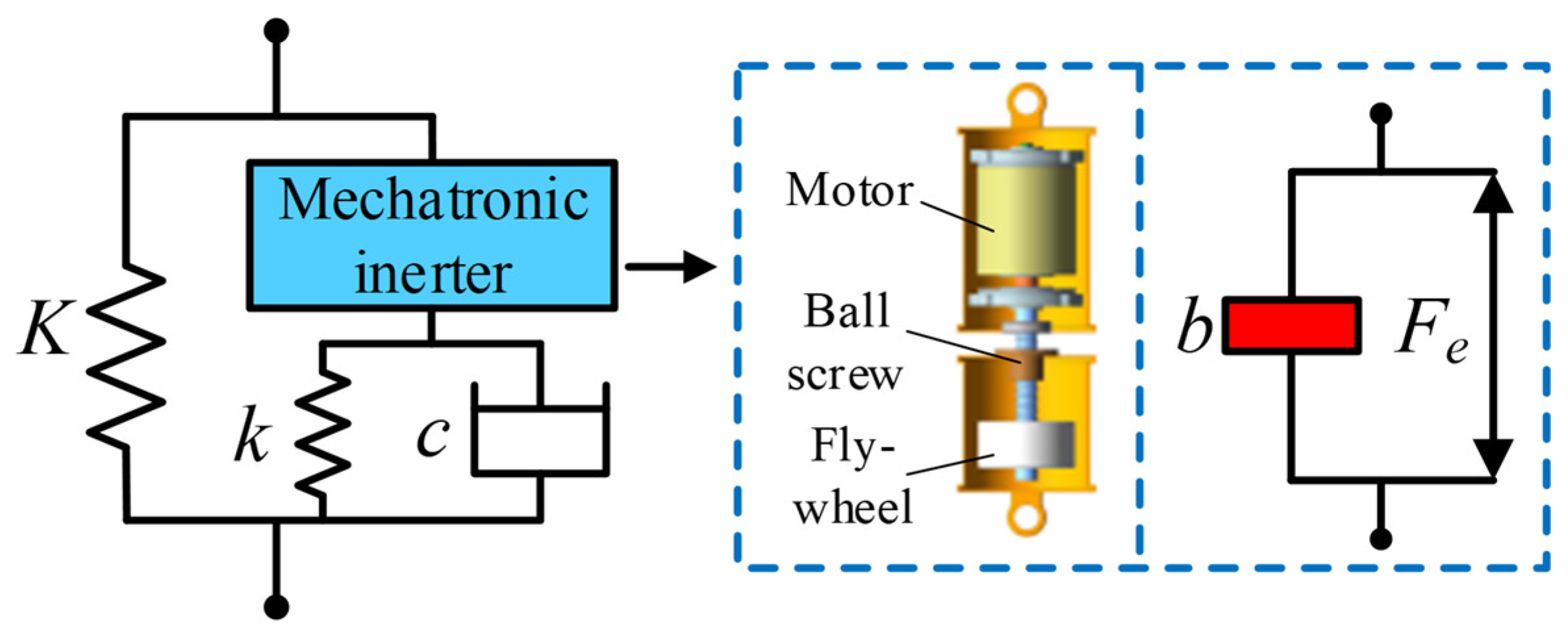
2. Vehicle Inertial Suspension Model

We consider the full-vehicle model depicted in Figure 1 to study the dynamic behavior of the vehicle suspension system. In this study, L4 is used as the inertial suspension structure [25].

As shown in Figure 2. The mechatronic inerter is connected to the spring and damper in series, and the load spring is connected to the mechatronic inerter, spring, and damper in parallel. The blue box shows the structure of the mechatronic inerter. The mechatronic inerter consisting of motor, ball screw and flywheel, When the mechatronic inerter is stimulated by vibration, the linear motion is converted into the rotating motion of the flywheel and motor through the ball screw, and the electromagnetic force generated by the motor is output in parallel with the inertial force.

The kinematic equation of the controlled model is

$$\left\{\begin{array}{l}{m}_s{\ddot{z}}_s=F_{fl}+F_{fr}+F_{rl}+F_{rr}\\ I_x\ddot{\phi }=m_t(\dot{v}+u\dot{\psi })h_2+m_{s}g{h}_1\mathit{sin}(\phi )+(F_{fl}-F_{fr}){\displaystyle \frac{w_f}{2}}+(F_{rl}-F_{rr}){\displaystyle \frac{w_r}{2}}\\ I_y\ddot{\theta }=m_t(\dot{u}-v\dot{\psi })h_3+m_{s}g{h}_1\mathit{sin}(\theta )+l_r(F_{rl}+F_{rr})-l_f(F_{fl}+F_{fr})\\ I_z\ddot{\psi }=l_f[(F_{yfl}+F_{yfr})\mathit{cos}(\delta )+(F_{xfl}+F_{xfr})\mathit{sin}(\delta )]-l_r(F_{yrl}+F_{yrr})\\ +{\displaystyle \frac{w_f}{2}}[(F_{xfr}-F_{xfl})\mathit{cos}(\delta )+(F_{yfl}-F_{yfr})\mathit{sin}(\delta )]+{\displaystyle \frac{w_r}{2}}(F_{xrr}-F_{xrl})\\ +(M_{zfl}+M_{zfr}+M_{zrl}+M_{zrr})\\ m_t(\dot{v}+u\dot{\psi })=(F_{xfl}+F_{xfr})\mathit{sin}(\delta )+(F_{yfl}+F_{yfr})\mathit{cos}(\delta )+F_{yrl}+F_{yrr}\\ m_t(\dot{u}-v\dot{\psi })=(F_{xfl}+F_{xfr})\mathit{cos}(\delta )-(F_{yfl}+F_{yfr})\mathit{sin}(\delta )+F_{xrl}+F_{xrr}\end{array}\right.$$

(1)

The vertical displacement equation for the four corners of the body is

$$\left\{\begin{array}{c}{Z}_{sfl}=z_s-l_f\theta +{\displaystyle \frac{w_f}{2}}\phi \\ Z_{sfr}=z_s-l_f\theta -{\displaystyle \frac{w_f}{2}}\phi \\ Z_{srl}=z_s+l_r\theta +{\displaystyle \frac{w_r}{2}}\phi \\ Z_{srr}=z_s+l_r\theta -{\displaystyle \frac{w_r}{2}}\phi \end{array}\right.$$

(2)

The equation of motion of the unsprung mass is

$$\left\{\begin{array}{c}{m}_{ufl}{\ddot{Z}}_{ufl}=k_t(Z_{rfl}-Z_{ufl})-F_{fl}\\ m_{ufr}{\ddot{Z}}_{ufr}=k_t(Z_{rfr}-Z_{ufr})-F_{fr}\\ m_{url}{\ddot{Z}}_{url}=k_t(Z_{rrl}-Z_{url})-F_{rl}\\ m_{urr}{\ddot{Z}}_{urr}=k_t(Z_{rrr}-Z_{urr})-F_{rr}\end{array}\right.$$

(3)

The suspension force equation is

$$\left\{\begin{array}{l}{F}_{fl}=K_f(Z_{ufl}-Z_{sfl})+F_{bfl}-{\displaystyle \frac{k_1}{2w_f}}(\phi -{\displaystyle \frac{Z_{ufl}-Z_{sfl}}{2w_f}})\\ F_{fr}=K_f(Z_{ufr}-Z_{sfr})+F_{bfr}-{\displaystyle \frac{k_1}{2w_f}}(\phi -{\displaystyle \frac{Z_{ufr}-Z_{sfr}}{2w_f}})\\ F_{rl}=K_r(Z_{url}-Z_{srl})+F_{brl}-{\displaystyle \frac{k_2}{2w_r}}(\phi -{\displaystyle \frac{Z_{url}-Z_{srl}}{2w_r}})\\ F_{rr}=K_r(Z_{urr}-Z_{srr})+F_{brr}-{\displaystyle \frac{k_2}{2w_r}}(\phi -{\displaystyle \frac{Z_{urr}-Z_{srr}}{2w_r}})\end{array}\right.$$

(4)

Among

$$\left\{\begin{array}{l}{F}_{bfl}=b_f({\ddot{Z}}_{bfl}-{\ddot{Z}}_{sfl})+F_{efl}=k_f(Z_{ufl}-Z_{bfl})+c_f({\dot{Z}}_{ufl}-{\dot{Z}}_{bfl})\\ F_{bfr}=b_f({\ddot{Z}}_{bfr}-{\ddot{Z}}_{sfr})+F_{efr}=k_f(Z_{ufr}-Z_{bfr})+c_f({\dot{Z}}_{ufr}-{\dot{Z}}_{bfr})\\ F_{brl}=b_r({\ddot{Z}}_{brl}-{\ddot{Z}}_{srl})+F_{erl}=k_r(Z_{url}-Z_{brl})+c_r({\dot{Z}}_{url}-{\dot{Z}}_{brl})\\ F_{brr}=b_r({\ddot{Z}}_{brr}-{\ddot{Z}}_{srr})+F_{err}=k_r(Z_{urr}-Z_{brr})+c_r({\dot{Z}}_{urr}-{\dot{Z}}_{brr})\end{array}\right.$$

(5)

The equation of the tire vertical load change is

$$\left\{\begin{array}{c}{F}_{zfl}=F_{fl}+m_{ufl}g+{\displaystyle \frac{m_{s}g{l}_r}{2(l_r+l_f)}}\\ F_{zfr}=F_{fr}+m_{ufr}g+{\displaystyle \frac{m_{s}g{l}_r}{2(l_r+l_f)}}\\ F_{zrl}=F_{rl}+m_{url}g+{\displaystyle \frac{m_{s}g{l}_f}{2(l_r+l_f)}}\\ F_{zrr}=F_{rr}+m_{urr}g+{\displaystyle \frac{m_{s}g{l}_f}{2(l_r+l_f)}}\end{array}\right.$$

(6)

where, $m_t$ represents the vehicle mass; $m_s$ indicates the sprung mass; $m_{ufl}$, $m_{ufr}$, $m_{url}$, and $m_{urr}$ represent the four wheel spring mass; $I_x$, $I_y$, and $I_z$ represent the moments of inertia of vehicle body roll, pitch, and yaw, respectively; $u$ represents the lateral speed of the vehicle; $v$ represents the lateral speed of the vehicle; $\psi$ represents the yaw angle; $\theta$ indicates the pitch angle; $\phi$ indicates the roll angle; $k_t$ denotes the radial stiffness of the tire; $z_s$ represents the vertical displacement of the body; $Z_{sfl}$, $Z_{sfr}$, $Z_{srl}$, and $Z_{srr}$ represent the vertical displacement of the sprung mass at the four corners of the body; $Z_{ufl}$, $Z_{ufr}$, $Z_{url}$, and $Z_{urr}$ represent the vertical displacement of unsprung mass; $Z_{rfl}$, $Z_{rfr}$, $Z_{rrl}$, and $Z_{rrr}$ represent road excitation; $k_1$ and $k_2$ represent the roll stiffness of front and rear suspension; $l_f$ and $l_r$ represent the distance from the center of mass to the front and rear wheels; $w_f$ and $w_r$ denote the front and rear wheel base; $h_1$ represents the distance between the body’s center of mass and the ground; $h_2$ indicates the distance from the roll center to the ground; $h_3$ represents the distance from the pitch center to the ground; $F_{fl}$, $F_{fr}$, $F_{rl}$, and $F_{rr}$ indicate the vertical load of suspension; $F_{zfl}$, $F_{zfr}$, $F_{zrl}$, and $F_{zrr}$ represent the vertical supporting force of the ground facing the tire; $F_{xfl}$, $F_{xfr}$, $F_{xrl}$, and $F_{xrr}$ indicate the longitudinal force of the tire; $F_{yfl}$, $F_{yfr}$, $F_{yrl}$, and $F_{yrr}$ indicate tire lateral force; $M_{zfl}$, $M_{zfr}$, $M_{zrl}$, and $M_{zrr}$ represent the tire righting torque; $b_f$ and $b_r$ are, respectively, the inertial coefficient of the front and rear wheel hydraulic and electric coupling inerter; $F_{bfl}$, $F_{bfr}$, $F_{brl}$, and $F_{brr}$ represent the output force of the left front wheel, right front wheel, left rear wheel, and right rear wheel suspension using the adjustable current of the inerter; $F_{efl}$, $F_{efr}$, $F_{erl}$, and $F_{err}$ represent the force of the mechatronic inerter in the left front wheel, right front wheel, left rear wheel, and right rear wheel suspension, respectively; $c_f$ and $c_r$ are the damping coefficient of the front and rear wheel suspension, respectively; $k_f$ and $k_r$ are the secondary spring stiffness of the front and rear wheel suspension, respectively; and $Z_{bfl}$, $Z_{bfr}$, $Z_{brl}$, and $Z_{brr}$ represent the vertical displacement of the mechatronic inerter of the left front wheel, right front wheel, left rear wheel, and right rear wheel suspension, respectively.

Aiming at the control of ride comfort, this paper takes the body vibration acceleration, pitch angle acceleration, and roll angle acceleration as the control targets, while taking into account the vertical, pitch, and roll movements of the vehicle. Therefore, the dynamics equations of vertical, pitch, and roll movements in the vehicle model are rewritten as follows:

$$\left\{\begin{array}{l}{\ddot{z}}_s=f_{z_s}(z_s,t)+g_{z_s}(z_s,t)u_{z_s}\\ \ddot{\theta }=f_{\theta }(\theta ,t)+g_{\theta }(\theta ,t)u_{\theta }\\ \ddot{\phi }=f_{\phi }(\phi ,t)+g_{\phi }(\phi ,t)u_{\phi }\end{array}\right.$$

(7)

From the above formula, $f_{z_s}(z_s,t)$, $f_{\theta }(\theta ,t)$, and $f_{\phi }(\phi ,t)$ can be found in Appendix A points 1, 2, and 3.

$$\left\{\begin{array}{l}{g}_{z_s}(z_s,t)=1/m_s\\ g_{\theta }(\theta ,t)=1/I_y\\ g_{\phi }(\phi ,t)=1/I_x\end{array}\right.$$

(8)

$$\left\{\begin{array}{l}{u}_{z_s}=F_{efl}+F_{efr}+F_{erl}+F_{err}\\ u_{\theta }=-l_f(F_{efl}+F_{efr})+l_r(F_{erl}+F_{err})\\ u_{\phi }={\displaystyle \frac{w_f}{2}}(F_{efl}-F_{efr})+{\displaystyle \frac{w_r}{2}}(F_{erl}-F_{err})\end{array}\right.$$

(9)

The parameters of the whole car model are from a mature passenger car, and the detailed parameters are shown in

Table 1. Vehicle model parameters.

Parameter	Value
Vehicle mass mt/(kg)	1659
Sprung mass ms/(kg)	1410
Front wheel unsprung mass mufl, mufr/(kg)	26.5
Rear wheel unsprung mass murl, murr/(kg)	24.4
Front wheel base wf/(m)	1.574
Rear wheel base wr/(m)	1.593
Distance from front axle to center of mass lf/(m)	1.278
Distance from rear axis to center of mass lr/(m)	1.430
Height of center of mass h1/(m)	0.50
Roll height h2/(m)	0.40
Distance from center of roll to center of mass h3/(m)	0.25
Body roll moment of inertia Ix/(kg·m2)	925
Body pitch moment of inertia Iy/(kg·m2)	2577
Body yaw moment of inertia Iz/(kg·m2)	2603
Wheel inertia Iw/(kg·m2)	0.99
Wheel radius Rw/(m)	0.345
Front suspension roll stiffness k1/(N·m·rad−1)	47,298
Rear suspension roll stiffness k2/(N·m·rad−1)	37,311
Tire equivalent spring stiffness kt/(N/m)	192,000
Front suspension spring stiffness of the original model Kf/(N·m−1)	25,000
Rear suspension spring stiffness of the original model Kr/(N·m−1)	22,000
Front suspension spring stiffness kf/(N·m−1)	9325
Rear suspension spring stiffness kr/(N·m−1)	7897
Front suspension damping coefficient cf/(N·s·m−1)	1579
Rear suspension damping coefficient cr/(N·s·m−1)	1407
Front suspension inertial coefficient bf/(kg)	330
Rear suspension inertial coefficient br/(kg)	265

.

The single wheel pavement input model with white noise as the excitation source of random pavement input is mathematically expressed as [26]:

$${\dot{Z}}_r\left(t\right)=-2\pi f_0{Z}_r\left(t\right)+2\pi \sqrt{G_{0}u}w\left(t\right)$$

(10)

where G₀ is the road roughness coefficient, set to 256 × 10⁻⁶ m⁻³. u is the speed and w(t) is the integral white noise. Assuming the vehicle is traveling at a speed of 20 m/s, the difference in excitation between the front and rear wheels is a delay determined by the speed and the length of the front to rear wheels. The unevenness displacement of the left front wheel and the right front wheel is shown in Figure 3.

3. Optimization of Vehicle Inertial Suspension Parameters

In this paper, the NSGA-II algorithm is used to optimize inertial suspension parameters, mainly considering vehicle ride comfort. The algorithm flowchart is shown in Figure 4. The optimal individual coefficient is set at 0.3, the population size amounts to 200, the number of iterations is 100, the stopping criterion is reached after 200 generations, and the deviation of the fitness function is 10⁻¹⁰.

To evaluate vehicle ride comfort, the RMS values of body vertical acceleration, lateral camber acceleration, and pitch angle acceleration were selected as the optimization objectives. In the optimization process, in order to reflect the effect of the inerter, we keep the stiffness of the support spring unchanged, and other parameters to be optimized are the following:

$$X=[k_f,k_r,c_f,c_r,b_f,b_r]$$

(11)

The objective function $J_1$, $J_2$, $J_3$ is obtained:

$$\left\{\begin{array}{c}\mathit{min}{J}_1={\displaystyle \frac{BA\left(X\right)}{B{A}_{pass}}}\\ \mathit{min}{J}_2={\displaystyle \frac{RA\left(X\right)}{R{A}_{pass}}}\\ \mathit{min}{J}_3={\displaystyle \frac{PA\left(X\right)}{P{A}_{pass}}}\end{array}\right.$$

(12)

In the above formula, $J_1$, $J_2$, and $J_3$, respectively, represent the objective function of body acceleration, pitch angle acceleration, and roll angle acceleration; $BA\left(X\right)$, $PA\left(X\right)$, and $RA\left(X\right)$, respectively, represent the RMS values of body, pitch angle, and roll angle acceleration of the inertial suspension to be optimized; $B{A}_{pass}$, $P{A}_{pass}$, and $R{A}_{pass}$, respectively, represent the RMS values of body, pitch angle, and roll angle acceleration of passive suspension.

Firstly, the performance indicators for evaluating vehicle ride comfort in vertical, pitch, and roll directions should not be worse than those of passive suspension. Then, in the design of suspension parameters, considering that the working space between the wheel and the body is limited to a certain range to ensure better grip when the wheel is in contact with the road, the working space of the designed inertial suspension and the dynamic load of the tire are smaller than those of the passive suspension. Therefore, the optimization conditions are as follows:

$$st\left\{\begin{array}{l}BA\left(X\right)<B{A}_{pass}\\ RA\left(X\right)<R{A}_{pass}\\ PA\left(X\right)<P{A}_{pass}\\ DTL\left(X\right)\le DT{L}_{pass}\\ SWS\left(X\right)\le SW{S}_{psss}\\ UB<X<LB\end{array}\right.$$

(13)

In the above formula: $DTL\left(X\right)$ is the RMS value of the dynamic tire load of the left front wheel suspension; $SWS\left(X\right)$ represents the RMS value of the suspension working space of the left front wheel; $DT{L}_{pass}$ represents the RMS value of the dynamic tire load of the left front wheel passive suspension; $SW{S}_{psss}$ represents the RMS value of suspension working space of the left front wheel passive suspension; $UB$ represents the lower limit of the optimization target parameter, the values for [10,000, 10,000, 500, 500, 1, 1]; and $LB$ represents the upper limit of the optimization target parameter, the values for [40,000, 40,000, 4000, 4000, 1000, 1000]. When the vehicle is driving in a straight line at a speed of 20 m/s on a Class C random road surface, the performance indicators of the passive suspension are shown in

Table 2. Performance indicators of passive suspension.

Performance Indicators	RMS Value
Body acceleration/(m·s−2)	1.3644
Roll angle acceleration/(rad·s−2)	0.8326
Pitch angle acceleration/(rad·s−2)	0.7094
Left front wheel suspension working space/(m)	0.0225
Left front dynamic tire load/(kN)	1.1633
Right front wheel suspension working space/(m)	0.0151
Right front wheel dynamic tire load/(kN)	0.8796
Left rear wheel suspension working space/(m)	0.0180
Left rear wheel dynamic tire load/(kN)	1.0851
Right rear wheel suspension working space/(m)	0.0157
Right rear wheel dynamic tire load/(kN)	0.8787

.

After optimization by the NSGA-II algorithm, the component parameters of four kinds of inertial suspension structures are obtained. The results of parameter optimization are shown in

Table 3. Parameter optimization results.

Optimization Parameter	Value
Front suspension spring stiffness/(N·m−1)	9325
Rear suspension spring stiffness/(N·m−1)	7897
Front suspension damping coefficient/(N·s·m−1)	1579
Rear suspension damping coefficient/(N·s·m−1)	1407
Front suspension inertial coefficient/(kg)	330
Rear suspension inertial coefficient/(kg)	265

.

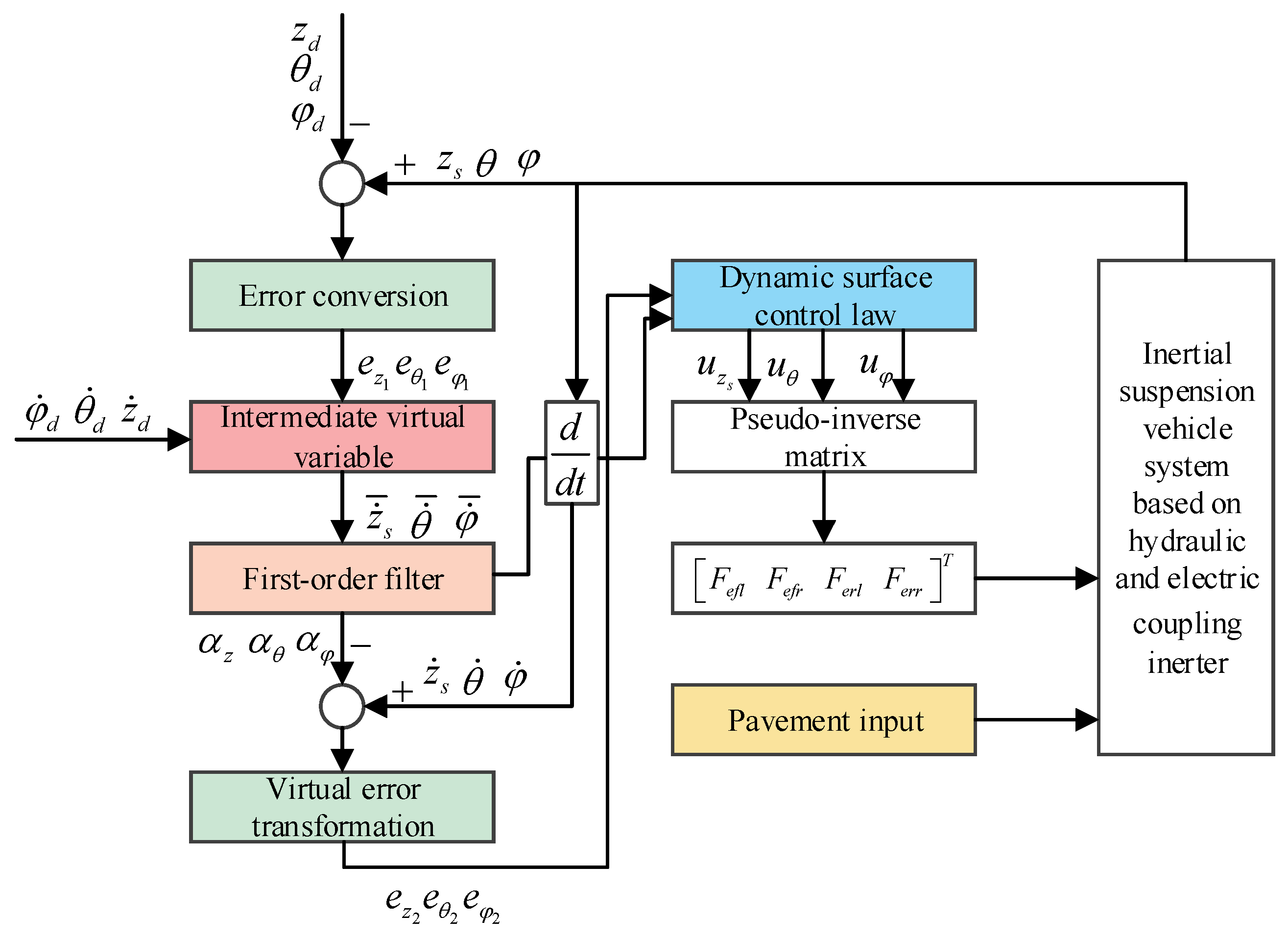
4. Design of Coordination Controller Based on Dynamic Surface Control Theory

4.1. Controller Design Procedure

In this paper, the controller actually needs the ideal displacement $z_d$, the ideal pitch angle ${\theta }_d$, and the ideal roll angle ${\phi }_d$ of the body.

First, the ideal displacement of the vertical motion of the body is defined as $z_d$, so the position error is defined as

$$e_{z_1}=z_s-z_d$$

(14)

To ensure that $u_{z_s}$ causes $e_{z_1}$ to converge to 0, the derivative of $e_{z_1}$ yields

$${\dot{e}}_{z_1}={\dot{z}}_s-{\dot{z}}_d$$

(15)

We design the Lyapunov function

$$V_1={\displaystyle \frac{1}{2}}{e}_{z_1}^2$$

(16)

Then

$${\dot{V}}_1={\dot{e}}_{z_1}{e}_{z_1}=({\dot{z}}_s-{\dot{z}}_d)e_{z_1}$$

(17)

Assuming an intermediate dummy variable ${\alpha }_z$, to make ${\dot{V}}_1$ less than or equal to 0, we define $e_{z_2}={\dot{z}}_s-{\alpha }_z$, then

$${\dot{V}}_1=(e_{z_2}+{\alpha }_z-{\dot{z}}_d)e_{z_1}$$

(18)

In the Backstepping design, the intermediate virtual variable is designed as ${\alpha }_z=-c_{z_1}{e}_{z_1}+{\dot{z}}_d$, where $c_{z_1}$ is a positive real number, which can satisfy the stability of Lyapunov function. However, differentiation explosion will occur when differentiating the intermediate virtual variable, which increases the workload of the computer and the simulation time. Therefore, dynamic surface control adopts a low-pass filter to avoid this defect.

The control law of the intermediate virtual variable in the Backstepping design is defined as ${\bar{\dot{z}}}_s=-c_{z_1}{e}_{z_1}+{\dot{z}}_d$, ${\alpha }_z$ is output through the low-pass filter ${\displaystyle \frac{1}{\tau s+1}}$, and intermediate virtual variable ${\alpha }_z$ satisfies

$$\left\{\begin{array}{l}\tau {\dot{\alpha }}_z+{\alpha }_z={\bar{\dot{z}}}_s\\ {\alpha }_z(0)={\bar{\dot{z}}}_s(0)\end{array}\right.$$

(19)

Equation (6) can obtain ${\dot{\alpha }}_z={\displaystyle \frac{{\bar{\dot{z}}}_s-{\alpha }_z}{\tau }}$, and its filtering error is $y_2={\alpha }_z-{\bar{\dot{z}}}_s$.

The design of the Lyapunov function satisfying position, intermediate dummy variable, and filtering error is as follows:

$$V_2={\displaystyle \frac{1}{2}}{e}_{z_1}^2+{\displaystyle \frac{1}{2}}{e}_{z_2}^2+{\displaystyle \frac{1}{2}}{y}_2^2$$

(20)

Taking the derivative of this gives us ${\dot{V}}_2$:

$${\dot{V}}_2=e_{z_1}{\dot{e}}_{z_1}+e_{z_2}{\dot{e}}_{z_2}+y_2{\dot{y}}_2$$

(21)

From ${\dot{e}}_{z_2}={\ddot{z}}_s-{\dot{\alpha }}_z=f_{z_s}(z_s,t)+g_{z_s}(z_s,t)u_{z_s}-{\displaystyle \frac{{\bar{\dot{z}}}_s-{\alpha }_z}{\tau }}$, ${\dot{y}}_2={\dot{\alpha }}_z-{\dot{\bar{\dot{z}}}}_s={\displaystyle \frac{-y_2}{\tau }}+c_{z_1}{\dot{e}}_{z_1}-{\ddot{z}}_d$, The converted ${\dot{V}}_2$ are presented in Appendix A point 4.

The dynamic surface control law is set as

$$u_{z_s}={\displaystyle \frac{1}{g_{z_s}(z_s,t)}}(-f_{z_s}(z_s,t)+{\dot{\alpha }}_z-c_{z_2}{e}_{z_2})$$

(22)

where $c_{z_2}$ is a positive real number, and the same can be obtained:

$$u_{\theta }={\displaystyle \frac{1}{g_{\theta }(\theta ,t)}}(-f_{\theta }(\theta ,t)+{\dot{\alpha }}_{\theta }-c_{{\theta }_2}{e}_{{\theta }_2})$$

(23)

$$u_{\phi }={\displaystyle \frac{1}{g_{\phi }(\phi ,t)}}(-f_{\phi }(\phi ,t)+{\dot{\alpha }}_{\phi }-c_{{\phi }_2}{e}_{{\phi }_2})$$

(24)

According to the control force and control moment obtained by vertical, roll, and pitch motion, the force of mechatronic inerter in four suspensions can be obtained, which can be sorted as

$$A_{f}X=b_f$$

(25)

$$b_f=\left[\begin{array}{c}{u}_{z_s}\\ u_{\theta }\\ u_{\phi }\end{array}\right],A_f=\left[\begin{array}{cccc}1& 1& 1& 1\\ -l_f& -l_f& l_r& l_r\\ {\displaystyle \frac{w_f}{2}}& -{\displaystyle \frac{w_f}{2}}& {\displaystyle \frac{w_r}{2}}& -{\displaystyle \frac{w_r}{2}}\end{array}\right],X=\left[\begin{array}{c}{F}_{efl}\\ F_{efr}\\ F_{erl}\\ F_{err}\end{array}\right]$$

(26)

When there is a solution to Equation (25), it is equivalent to $rank\left(A_f\right)=rank(A_f,b_f)$, that is, the number of linearly independent columns that need to satisfy the coefficient matrix is the same as the number of linearly independent columns of the augmented matrix. From Formula (26), it can be calculated that

$$rank\left(A_f\right)=3,\hspace{1em}rank(A_f,b_f)=3$$

(27)

Since $A_f$ is 3 × 4 dimensional matrix, that is, $A_f$ is not a square matrix, it is impossible to solve the linear equations in the form of computational matrices by finding the inverse matrix of $A_f$. Therefore, this paper constructs a generalized inverse matrix solution for $A_f$, then the pseudo-inverse matrix $C^{*}$ of $A_f$ is $C^{*}=(A_f^T{A}_f{)}^{-1}{A}_f^T$, and $C^{*}{A}_f=I$ can be obtained, $I$ is the identity matrix, and its expression is $C^{*}=pinv\left(A_f\right)$. Thus, the force of mechatronic inerter can be obtained:

$$\left[\begin{array}{c}{F}_{efl}\\ F_{efr}\\ F_{erl}\\ F_{err}\end{array}\right]=C^{*}\left[\begin{array}{c}{u}_{z_s}\\ u_{\theta }\\ u_{\phi }\end{array}\right]$$

(28)

Therefore, the schematic diagram of the dynamic surface control system designed in this paper is shown in Figure 5. The road input offers external excitation. Vertical displacement and pitch and roll angle are derived from the dynamic inertial suspension system based on the hydraulic and electric coupling inerter, and the error equation is acquired with the predefined ideal vertical displacement and pitch and roll angle. Through intermediate virtual variable and first-order filter, the dynamic surface control law of vertical, pitch, and roll motion is obtained, and the pseudo-inverse matrix is constructed to address the issue. The electromagnetic force of the four suspensions can be obtained.

4.2. Stability Proof

Then, the stability of the designed dynamic surface control law is analyzed by Lyapunov stability criterion.

If $V_2\left(0\right)\le p$, $p>0$ is taken, then all signals in the closed loop system are in a bounded closed set, that is, in a compact set.

Proof. 

If $V_2=p$, $V_2={\displaystyle \frac{1}{2}}{e}_{z_1}^2+{\displaystyle \frac{1}{2}}{e}_{z_2}^2+{\displaystyle \frac{1}{2}}{y}_2^2=p$, and since $A$ is a function of $e_{z_1},e_{z_2},y_2,{\ddot{z}}_d$, then $A$ is bounded, denoted $B$, then ${\displaystyle \frac{A^2}{B^2}}-1\le 0$.

$$\begin{array}{l}{\dot{V}}_2=e_{z_1}\left(e_{z_2}+y_2\right)-c_{z_1}{e}_{z_1}^2-c_{z_2}{e}_{z_2}^2+y_2\left({\displaystyle \frac{-y_2}{\tau }}+A\right)\\ \le \left|e_{z_1}\right|\left|e_{z_2}\right|+\left|e_{z_1}\right|\left|y_2\right|-c_{z_1}{e}_{z_1}^2-c_{z_2}{e}_{z_2}^2-{\displaystyle \frac{1}{\tau }}{y}_2^2+\left|A\right|\left|y_2\right|\\ \le {\displaystyle \frac{1}{2}}\left(e_{z_1}^2+e_{z_2}^2\right)+{\displaystyle \frac{1}{2}}\left(e_{z_1}^2+y_2^2\right)-c_{z_1}{e}_{z_1}^2-c_{z_2}{e}_{z_2}^2-{\displaystyle \frac{1}{\tau }}{y}_2^2+{\displaystyle \frac{1}{2}}{y}_2^2{A}^2+{\displaystyle \frac{1}{2}}\\ =\left(1-c_{z_1}\right)e_{z_1}^2+({\displaystyle \frac{1}{2}}-c_{z_2})e_{z_2}^2+({\displaystyle \frac{1}{2}}{A}^2+{\displaystyle \frac{1}{2}}-{\displaystyle \frac{1}{\tau }})y_2^2+{\displaystyle \frac{1}{2}}\end{array}$$

(29)

When $c_{z_1}\ge 1+r,c_{z_2}\ge {\displaystyle \frac{1}{2}}+r,{\displaystyle \frac{1}{\tau }}\ge {\displaystyle \frac{1}{2}}B+{\displaystyle \frac{1}{2}}+r,r>0$, then

$$\begin{array}{l}{\dot{V}}_2\le -r{e}_{z_1}^2-r{e}_{z_2}^2+\left({\displaystyle \frac{1}{2}}{A}^2-{\displaystyle \frac{B^2}{2}}-r\right)y_2^2+{\displaystyle \frac{1}{2}}\\ =-2r{V}_2+\left({\displaystyle \frac{B^2}{2B^2}}{A}^2-{\displaystyle \frac{B^2}{2}}\right)y_2^2+{\displaystyle \frac{1}{2}}=-2r{V}_2+\left({\displaystyle \frac{A^2}{B^2}}-1\right){\displaystyle \frac{B^2{y}_2^2}{2}}+{\displaystyle \frac{1}{2}}\\ \le -2r{V}_2+{\displaystyle \frac{1}{2}}\end{array}$$

(30)

$V_2=p$ is known from the condition, so Equation (30) can be changed to ${\dot{V}}_2\le -2rp+{\displaystyle \frac{1}{2}}$.

Therefore, in order to ensure that ${\dot{V}}_2$ is negative definite, that is, to ensure the stability of the control system, $-2rp+{\displaystyle \frac{1}{2}}\le 0$ is $r\ge {\displaystyle \frac{p}{4}}$.

That is, it has been proven that when $r\ge {\displaystyle \frac{p}{4}}$, all the information of the closed-loop control system is in the compact set, that is, if $V_2\left(0\right)\le p$, then ${\dot{V}}_2\le 0$, and thus $V_2\left(t\right)\le p$. □

Lemma 1.

For any$V:[0,\infty )\in R$, the solution of the inequality equation  $\dot{V}\le -\alpha V+f,\forall t\ge t_0\ge 0$ is 

$$V(t)\le e^{-\alpha (t-t_0)}V(t_0)+{\int }_{t_0}^t{e}^{-\alpha (t-\tau )}f\left(\tau \right)d\tau ,\forall t\ge t_0\ge 0$$

(31)

where  $\alpha$ is a real number.

According to the conclusion of Lemma 1, Formula (32): ${\dot{V}}_2\le -2r{V}_2+{\displaystyle \frac{1}{2}}$ is solved and its convergence is analyzed, then Formula (32) can be rewritten as:

$$\begin{array}{l}{V}_2\left(t\right)\le e^{-2r\left(t-t_0\right)}{V}_2\left(t_0\right)+0.5e^{-2rt}{\int }_{t_0}^t{e}^{{\eta }_1\tau }d\tau \\ =e^{-2r\left(t-t_0\right)}{V}_2\left(t_0\right)+{\displaystyle \frac{0.5e^{-2rt}}{2r}}\left(e^{2rt}-e^{2r{t}_0}\right)\\ =e^{-2r(t-t_0)}{V}_2\left(t_0\right)+{\displaystyle \frac{1}{4r}}(1-e^{-2r(t-t_0)})\end{array}$$

(32)

Obtain

$$\underset{t\to \infty }{lim}{V}_2(t)\le {\displaystyle \frac{1}{4r}}$$

(33)

Note $V_2\left(t\right)$ converges progressively and is determined by $r$.

Then, when ${\displaystyle \frac{1}{\tau }}\ge {\displaystyle \frac{1}{2}}B+{\displaystyle \frac{1}{2}}+r$, take $\tau \to 0$, then $r\to \infty$. That is what $\tau$ is based on.

The unknown parameter can be set according to the stability condition. The value of $\tau$ is 0.01. Since $r\ge {\displaystyle \frac{p}{4}}$ and $p$ are related to the initial value, set to 2, then $r$ can be 1. Because of $c_{z_1}\ge 1+r,c_{z_2}\ge {\displaystyle \frac{1}{2}}+r$, then $c_{z_1},c_{z_2}$ take 16 and 2.5, respectively. Similarly,$c_{{\theta }_1},c_{{\theta }_2}$ and $c_{{\phi }_1},c_{{\phi }_2}$ are both 2 and 2.5. The linear driving has a greater influence on the acceleration of the vehicle body, so the gain value of $c_{z_1},c_{z_2}$ is larger.

5. Performance Analysis of Inertial Suspension Based on Dynamic Surface Control

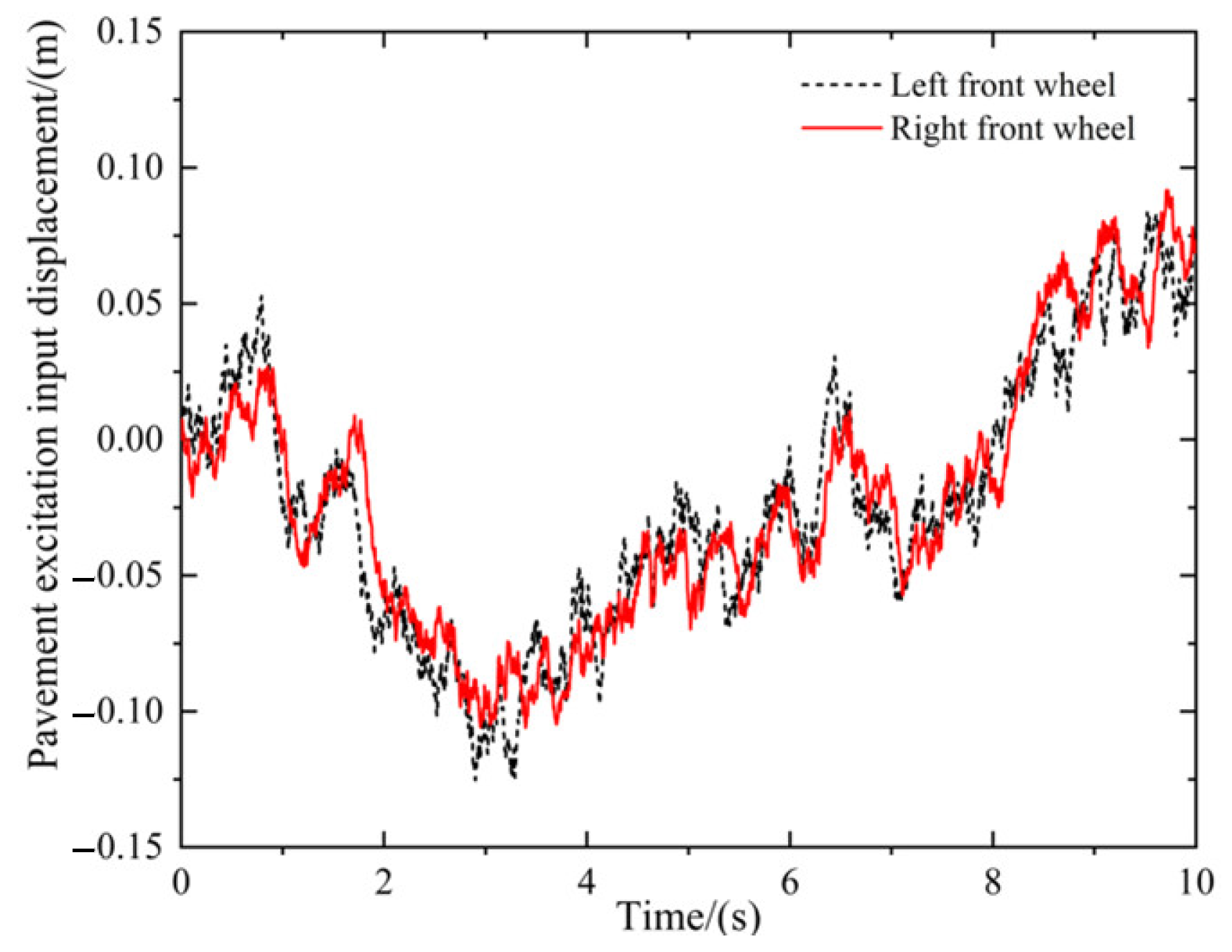
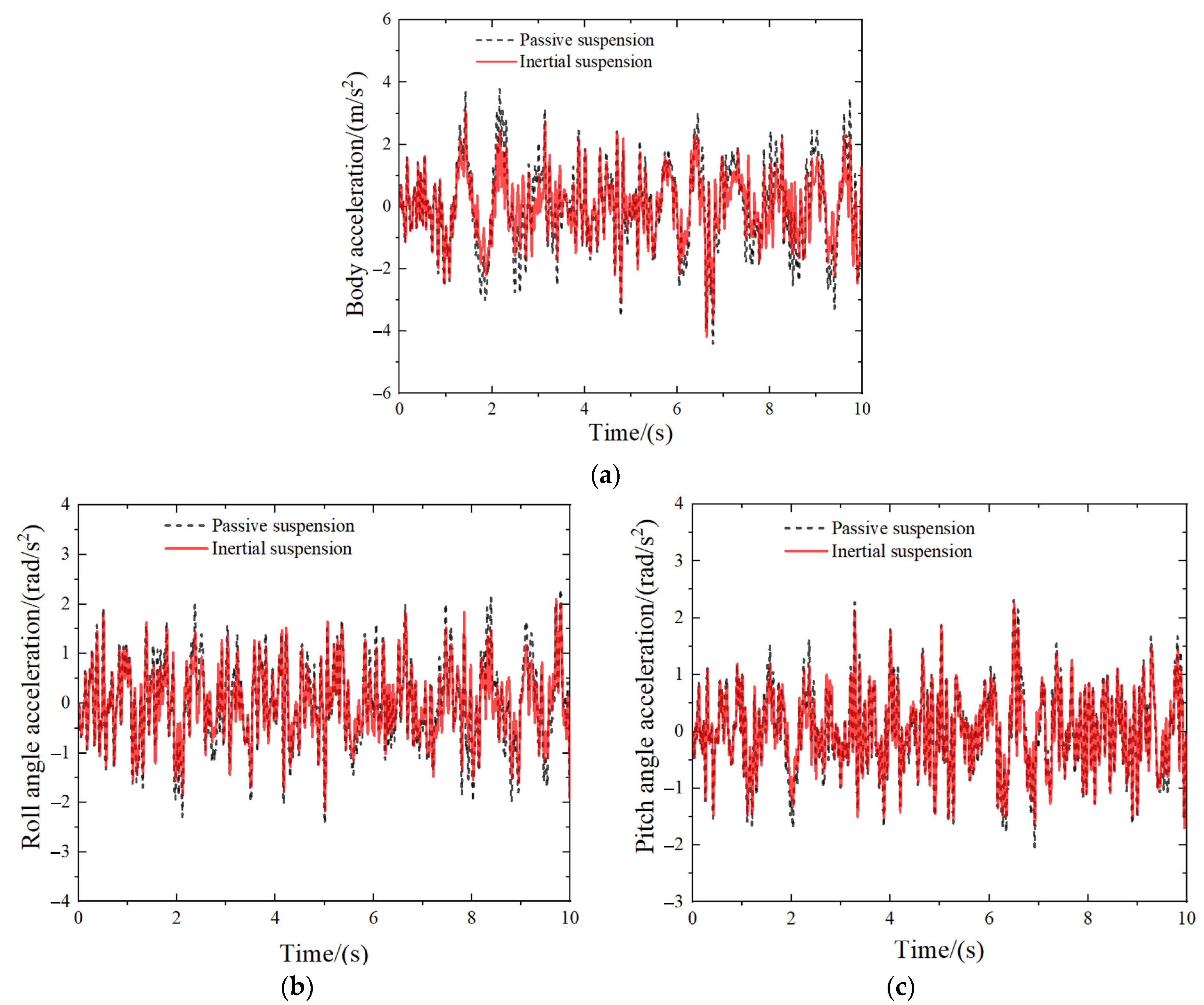
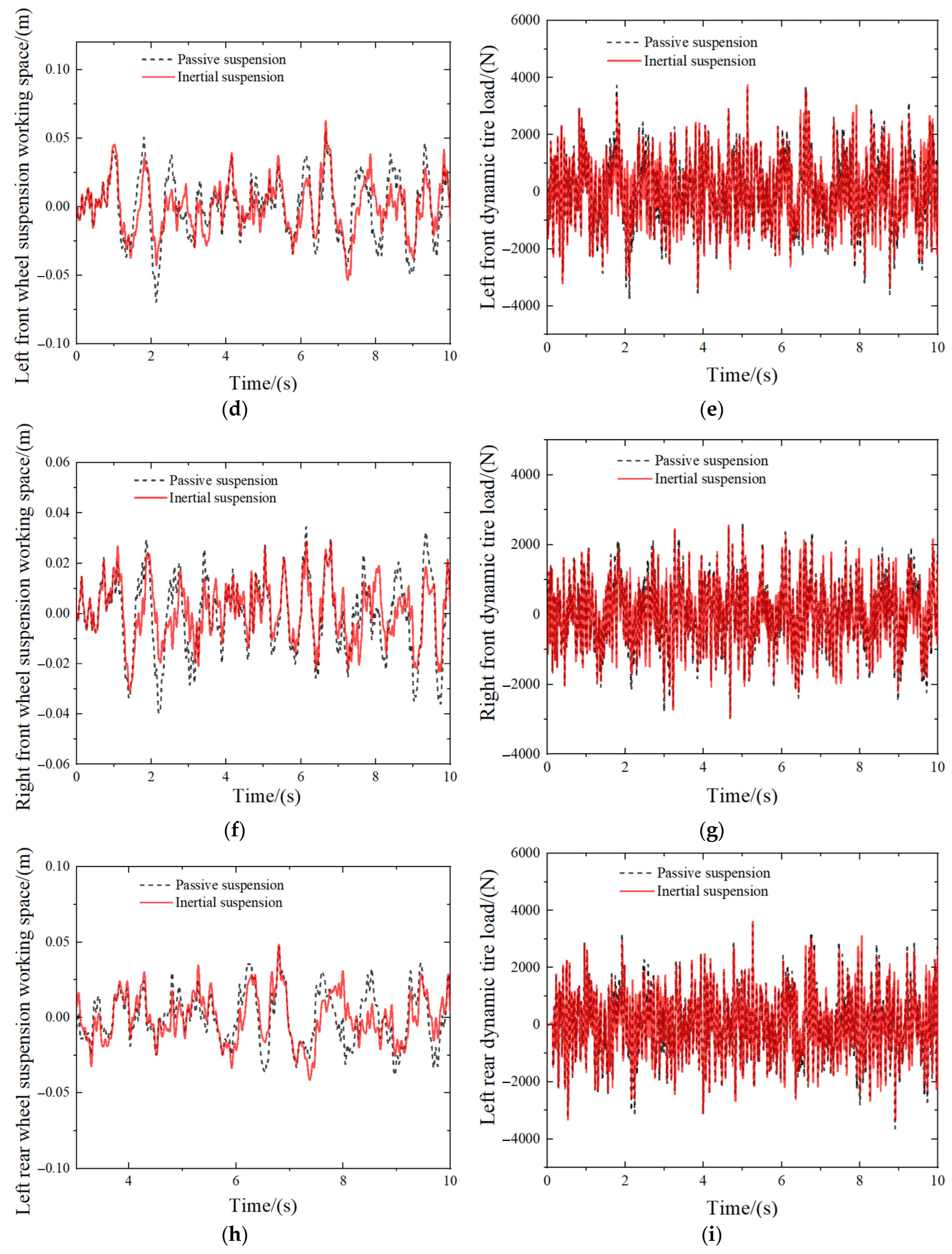
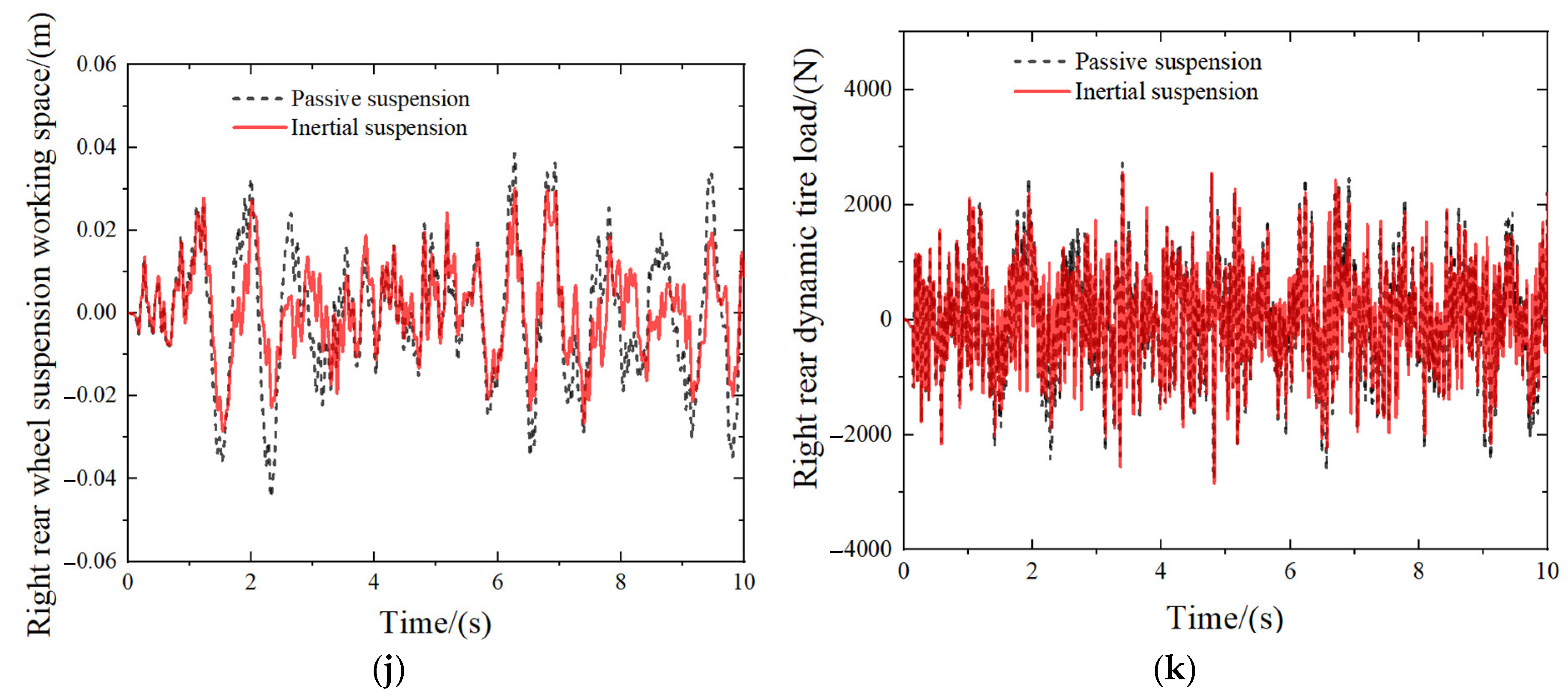
5.1. Time Domain Performance Analysis

In order to analyze the mechanical properties of suspension, a speed of 20 m/s was selected for simulation, and the road input was set as C-class random road input. Figure 6 shows the performance response comparison of passive suspension and Inertial suspension, while

Table 4. Performance comparison table of inertial suspension.

The RMS Values	Passive Suspension	Inertial Suspension	Performance Improvement
Body acceleration/(m·s−2)	1.3644	1.0406	23.73%
Roll angle acceleration/(rad·s−2)	0.8326	0.7054	15.28%
Pitch angle acceleration/(rad·s−2)	0.7094	0.6495	8.44%
Left front wheel suspension working space/(m)	0.0225	0.0191	15.27%
Left front dynamic tire load/(kN)	1.1633	1.0999	5.45%
Right front wheel suspension working space/(m)	0.0151	0.0116	23.21%
Right front dynamic tire load/(kN)	0.8796	0.8272	5.95%
Left rear wheel suspension working space/(m)	0.0180	0.0158	12.05%
Left rear dynamic tire load/(kN)	1.0851	1.0469	3.52%
Right rear wheel suspension working space/(m)	0.0157	0.0112	28.57%
Right rear dynamic tire load/(kN)	0.8787	0.8166	7.06%

shows the RMS values comparison of performance indicators of passive suspension and inertial suspension.

As can be observed from the time domain comparison presented in Figure 6, the acceleration of the vehicle body and the acceleration of the side angle are conspicuously suppressed throughout the entire time domain. The suspension working space of the four-wheel is significantly smaller than that of the passive suspension. The acceleration of the pitch angle and the dynamic tire load of the four-wheel are marginally less than those of the passive suspension. As can be seen from Table 4, the performance of the inertial suspension based on dynamic surface control is significantly better than that of the passive suspension. Compared with the passive suspension, the RMS value of the body acceleration of the inertial suspension decreases by 23.73%. Compared with that of the passive suspension, the RMS of the performance indicators of the roll angle acceleration of the inertial suspension decreased by 15.28%. For the RMS of pitch angle acceleration, the performance of inertial suspension improved by 8.44%. In addition, the RMS of dynamic tire load of the controllable inertial suspension also decreased to a certain extent. In terms of the RMS of the suspension working space, the performance of the inertial suspension with the RMS of the suspension working space of the right front wheel suspension and the right rear wheel suspension was significantly improved by 23.21%, and the improvement effect of the left front wheel suspension and the left rear wheel suspension was better than that of the passive suspension. A comprehensive analysis of Figure 6 shows that the inertial suspension based on dynamic surface control achieves the goal of improving ride comfort, and its performance indicators are superior to that of the passive suspension.

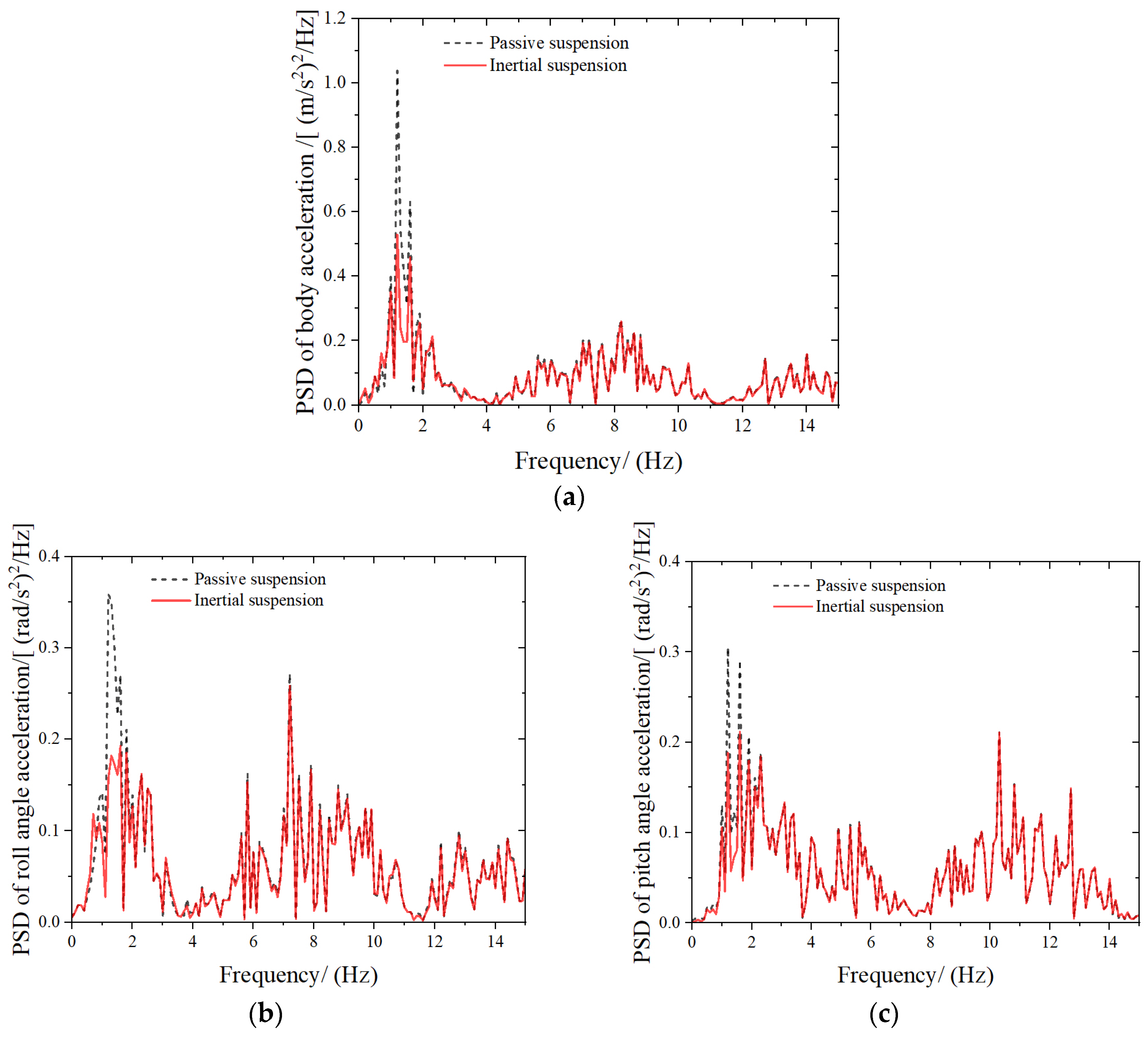
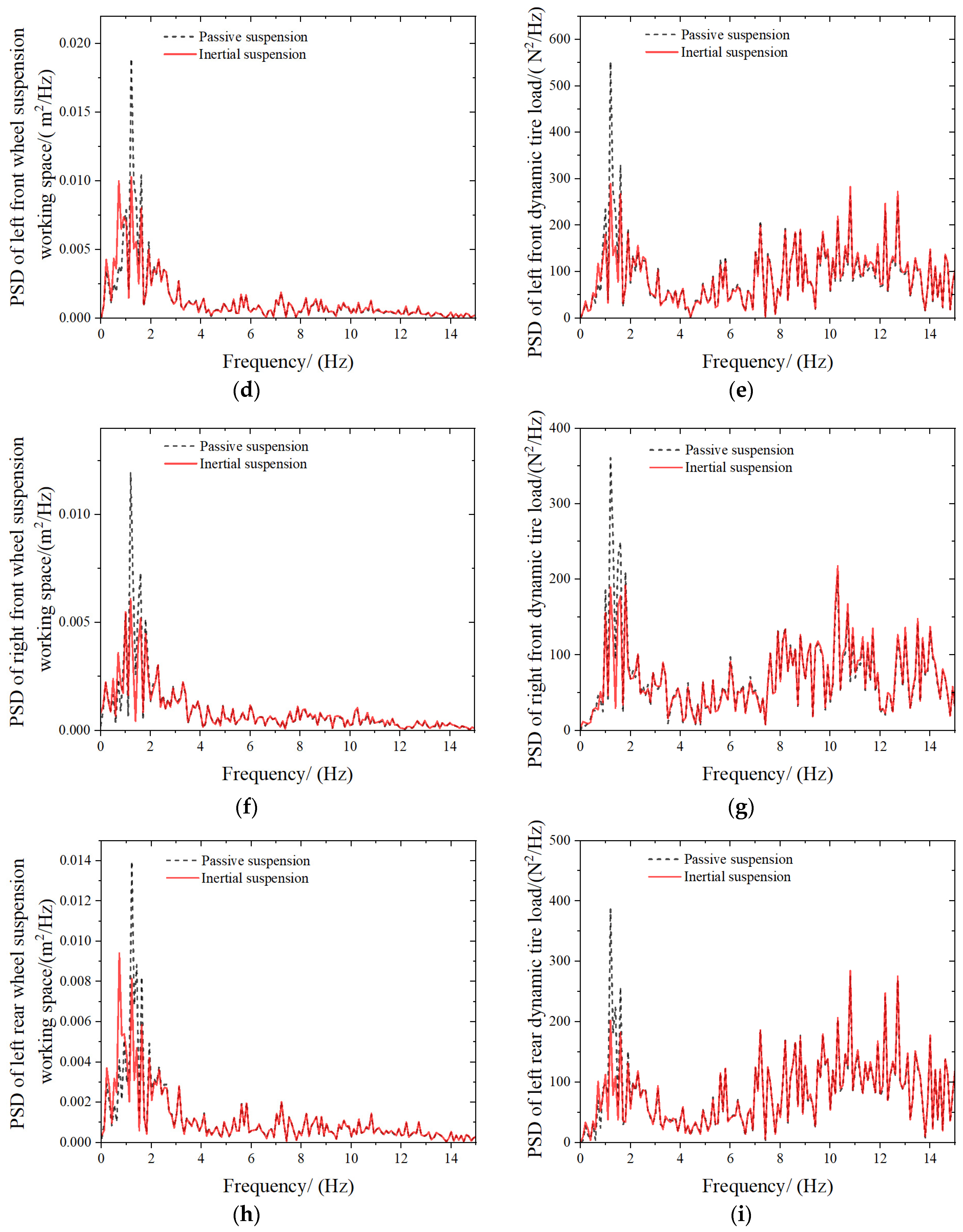
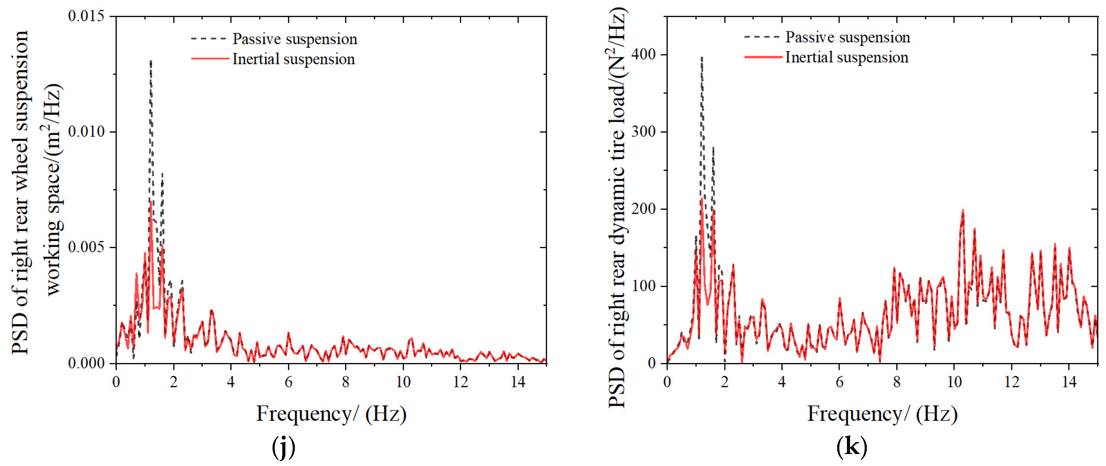
5.2. Frequency Performance Analysis

In order to analyze the performance of the inertial suspension in the frequency domain, the time domain performance indicators diagram under random road input at 20 m/s is obtained by Fourier transform, and the power spectral density comparison diagram at 1–15 Hz is obtained, as shown in Figure 7.

As can be seen from Figure 7, compared with passive suspension, the performance of the inertial suspension based on dynamic surface control is better, especially in the low frequency band 0–3 Hz, where the peak power spectral density of the inertial suspension decreases significantly. It can be concluded that the inertial suspension based on dynamic surface control can significantly improve the vibration isolation performance of the vehicle suspension in the frequency domain and effectively improve the ride comfort of the vehicle.

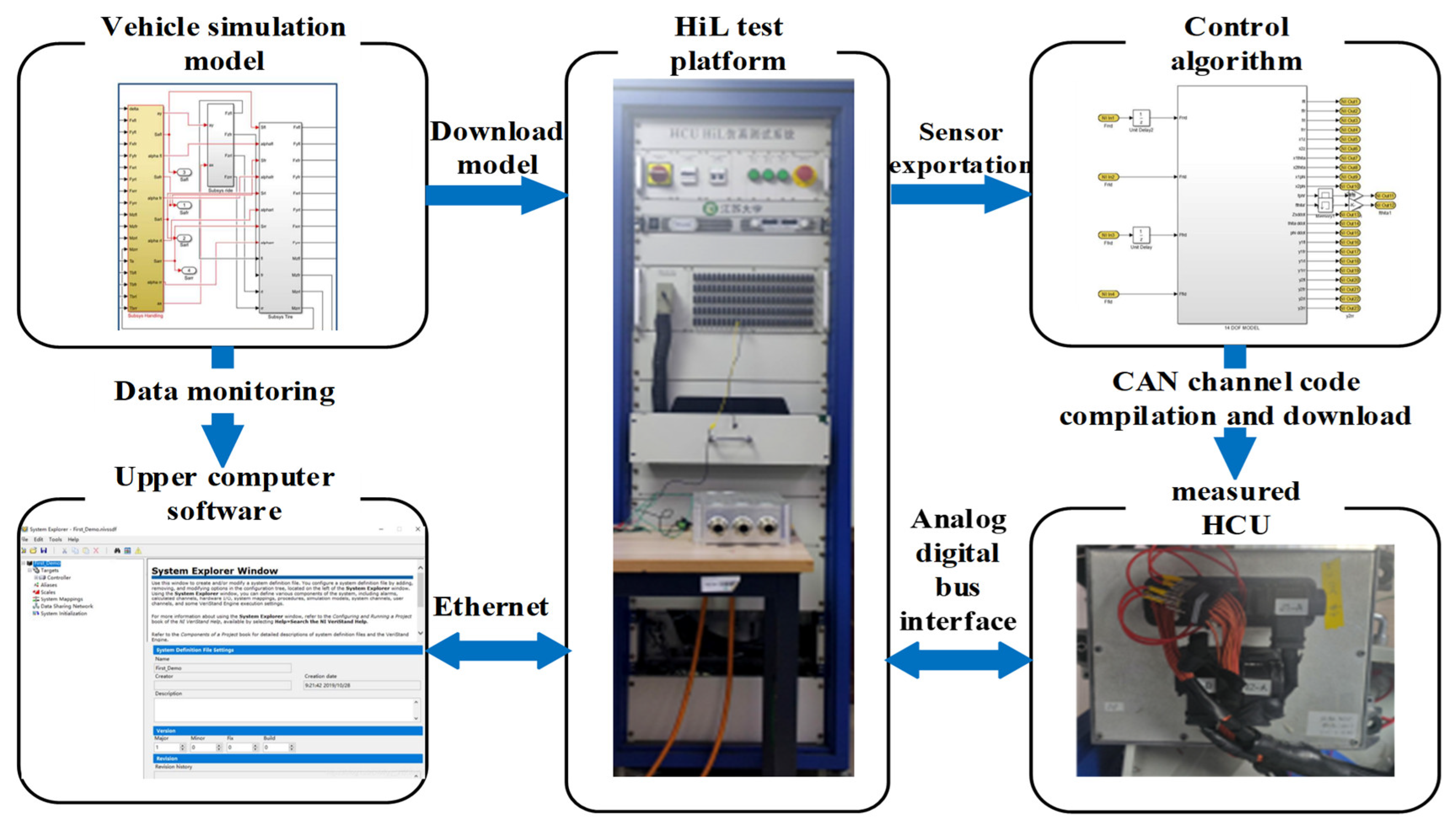
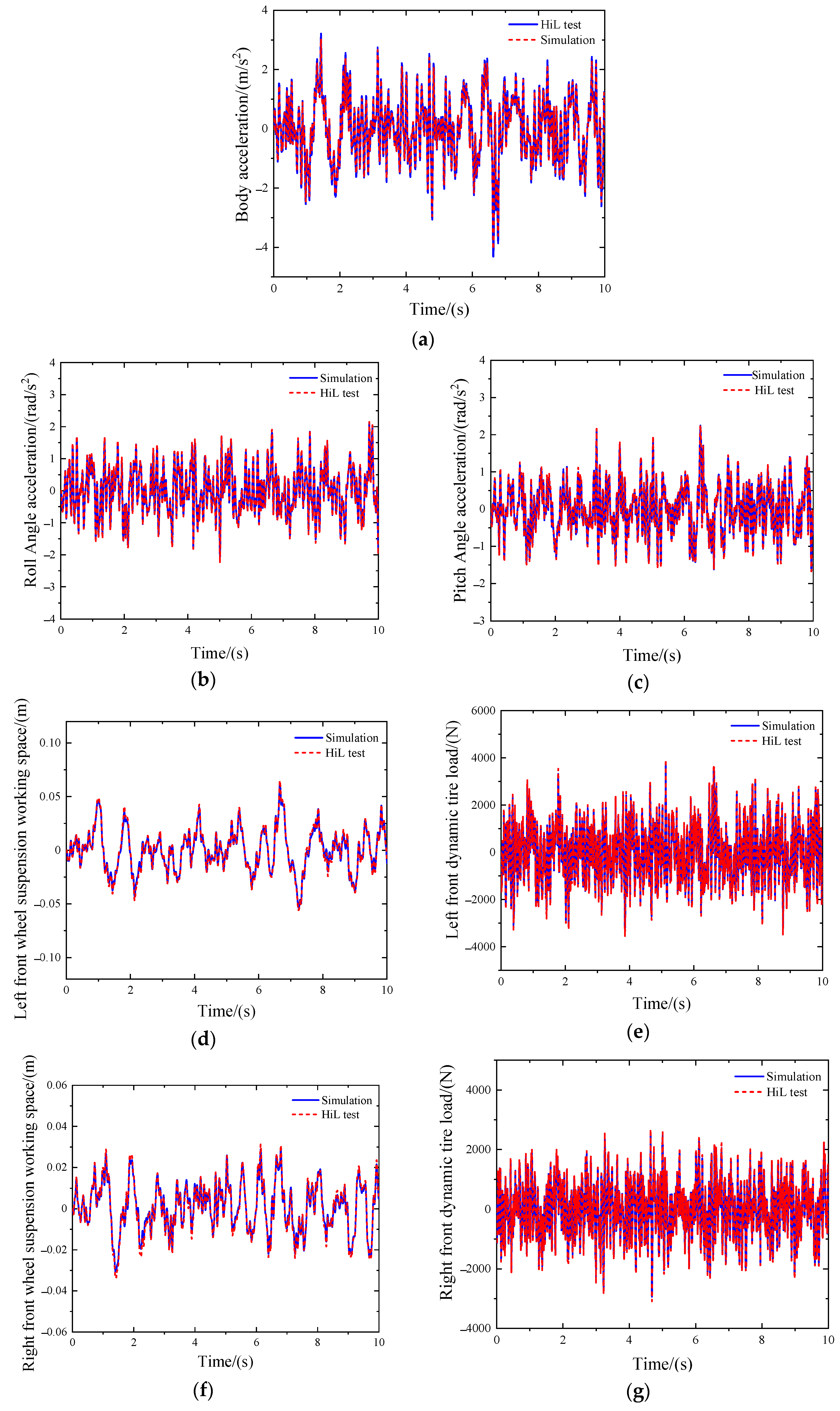
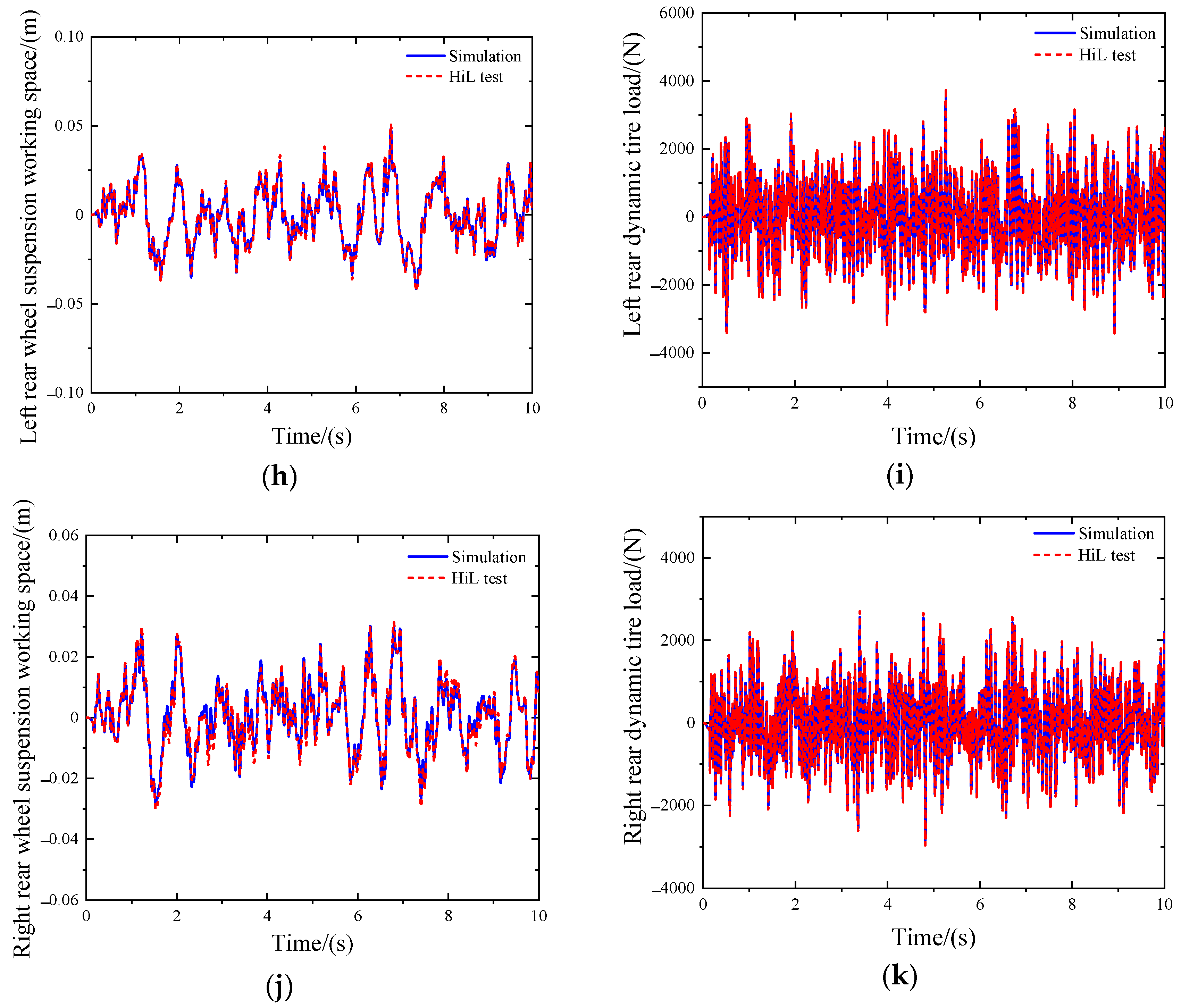
6. Verification Analysis of HiL Test

In this section, the overall layout scheme of Hybrid Control Unit (HCU) HiL test is designed, the dynamic surface control algorithm is written into the physical HCU, and the HiL test is carried out to obtain the control effect of the dynamic surface control algorithm in the physical controller HCU. The test and simulation results are compared to analyze the error size of the RMS value of its performance indicators. It is proven that the dynamic surface controller designed in this paper can run normally and reliably in the physical controller HCU.

The overall scheme of vehicle inertial suspension HiL test based on dynamic surface control is shown in Figure 8.

In order to increase the persuasiveness of the inertial suspension control algorithm based on dynamic surface control and make it run in the real vehicle controller, the test condition is set to run in a straight line under the C-class random road input of 20 m/s, so as to ensure that the test results of HiL are similar to the simulation results. Figure 8 shows the comparison of simulation results and HiL test results of performance indicators of the inertial suspension based on dynamic surface control.

Figure 9 and

Table 5. RMS and errors of HiL and simulation test performance indicators.

Performance Indicators	Simulation	HiL	Error
Body acceleration/(m·s−2)	1.0406	1.1006	5.76%
Roll angle acceleration/(rad·s−2)	0.7054	0.7401	4.91%
Pitch angle acceleration/(rad·s−2)	0.6495	0.6697	3.12%
Left front wheel suspension working space/(m)	0.0191	0.0203	6.35%
Left front dynamic tire load/(kN)	1.0999	1.1550	5.01%
Right front wheel suspension working space/(m)	0.0116	0.0124	7.42%
Right front wheel dynamic tire load/(kN)	0.8272	0.8688	5.03%
Left rear suspension working space/(m)	0.0158	0.0164	4.05%
Left rear dynamic tire load/(kN)	1.0469	1.0910	4.21%
Right rear wheel suspension working space/(m)	0.0112	0.0117	4.13%
Right rear dynamic tire load/(kN)	0.8166	0.8496	4.03%

show the time domain curves and RMS values of body acceleration, body roll angle acceleration, body pitch angle acceleration, suspension working space, and dynamic tire load of the inertial suspension based on dynamic surface control in simulation and HiL test, respectively. It can be seen from Table 5 that in the HiL test, the RMS values of the body acceleration, roll angle acceleration, and pitch angle acceleration of the inertial suspension based on dynamic surface control are 5.76%, 4.91%, and 3.12% compared with the simulation results, which are shown in Figure 9. The performance indicators of the suspension based on the HiL test are consistent with the simulation results, and the error is controlled within 8%. In summary, the experimental results show that the controller based on dynamic surface control designed in this paper can meet the needs of vehicle controllers.

7. Results

The 14-DOF vehicle suspension model was constructed, the multi-objective function for vehicle riding comfort was formulated, and the parameters were optimized through the NSGA-II algorithm. By solving the position error equations in vertical, roll, and pitch directions, and designing the intermediate dummy variable under dynamic surface control based on the Lyapunov function, the dynamic surface control law in vertical, roll, and pitch directions is obtained. Then, by solving the pseudo-inverse matrix in vertical, roll, and pitch directions, the thrust force of mechatronic inerter is obtained. Under random road input, compared with the passive suspension, the RMS value of the body acceleration, the RMS value of the body roll angle acceleration, and the RMS value of the body pitch angle acceleration of the inertial suspension based on the dynamic surface control are reduced by 23.73%, 15.28%, and 15.19%, respectively, and ride comfort of the vehicle are effectively improved.

In the simulation of the connected controller, the feasibility and practicability of the control algorithm running in the real HCU are verified. The error between the test results and the simulation results under the random road surface is about 8%.

References

1. Shuping, C.; Bin, Z. Automobile Construction; China Machine Press: Beijing, China, 2007. [Google Scholar]
2. Qin, Y.C.; Zhao, Z.; Wang, Z.F.; Li, G. Study of longitudinal–vertical dynamics for in-wheel motor-driven electric vehicles. Automot. Innov. 2021, 4, 227–237. [Google Scholar] [CrossRef]
3. Yang, X.; Zhang, T.; Shen, Y.; Liu, Y.; Bui, V.; Qiu, D. Tradeoff analysis of the energy-harvesting vehicle suspension system employing inerter element. Energy 2024, 308, 132841. [Google Scholar] [CrossRef]
4. Shen, Y.; Chen, A.; Du, F.; Yang, X.; Liu, Y.; Chen, L. Performance enhancements of semi-active vehicle air ISD suspension. Proc. Inst. Mech. Eng. Part D-J. Automob. Eng. 2024. [Google Scholar] [CrossRef]
5. Zhao, D.; Yin, Y.; Ni, T.; Zhang, W. Research review on chassis integrated control of heavy duty truck. J. Yanshan Univ. 2020, 44, 189–197. [Google Scholar]
6. Pan, G.; Ding, C.; Wang, W.; Li, A. Application of extended zero moment point in vehicle pitch control evaluation and Active control. J. Jiangsu Univ. (Nat. Sci. Ed.) 2021, 42, 85–91. [Google Scholar]
7. Jiang, Z.; Zheng, M.; Zhang, N. Research on pitch dynamics of semi-active anti-pitch hydraulic interconnected suspension. J. Vib. Shock 2020, 39, 272–278. [Google Scholar]
8. Xia, P. Simulation study on effect of multi-axle vehicle suspension system on roll stability. Master’s Thesis, Wuhan University of Technology: Wuhan, China, 2015. [Google Scholar]
9. Anafjeh, B.; Moosavi, H.; Danesh, M. Active optimal roll control of railway vehicles in curved tracks using an electrically actuated anti-roll bar System. Int. J. Control. Autom. Syst. 2023, 21, 1127–1142. [Google Scholar] [CrossRef]
10. Jiang, H.; Wang, Y.; Wu, Y.; Wang, P. Cooperative control strategy for lateral stability and roll prevention of four-wheel drive electric vehicle. J. Jilin Univ. (Eng. Technol. Ed.) 2024, 54, 540–549. [Google Scholar]
11. Li, Y.; Chi, Y.; Ji, X.; Liu, Y.; Wu, J. Research on path tracking and anti-roll cooperative control of commercial vehicle based on pareto optimal equilibrium theory. Automot. Eng. 2019, 41, 654–661+687. [Google Scholar]
12. Zhang, L.; Zhou, J.; Cheng, Q.; Wu, G. Estimation and active control of vehicle roll state considering road uneven input. J. Vib. Shock. 2018, 37, 133–141+154. [Google Scholar]
13. Pan, G.; Ding, C.; Li, Y. Research on vehicle roll evaluation index and roll control based on zero moment point. Chin. J. Mech. Eng. 2023, 59, 175–187. [Google Scholar]
14. Li, S.; Du, P.; Feng, X. Integrated control strategy of anti-rollover chassis for minibus. J. Jiangsu Univ. (Nat. Sci. Ed.) 2022, 43, 131–138. [Google Scholar]
15. Zhao, S.; Li, Y.; Yu, Q. Vehicle stability control based on coordinated control of chassis sub-systems. J. Traffic Transp. Eng. 2015, 15, 77–85. [Google Scholar]
16. Chen, G.; Lv, S.; Li, G.; Dai, J.; Yang, Z. Research on semi-vehicle semi-active fuzzy PI control suspension based on particle swarm optimization. J. Henan Univ. Technol. (Nat. Sci. Ed.) 2020, 39, 69–79. [Google Scholar]
17. Chen, G.; Xu, X.; Tang, Y.; Jiang, G. A Three-Axis Unmanned Vehicle Hydraulic Drive System and Its Comprehensive Energy-Saving Control. Strategy. Patent 202211532845.6, 18 April 2023. [Google Scholar]
18. Liang, J.; Lu, Y.; Pi, D.; Yin, G.; Zhuang, W.; Wang, F.; Feng, J.; Zhou, C. A decentralized cooperative control framework for active steering and active suspension: Multi-agent approach. IEEE Trans. Transp. Electrif. 2021, 8, 1414–1429. [Google Scholar] [CrossRef]
19. Shen, Y.; Jia, M.; Yang, X.; Liu, Y.; Chen, L. Vibration suppression using a mechatronic PDD-ISD-combined vehicle suspension system. Int. J. Mech. Sci. 2023, 250, 108277. [Google Scholar] [CrossRef]
20. Škrjanc, I. A decomposed-model predictive functional control approach to air-vehicle pitch-angle control. J. Intell. Robot. Syst. Theory Appl. 2007, 48, 115–127. [Google Scholar] [CrossRef]
21. Margolis, D.L. Semi-active heave and pitch control for ground vehicles. Veh. Syst. Dyn. 1982, 11, 31–42. [Google Scholar] [CrossRef]
22. Cao, J.T.; Liu, H.H.; Li, P.; Brown, D.J.; Dimirovski, G. A study of electric vehicle suspension control system based on an improved half-vehicle model. Int. J. Autom. Comput. 2007, 4, 236–242. [Google Scholar] [CrossRef]
23. Poussot, V.C.; Sename, O.; Dugard, L.; Gáspár, P.; Szabó, Z.; Bokor, J. A new semi-active suspension control strategy through LPV technique. Control. Eng. Pract. 2008, 16, 1519–1534. [Google Scholar] [CrossRef]
24. De, F.P.; Tanelli, M.; Corno, M.; Savaresi, S.M.; Santucci, M.D. Electronic stability control for powered two-wheelers. IEEE Trans. Control. Syst. Technol. 2014, 22, 265–272. [Google Scholar]
25. Liu, Y.; Shi, D.; Du, F.; Yang, X.; Zhu, K. Topological optimization of vehicle ISD suspension under steering braking condition. World Electr. Veh. J. 2023, 14, 297. [Google Scholar] [CrossRef]
26. Zhang, Y.; Zhang, J. Numerical simulation of stochastic road process using white noise filtration. Mech. Syst. Signal Process. 2005, 20, 363–372. [Google Scholar]
Figure 1. Vehicle control model.
Actuators 13 00389 g001
Figure 2. Structure of vehicle inertial suspension.
Actuators 13 00389 g002
Figure 3. Pavement excitation displacement of the left front wheel and the right front wheel.
Actuators 13 00389 g003
Figure 4. Flowchart of the NSGA-II algorithm.
Actuators 13 00389 g004
Figure 5. Schematic diagram of dynamic surface control system of inertial suspension based on hydraulic and electric coupling inerter.
Actuators 13 00389 g005
Figure 6. Comparison of performance response of inertial suspension. (a) Body acceleration. (b) Roll angle acceleration. (c) Pitch angle acceleration. (d) Left front wheel suspension working space. (e) Left front dynamic tire load. (f) Right front wheel suspension working space. (g) Right front dynamic tire load. (h) Left rear wheel suspension working space. (i) Left rear dynamic tire load. (j) Right rear wheel suspension working space. (k) Right rear dynamic tire load.
Actuators 13 00389 g006aActuators 13 00389 g006bActuators 13 00389 g006c
Figure 7. Power spectral density analysis of inertial suspension performance parameters. (a) Body acceleration. (b) Roll angle acceleration. (c) Pitch angle acceleration. (d) Left front wheel suspension working space. (e) Left front dynamic tire load. (f) Right front wheel suspension working space. (g) Right front dynamic tire load. (h) Left rear wheel suspension working space. (i) Left rear dynamic tire load. (j) Right rear wheel suspension working space. (k) Right rear dynamic tire load.
Actuators 13 00389 g007aActuators 13 00389 g007bActuators 13 00389 g007c
Figure 8. Design of HiL test scheme of vehicle inertial suspension based on dynamic surface control theory.
Actuators 13 00389 g008
Figure 9. HiL and simulation test results. (a) Body acceleration. (b) Roll angle acceleration. (c) Pitch angle acceleration. (d) Left front wheel suspension working space. (e) Left front dynamic tire load. (f) Right front wheel suspension working space. (g) Right front dynamic tire load. (h) Left rear wheel suspension working space. (i) Left rear dynamic tire load. (j) Right rear wheel suspension working space. (k) Right rear dynamic tire load.
Actuators 13 00389 g009aActuators 13 00389 g009b